Axionic dark matter signatures in various halo models
Abstract
In the present work we study possible time signatures Axion Dark Matter searches employing resonant cavities for various halo models. We study in particular the time dependence of the resonance width (modulation) and possible asymmetries in directional experiments.
1 Introduction
The axion has been proposed a long time ago as a solution to the strong CP problem [1] resulting to a pseudo Goldstone Boson [2, 3, 4, 5, 6], but it has also been recognized as a prominent dark matter candidate [7]. In fact, realizing an idea proposed a long time ago by Sikivie [8], various experiments such as ADMX and ADMX-HF collaborations [9, 10], [11],[12] are now planned to search for them. In addition, the newly established center for axion and physics research (CAPP) has started an ambitious axion dark matter research program [13], using SQUID and HFET technologies [14]. The allowed parameter space [15], containing information for all the axion like particles, defines a region for invisible axions, which can be dark matter candidates.
In the present work we will assume that the axion is non relativistic with mass in eV-meV scale, moving with an average velocity which is c. It is expected to be observed in resonance cavities with a width that depends on the axion mean square velocity in the local frame. The latter depends on the assumed halo model. We will expand and improve our previous work [16, 17] by including various popular halo models. We will study the time variation of the width due to the motion of the Earth around the sun and possible asymmetries with regard to the sun’s direction of motion as it goes around the center of the galaxy. Due to the rotation of the Earth around its axis these asymmetries in the width of the resonance will manifest themselves in their diurnal variation. These important signatures may become more needed, if indeed the predicted axion to photon coupling becomes weaker as some recent models predict [18].
2 Brief summary of the formalism
The photon axion interaction is dictated by the Lagrangian:
| (2.1) |
where and are the electric and magnetic fields, a model dependent constant of order one
[9],[19][20] and the axion decay constant. Axion dark matter detectors [19] employ an external magnetic field, in the previous equation, in which case one of the photons is replaced by a virtual photon, while the other maintains the energy of the axion, which is its mass plus a small fraction of kinetic energy.
The power produced, see e.g. [9], is given by:
| (2.2) |
is the loaded quality factor of the cavity. Here we have assumed is smaller than the axion width , see below. More generally, should be substituted by min (, ). This power depends on the axion density and is pretty much independent of the velocity distribution.
The axion power spectrum, which is of great interest to experiments, is written as a Breit-Wigner shape [19], [21]:
| (2.3) |
Since in the axion DM search case the cavity detectors have reached such a very high energy resolution [22, 23], one should try to accurately evaluate the width of the expected power spectra in various theoretical models.
3 Evaluation of the width in the local frame
We will derive the expression for the width assuming in the galactic frame a Maxwell Boltzmann axion velocity distribution:
| (3.4) |
We will use the relation
| (3.5) |
or
In the galactic frame the number of axions in the with frequency between and in a solid angle is
| (3.6) |
Introducing the variable we find:
| (3.7) |
The maximum of the distribution occurs at . The width at half maximum is with the roots of the equation
We thus find . Thus the width at half maximum in frequency space is:
| (3.8) |
where the last quantity is the average of the square of the axion velocity in the galactic frame.
Our next task is to transform the velocity distribution from the galactic to the local frame. The needed equation, see e.g. [24], is:
| (3.9) |
with , a unit vector in the Sun’s direction of motion, a unit vector radially out of the galaxy in our position and . The last term in the first expression of Eq. (3.9) corresponds to the motion of the Earth around the Sun with being the ratio of the modulus of the Earth’s velocity around the Sun divided by the Sun’s velocity around the center of the Galaxy, i.e. km/s and . The above formula assumes that the motion of both the Sun around the Galaxy and of the Earth around the Sun are uniformly circular. The exact orbits are, of course, more complicated but such deviations are not expected to significantly modify our results. In Eq. (3.9) is the phase of the Earth ( around the beginning of June)#1#1 #1 One could, of course, make the time dependence of the rates due to the motion of the Earth more explicit by writing , where is the fraction of the year..
In the local frame , ignoring the motion of the Earth, we make in the velocity distribution the substitution:
where is the speed of the sun around the center of the galaxy and , is a unit vector in the sun’s direction of motion. Thus Eq. (3.7)
| (3.10) |
The function is exhibited in Fig. 3.1.


has extrema at
The first of these yields a maximum for all , while the second is the location of a maximum only for .
Clearly the width at half maximum is a function of . Its value is obtained numerically and it is exhibited in Fig. 3.2a,b, corresponding to whether the sense of direction of the axion can be determined or not. The width clearly has a maximum opposite to the sun’s direction of motion (a), if the sense of direction of the axion can be determined, something perhaps not very realistic. It exhibits simply a minimum in the plane perpendicular to the sun’s velocity, in the most realistic scenario that the sense of direction cannot be determined (b).


radians
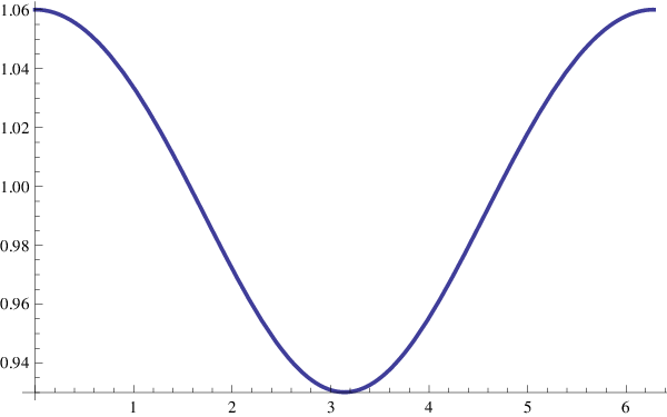
We will next consider the effect of the Earth’s motion in the standard, non directional, experiments. The azymouthal angle () dependence, averages out to zero. Thus the distribution takes the form:
| (3.11) |
The maximum of the distribution occurs at the root of the equation :
which is obtained graphically. Then where and are the roots of the equation:
where
The obtained results are exhibited in Fig. 3.3.
radians
4 More complicated velocity distributions
In the context of dark matter other velocity distributions have been considered, e.g. completely phase-mixed DM, dubbed “debris flow” (Kuhlen et al. [25]) and caustic rings (Sikivie [26],[27][28], Vergados [29].
4.1 The case of debris flows
In the case of debris flows one assumes a dark matter distribution which is of the form:
| (4.12) |
with
| (4.13) |
where
| (4.14) |

The introduction of debris flows has two effects:
- 1.
It shifts the maximum of the distribution, without changing the location of the maximum .
(4.15) with
(4.16) - 2.
The width at half maximum is affected:
(4.17)


We thus find:
- 1.
In the galactic frame:
respectively
- 2.
In the local frame:
respectively
The modulation of the width is exhibited in Fig. 4.6.
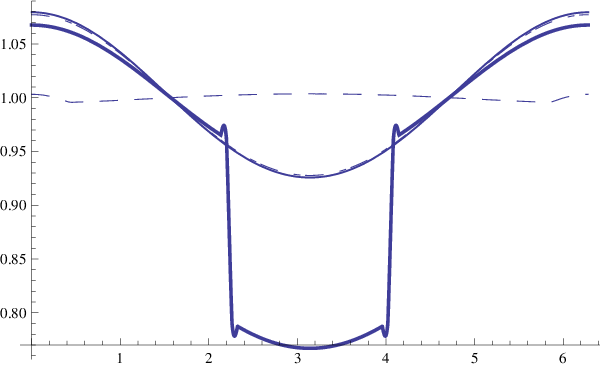
The width expected in directional experiments is shown in Fig. 4.7.


4.2 The case of caustic rings
Our study of the phase space structure of the Milky Way halo is motivated in large part by the ongoing searches for dark matter on Earth, using axion, see e.g. [14, 11], and WIMP detectors, see e.g. [30, 31, 32, 33, 34]. The signal in such detectors depends on the velocity distribution of dark matter in the solar neighborhood. The caustic ring halo model predicts , see e.g. [28], that most of the local dark matter is in discrete flows and provides the velocity vectors and densities of the first forty flows at the Earth’s location in the Galaxy, which are essential when interpreting a signal in a dark matter detector on Earth. In principle the halo model can be treated as phase-mixed DM leading to a linear combination of a M-B distribution and one appropriate to caustic rings, in a fashion similar to that with debris flow discussed above. We will, however, concentrate here in caustic rings.
The relevant information for our purposes can be extracted from table V of Duffy and Sikivie [28], which has improved and updated earlier versions, and for the reader’s convenience is summarized in table 4.1. One then writes the velocity distribution as
| (4.18) |
where are the components of the velocity components in our notation. are suitable normalization factors extracted from the corresponding densities of the last columns of table 4.1.
| km/s | km/s | km/s | km/s | |||
|---|---|---|---|---|---|---|
With these ingredients we compute the modulated widths, see Fig. 4.8. We observe that the difference between the maximum and the minimum is . Note, however, that the maximum is shifted from (June third) , i.e. to approximately two weeks later. This is expected due to the asymmetries in the caustic velocity distribution. We also have obtained the directional dependence of the width, see Fig. 4.9. We note, however, that in this case the width depends on the azymouthal angle . This does not occur in the case of symmetric velocity distributions so long as the velocity of the Earth is neglected. Here the variation can be sizable for directions of observation lying in a plane perpendicular to the sun’s velocity, but small away from it. This is another special signature of the caustic ring scenario. Anyway in this case one need not know the sense of direction of the axion.


. The effect is now small.
5 Discussion
In the present work we discussed the time variation of the width of of the axion to photon resonance cavities involved in Axion Dark Matter Searches, by considering a number of popular halo models. We find two important signatures:
- 1.
Annual variation due to the motion of the Earth around the sun. We find that in the relative width, i.e. the width divided by its time average, can attain significant differences between the maximum expected in June and the minimum expected six months later. This variation is larger than the modulation expected in ordinary dark matter of WIMPs. It does not depend on the geometry of the cavity or other details of the apparatus. It depends somewhat on the assumed velocity distribution.
- 2.
The width depends strongly of the angle of direction of observation relative to the sun’s direction of motion, even if the sense of direction is not known. This can manifest itself as a characteristic diurnal variation due to the rotation of the Earth around its own axis (see our earlier work [16] on how one can translate the directional data into diurnal variation). Anyway once such a device is operating, data can be taken as usual. Only one has to bin them according the time they were obtained. If a potentially useful signal is found, a complete analysis can be done according the directionality to firmly establish that the signal is due to the axion.
In conclusion in this work we have elaborated on two signatures that might aid the analysis of axion dark matter searches. Eventually, if such an observation is made, one may be able to exploit the results obtained here to gain information about the velocity distribution associated with the various halo models.
References
- [1] R. Peccei, H. Quinn, Phys. Rev. Lett 38 (1977) 1440.
- [2] S. Weinberg, Phys. Rev. Lett. 40 (1978) 223.
- [3] F. Wilczek, Phys. Rev. Lett. 40 (1978) 279.
- [4] J. Preskill, M. B. Wise, F. Wilczek, Phys. Lett. B120 (1983) 127.
- [5] L. F. Abbott, P. Sikivie, Phys. Lett. B120 (1983) 133.
- [6] M. Dine, W. Fischler, Phys. Lett. B120 (1983) 137.
- [7] J. Primack, D. Seckel, B. Sadoulet, Ann. Rev. Nuc. Par. Sc. 38 (1988) 751.
- [8] P. Sikivie, Phys. Rev. Lett. 51 (1983) 1415.
- [9] I. P. Stern, ArXiv 1403.5332 (2014) physics.ins–det, on behalf of ADMX and ADMX-HF collaborations, Axion Dark Matter Searches.
- [10] G. Rybka, The Axion Dark Matter Experiment, IBS MultiDark Joint Focus Program WIMPs and Axions, Daejeon, S. Korea October 2014.
- [11] S. J. Asztalos, et al., Phys. Rev. Lett. 104 (2010) 041301, the ADMX Collaboration, arXiv:0910.5914 (astro-ph.CO).
- [12] A. Wagner, et al., Phys. Rev. Lett. 105 (2010) 171801, for the ADMX collaboration; arXiv:1007.3766 (astro-ph.CO).
- [13] Center for Axion and Precision Physics research (CAPP), Daejeon 305-701, Republic of Korea. More information is available at http:.
- [14] S. J. Asztalos, et al., Nucl. Instr. Meth. in Phys. Res. A656 (2011) 39, arXiv:1105.4203 (physics.ins-det).
- [15] G. Raffelt, Astrophysical Axion Bounds , IBS MultiDark Joint Focus Program WIMPs and Axions, Daejeon, S. Korea October 2014.
- [16] Y.Semertzidis, J.D.Vergados, Nuc. Phys. B 897 (2015) 821, arXiv:1412.6907 (hep-ph).
- [17] Y. Semertzidis and J. D. Vergados, Proceedings of the 18th International Conference: From the Planck Scale to the Electroweak Scale 25-29 May 2015 Ioannina, Greece, arXiv:1511.08516 (astro-ph.GA).
- [18] Y. H. Ahn, Flavored Peccei-Quinn symetry, arXiv:1410.1634 [hep-pj].
- [19] J. Hong, J. E. Kim, S. Nam, Y. Semertzidis, arXiv:1403.1576 (2014) physics.ins–det, calculations of Resonance enhancement factor in axion-search tube experiments.
- [20] J. E. Kim, Phys. Rev. D 58 (1998) 055006.
- [21] L. Krauss, J. Moody, F. Wilczek, D. Morris, Phys. Rev. Lett. 55 (1985) 1797.
- [22] L. Duffy, et al., Phys. Rev. Lett. 95 (2005) 09134, for the ADMX Collaboration.
- [23] L. Duffy, et al., Phys. Rev. D 74 (2006) 012006, for the ADMX Collaboration.
- [24] J. Vergados, Phys. Rev. D. 85 (2012) 123502, ; arXiv:1202.3105 (hep-ph).
- [25] M. Kuhlen, M. Lisanti, D. Speregel, Phys. Rev. D 86 (2012) 063505, arXiv:1202.0007 (astro-ph.GA).
- [26] P. Sikivie, Phys. Rev. D 60 (1999) 063501.
- [27] P. Sikivie, Phys. Lett. B 432 (1998) 139.
- [28] L. D. Duffy, P. Sivie, Phys. Rev. D 78 (2008) 063508.
- [29] J. D. Vergados, Phys. Rev. D 63 (2001) 063511.
- [30] E. Aprile, et al., Phys. Rev. Lett. 107 (2011) 131302, arXiv:1104.2549v3 [astro-ph.CO].
- [31] R. Bernabei, et al., Int. J. Mod. Phys A 28 (2013) 1330022, dOI: 10.1142/S0217751X13300226.
- [32] E. Armengaud, et al., Phys. Lett. B 702 (2011) 329, arXiv:1103.4070v3 [astro-ph.CO].
- [33] D. Akerib, et al., Phys. Rev. Lett. 96 (2006) 011302, arXiv:astro-ph/0509259 and arXiv:astro-ph/0509269.
- [34] K. Abe, et al., Astropart. Phys. 31 (2009) 290, arXiv:v3 [physics.ins-det]0809.4413v3 [physics.ins-det].