Gauss-Bonnet for multi-linear valuations
Abstract.
We prove Gauss-Bonnet and Poincaré-Hopf formulas for multi-linear valuations on finite simple graphs and answer affirmatively a conjecture of Grünbaum from 1970 by constructing higher order Dehn-Sommerville valuations which vanish for all -graphs without boundary. A first example of a higher degree valuations was introduced by Wu in 1959. It is the Wu characteristic with which sums over all ordered intersecting pairs of complete subgraphs of a finite simple graph . It more generally defines an intersection number , where are the simplices in two subgraphs of a given graph. The self intersection number is a higher order Euler characteristic. The later is the linear valuation which sums over all complete subgraphs of . We prove that all these characteristics share the multiplicative property of Euler characteristic: for any pair of finite simple graphs, we have so that all Wu characteristics like Euler characteristic are multiplicative on the Stanley-Reisner ring. The Wu characteristics are invariant under Barycentric refinements and are so combinatorial invariants in the terminology of Bott. By constructing a curvature satisfying Gauss-Bonnet , where runs over all vertices we prove which holds for any -graph with boundary . There also prove higher order Poincaré-Hopf formulas: similarly as for Euler characteristic and a scalar function , where the index with satisfies , there is for every multi-linear valuation and function an index such that . For -graphs and it agrees with the Euler curvature. For the vanishing multi-valuations which were conjectured to exist, like for the quadratic valuation with on -graphs, discrete 4 manifolds, where is the -matrix counting the number of -simplices in intersecting with -simplices in , the curvature is constant zero. For general graphs and higher multi-linear Dehn-Sommerville relations, the Dehn-Sommerville curvature at a vertex is a Dehn-Sommerville valuation on the unit sphere . We show for any linear valuation of a -graph with -vector . This leads to multi-linear Dehn-Sommerville valuations which vanish on -graphs.
Key words and phrases:
Graph theory, Euler characteristic, Wu characteristic, Valuations, Barycentric characteristics, Discrete Intersection Theory1991 Mathematics Subject Classification
53A55, 05C99, 52C99, 57M15, 68R99, 53C651. Introduction
Given a finite simple graph , a valuation is a real-valued map on the set of
subgraphs of , so that holds for any two subgraphs
of and . Here and ,
if are finite simple graphs with vertex sets and edge sets .
With the empty graph , a graph with no vertices and no edges, the set of all subgraphs is a lattice.
If one requires additionally that holds for any two isomorphic subgraphs of ,
then is called an invariant valuation.
A quadratic valuation is a map which attaches to a pair
of subgraphs of a real number such that for fixed ,
the map and for fixed
the map are valuations and such that if .
It is an intersection number which extends to a bilinear
form on the module of chains defined on the abstract Whitney simplicial complex of the graph .
More generally, a -linear valuation is a map which attaches to an ordered -tuple
of subgraphs of a real intersection number which is “multi-linear” in the sense that
any of the maps is a valuation. We also assume they are localized
in the sense that is only possible only if .
For a -linear valuation one obtains
the self intersection number . We will see that some multi-linear valuations still
honor the product property , where is the product graph,
the incidence graph of the product of the representations of in the Stanley-Reisner ring.
When seen as integer-valued functions on this ring, valuations with this property are multiplicative functions.
Here are footnotes on the choice of the definitions.
(i) The terminology “linear valuation” and “multi-linear valuation”
come from fact that the valuation property can be written as
using the symmetric difference .
But this addition throws us out of the category of graphs
into the class of chains. Valuations are in this larger ambient class compatible with the algebra.
For graphs, we have to to stick to the lattice description when defining the
valuation. An example: with the given definitions of union and intersection of graphs,
the graphs and
define and .
The valuation property is satisfied, but with symmetric differences on vertices
and edges we get which is only a chain and no more a graph.
The absence of a linear algebra structure on the category of graphs is a reason for the complexity for
computing valuations (it is an NP complete problem) and the reason to stick with the
Boolean distributive lattice of subgraphs using union and intersection rather than
symmetric difference and intersection which is not defined in the category of graphs. The usual
graph complement is not compatible. Also in the continuum, valuations use the lattice structure
using that unions and intersections of convex sets rather than allowing
complements of convex sets which would allow to build a measure theory for valuations.
In the discrete, the difficulty is transparent: for a valuation, the complement of the graph
within is only a chain which we call
the virtual interior. It has the Euler characteristic , which is the Wu characteristic of .
(ii) Without the assumption ,
we would also count constant functions as valuation, but it is tradition not to
include them. It would render the valuation “affine” rather than “linear” because linearity
requires for the empty graph .
(iii) The invariance property is also a common assumption, both in the continuum and in the discrete.
In the continuum case, where valuations are mainly studied on unions
of convex sets in Euclidean space, the invariance assumption is that the valuation is invariant under Euclidean
motion. The reason for assuming this is that the theory is already rich enough with that assumption and
that it also also in the continuum leads to a finite dimensional space of valuations. Flat Euclidean space
seems confining. This is however not the case as one can for the purpose of Valuations, embed Riemannian
manifolds into Euclidean or projective spaces. This induces a valuation theory on Riemannian manifolds and
beyond. More about this in the Hadwiger appendix.
(iv) The assumption if
was done so that the theorems work. Without it, much would fail. The assumption
excludes cases like for two linear valuations .
The assumption will imply that the curvatures and indices are localized as is the
case in differential geometry. One could look at cubic valuations for
which is only zero if the nerve graph defined by is not connected. Widening the localization
as such would make the curvature functions depend on a disk of radius , if is
a -linear valuation. With the assumption, the curvature functions always depend on a disk of radius .
The assumption of insisting all simplices to intersect simultaneously (as Wu did)
implies that cubic and higher order characteristics agree with Euler characteristic. Otherwise, the boundary
formula as well as the product property fails. We would also expect that getting rid of the localization
assumption would lead to additional “connection terms” due to chains which are not boundaries.

An example of a non-invariant valuation is the map which assigns to a sub graph of the vertex degree of a fixed vertex within . When summing this valuations over all vertices , we get by the Euler handshake formula the invariant valuation , counting twice the number of edges in . The Euler handshake is already a Gauss-Bonnet formula adding up local quantities to get a global quantity. We see it now as adding up local valuations to a global valuation. The prototype of an invariant valuation is the Euler characteristic of a graph . It is
where runs over all complete subgraphs of of non-negative dimension. It is an alternating
sum of the components of the -vector of . Each is of course an invariant valuation.
By Gauss-Bonnet, the Euler characteristic can be written as a sum of generalized local valuations or curvatures
,
where counts the number of -simplices in the unit sphere of centered at including
counting the empty graph as a dimensional simplex. The map is the curvature
of at . It is generalized as it assigns to the empty graph
the constant . Any invariant valuation can be written as a sum of such local valuations using the curvature
. This is Gauss-Bonnet for
valuations. We rediscovered it in [83] in the case of Euler characteristic but the
formula has been discovered and rediscovered before [109, 70, 50].
It appears that we have entered new ground when extending Gauss-Bonnet
to general linear valuations and especially to multi-linear valuations. It is important to note that
Gauss-Bonnet holds for all finite simple graphs and any multi-linear valuation and no geometric assumptions
whatsoever like being a discretization of a manifold are needed. The theorem holds for all networks.
An example of a quadratic valuation is the Wu characteristic [149] given by
where runs over all ordered pairs of complete subgraphs of . It can be written as a quadratic form for the -quadratic form or simply -matrix counting the number of pairs of -simplices intersecting with -simplices in :
It more generally produces an intersection number
where runs over all complete subgraphs of the subgraph and runs over
all complete subgraphs of the subgraph . In the second equivalent formula for ,
the quadratic form counts the number of -simplices in and -simplices in
with . Let be a one point graph for example,
then is a
linear valuation, but not an invariant valuation as it is local giving nonzero values
only near the vertex .
While the Euler characteristic defines a linear map on the -vector with counting the number of complete subgraphs of , the Wu characteristic evaluates a quadratic -form , where counts the number of complete subgraphs of which intersect in a non-empty graph. If we write then
and , where counts the number of intersections of -simplices in with -simplices in . The quadratic form is not necessarily positive definite but always has a positive maximal eigenvalue by Perron-Frobenius. One can also look at cubic situations like
where the behavior on complete graphs is again for all and holds for all -graphs even if has a boundary. It can be written using a cubic -form counting the number of or -simplices in which simultaneously intersect: with ,
The higher order Wu characteristics are defined similarly using -linear -forms
or -tensors. We have and .
All these characteristics turn out to be invariant under Barycentric refinement as well as have the multiplicative
property and agree up to a sign with Euler characteristic for -graphs, graphs for which every
unit sphere is a -sphere.
Euler proved with for planar graphs, where counts
not only triangles but any region defined by an embedding of into a 2-sphere.
In our terminology, graphs like the dodecahedron or cube graph are -dimensional,
as they have no triangles. Among the five Platonic solids, only the octahedron and icosahedron are
as 2-spheres, the tetrahedron is a 3-dimensional simplex, has Euler characteristic and is contractible.
We can reformulate Euler’s result then that for a discrete 2-sphere , the Euler characteristic is .
We know that is a homotopy invariant,
that it is the first Dehn-Sommerville invariant [81] and also that it is a Barycentric characteristic
number to the eigenvalue , obtained by looking at the linear map on -vector of the graph and taking an
eigenvector of and defining .
As is the number of even-dimensional simplices minus the number of odd-dimensional simplices,
it is the super trace of the identity operator on the -dimensional Hilbert space of
discrete differential forms.
It is robust under heat deformation: if is the exterior derivative, the discrete McKean-Singer formula
[113, 88] tells that
, where is the Hodge Laplacian on discrete differential forms
and if is the part of acting on -forms.
By the way, the total dimension of all discrete differential forms is an example of an
invariant valuation. It is believed that for -graphs it is bounded below by by a conjecture of
Kalai of 1989 [143] (formulated for polytopes) as one can learn in [14].
This number is also interesting as it is hard to compute for general graphs, that it is the number of vertices
of the Barycentric refinement of or the value if is the Stanley-Reisner polynomial
of . The smallest -sphere is believed to be the sharp lower bound like
attained for the graph, attained for the octahedron, for the 3-cross polytop or for the 4-cross polytop;
the reason is that for the smallest -sphere. As the Kalai valuation has the curvature
which is always positive, one could try to use Gauss-Bonnet and induction,
as implying . But since the number of
vertices of is only we have . If
one could verify the conjecture for all graphs with vertices, then the induction assumption
would give . The Kalai conjecture is already by definition verifiable in finitely
many cases for each (in principle) but the just given argument reduces the verification range from to .
The argument still gives inductively for any so that
holds for any graph with clique number . But since
for we have and if is a subgraph of ,
holds already trivially. We believe it should be possible to use Dehn-Sommerville relations to estimate
the Kalai curvature better on this space. But this requires to understand quantitatively the projection onto the
Dehn-Sommerville space and then the vector .
Due to its multi-linear nature, one can not expect much from the Wu characteristic at first. Actually, it starts with bad news: is not a homotopy invariant, as but , despite that and are homotopic. Interestingly, the Wu characteristic picks up the dimension of a simplex and so that one can write more elegantly
Note that as the case shows where , but . As is invariant under Barycentric refinement, it has been called combinatorial invariant (see section 1.2 of [20]), where polynomial functionals and were defined, which sum over all possible subsets of and where is the ’th Betti number of the graph generated by the set . Like Euler characteristics, also the Wu characteristic is a functional on the class of simplicial sub-complexes of but is not a valuation: the kite graph has but two triangular subgraphs with but so that but and . The Wu characteristic is a quadratic valuation as defined above. Just having mentioned polynomial invariants, one could combine all Wu characteristics and define the Wu function
where is the Euler characteristic, the Wu characteristic,
the cubic Wu characteristic etc. For a graph or -ball,
we have , for a -graph , the Wu function is .
The figure graph with , ,
, is already a case where we don’t yet have a closed form for .
We will see that any of the can be computed fast for most graphs as it satisfies a Poincaré-Hopf formula and for -graphs with boundary. Also etc. What happens is that the index entering in Poincaré-Hopf is a valuation on the unit sphere, allowing to apply Poincaré-Hopf again there etc. So, for most graphs in the Erdös-Renyi space of all graphs with elements, also the Wu characteristic can be computed quickly. The complexity for computing is polynomial in , if one insists for example that for any finite intersection of unit spheres, maximally 99% of all possible connections between vertices in the unit sphere are present. This especially applies for -graphs, where any finite intersection of unit spheres is a -sphere. A consequence of the boundary formula is that for 2-spheres, we still have
where . The proof of the reduction to Euler characteristic makes use of the Gauss-Bonnet result for multi-linear valuations which in particular holds for the Wu characteristics. It turns out that in the interior of a -graph, in distance 2 or larger from the boundary, the curvature of the Wu characteristic is the same than the curvature of the Euler characteristic . For odd dimensional graphs, the curvature of lives near the boundary of , similarly than the curvature for Euler characteristic. For an even dimensional graph with boundary, the curvatures for Euler characteristic or Wu characteristics are in the interior. The proof of the boundary formula reveals what needs to be satisfied: for each unit sphere, we have to be able to use induction. The formula shows that measures the Euler characteristic of a “virtual interior” of a graph. This interior is no more a graph but a chain as forming complements throws us out of the category of graphs into a larger category of chains: take the two boundary points of away, then we end up with an edge which has no vertices attached and which is not a graph any more. It is the virtual interior of and has Euler characteristic which is the Wu characteristic of . Because of invariance under Barycentric subdivision, the Wu characteristic is defined also in the continuum limit for compact manifolds with boundary , where it satisfies the same boundary formula . While expressible by Euler characteristic for discrete manifolds, the Wu invariant becomes interesting for varieties as we see already in simple examples like the lemniscate
which has the Wu characteristic
and Euler characteristic . Indeed, we can compute the curvature of the Wu-invariant at a singularity
of a projective variety by discretization using a graph. Quadratic valuations are useful too as they produce
intersection numbers for any pairs of subgraphs and so an intersection
number of a pair of varieties. Two -dimensional circular graphs
for example crossing twice have intersection number .
We restrict here to the language of graphs. This means that we look only at abstract simplicial complexes which are
Whitney complexes of some graph. Like with topologies, measure structures or other constructs placed on a set,
one could consider different simplicial complexes on the same graph.
The -dimensional skeleton-complex consisting of vertices and edges
is an example. It is too small for geometry as it treats any graph as a “curve”. The neighborhood complex is an other
example, but it renders the dimension too large; for a wheel graph with boundary for example, the
neighborhood complex would be -dimensional.. The sweet spot is the Whitney complex defined by all complete
subgraphs of . For the wheel graph for example, it renders it a discrete disc of dimension , with Euler characteristic
, which is contractible and has a -dimensional boundary . The geometry, cohomology, homotopy, even spectral
theory all behave similarly as in the continuum. The language of graphs is intuitive and
not much of generality is lost: while not every abstract finite simplicial
complex on is a Whitney complex of a finite graph - the simplicial complex with algebraic
representation is the
smallest example which fails to be a Whitney complex - the Barycentric refinement of an arbitrary
finite abstract simplicial complex is always the Whitney complex of a finite simple graph.
In the above triangle without 2-simplex, the refinement of the complex is the Whitney complex of .
Valuations on graphs satisfy a Gauss-Bonnet formula. For the valuation , this is the fundamental
theorem of graph theory, a name sometimes applied only for the Euler handshaking lemma which is Gauss-Bonnet
for . We will see that Gauss-Bonnet generalizes to multi-linear valuations but curvature depend now
on the ball of radius . The curvature remains local but
in some sense has become a second order difference operator similarly as in the continuum, where the curvature
tensor uses second derivatives. The language of graphs is equivalent but more intuitive
especially when dealing with valuations as a classically, valuation are defined as functionals on
simplicial sub complexes of a complex on so that classically; it is important to realize that a valuation
is not a map from subsets of to but a map from sets of subsets of .
It is much easier to work with real-valued maps from the set of subgraphs of to . Subgraphs have
the intuitive feel of subsets but encode simplicial complexes. The use of valuations as a functional
on the set of graphs is language which allows to work with valuations using the intuition
we know from measures.
On a graph , the discrete Hadwiger theorem [79]
assures that the dimension of the space of valuations
on is the clique number of . A basis is given by the functionals , counting the number
subgraphs of . The Euler characteristic can be characterized as
the only invariant valuation which stays the same when applying Barycentric subdivision and which assigns the value
to all simplices. The multi-linear Dehn-Sommerville invariants we are going to construct which
assign the value to -graphs are not invariant under Barycentric refinements on the class of all graphs,
but only vanish on -graphs, a class, where the Barycentric invariance is clear.
The valuation can also be characterized as the only invariant valuation which is a
homotopy invariant and which assigns to a subgraph. Similarly, an extension of the discrete Hadwiger
result of Klein-Rota shows that the space of invariant quadratic valuations
is -dimensional. A basis is given by the functionals with ,
where counts the number of pairs of -dimensional simplices and dimensional
simplices for which . For one dimensional graphs, graphs without triangles
for example, the space of linear valuations has dimension , and the space of quadratic valuations
has dimension . Graphs with maximal dimension have a vector space of linear valuations which is
two dimensional. It has a basis counting the number of vertices and edges, a spanning set for the
vector space of quadratic valuations is counting the number of vertices,
counting the number of pairs of edges intersecting and
counting the number of pairs , where is a vertex contains in an edge .
In this case, by Euler handshake but that is a relation between linear and quadratic
valuations. In an appendix, we review the discrete Hadwiger theorem and prove the extension
to quadratic valuations.
One can look at some valuations like Euler characteristic also from an algebraic point of view, as it is possible to write , where is the element in the Stanley-Reisner ring representing the graph. The later is a polynomial ring, where each vertex is represented by a variable and every monomial represents a complete subgraph. Each summand in the polynomial is a monomial. For the kite graph for example obtained by gluing two triangles and along an edge , we have and . The Z-module of chains for is the dimensional set containing elements like in which the monoids of form the basis elements. Valuations extend naturally to this module. We would for example have and and . Quadratic valuations are then quadratic forms on this module. We will write the quadratic Wu characteristic algebraically as
a representation which will together with Poincaré-Hopf imply that is multiplicative when taking Cartesian products of graphs. It reminds of variance in probability theory. Similarly,
reminds of covariance if the evaluation is
identified with “expectation”. In some sense therefore, if Euler characteristic is a topological
analog of expectation, the quadratic Wu characteristic is a topological analogue
of variance and the product formulas for two graphs an analogue of
which all hold for independent random variables as are then uncorrelated.
For general networks, there is no relation between Euler characteristic and Wu characteristic.
It fits the analogy as for general random variables where no relation between expectation and variance exists in general.
The fact that for discrete manifolds without boundary, the Euler and Wu characteristics agree,
and for discrete manifolds with boundary, the Euler and cubic Wu characteristic agree, comes
unexpectedly. We were certainly surprised when discovering this experimentally. Note however that in the
entire Erdös-Renyi space of networks with vertices, the geometric -graphs form a very thin slice.
(While both growth rates are not known, one can expect that the number of non-isomorphic -graphs with
vertices is bounded above by , an estimate coming from partitioning into connected
components, while the number of non-isomorphic graphs with
vertices should have a lower bound of the form for some positive , an estimate expected to hold as
most pairs of graphs are not isomorphic.)
The reason for the multiplicative property is partly algebraic but there is a topological twist required.
This is the Poincaré-Hopf formula which allows to make the connection from algebra to geometry:
lets look at Euler characteristic which sums up over all complete subgraphs
of the graph . Since is an integer-valued function on the vertex set of the
Barycentric refinement graph , one can ask whether it is the Poincaré-Hopf index
of a scalar function on the vertex set of . As Poincaré-Hopf tells
and , it would be nice if there existed a function for which .
When investigating this experimentally we were surprised to see that this is indeed the case.
The scalar function which enumerates the monomials of the Stanley-Reisner polynomial
defined by , where the monomials are ordered according to dimension and lexicographic order, does the job.
The proof reveals that the sub graph of generated by
is a -sphere
if the dimension of is . This implies .
This computation works for any finite simple graph and no geometric assumption on is necessary.
It shows the remarkable fact that the dimension signature on the Barycentric refinement of any
finite simple graph is actually a Poincaré-Hopf index of a gradient vector field on the graph. There is
no continuum analogue of that; only a shadow of this result can be seen in the proof of the classical
Poincaré-Hopf theorem in differential topology [139], where one proofs the theorem first
for a particular gradient vector field defined by a triangulation and then proves by a deformation
argument that the Poincaré-Hopf sum does not depend on the field.
As the Euler characteristic is the only multiplicative linear invariant valuation on the set
of graphs, we have to go beyond linear valuations to get more multiplicative invariant functionals of this type.
Quadratic valuations are the next natural choice and the Wu characteristic is a natural
quadratic valuation as it is invariant under Barycentric refinements,
assigns the same value to isomorphic subgraphs and assigns the value to the empty graph and the value
to the one point graph . Similarly, the cubic Wu characteristic is a cubic valuation with
this property. The Euler characteristic and the Wu characteristics (including cubic and higher order versions)
more generally appear to be the only multiplicative invariant valuations among all multi-linear invariant valuations.
Grünbaum objected to the claim of Wu that the Wu characteristics
are the only combinatorial invariants and pointed out the existence of Dehn-Sommerville invariants.
This is a valid objection but Wu’s hypothesis could still hold when one looks at it as a
functionals on all graphs. It is well known that the Euler characteristic is the only
invariant valuation which assigns the value to and is a combinatorial invariant
[50, 109].
The Wu characteristic appears to be the only quadratic invariant valuation on the class of all finite simple graphs
which is invariant under Barycentric refinement and assigns the value to .
If that is true, we could also say that is the only quadratic invariant valuation
which is multiplicative. However - and that is the point which Grünbaum made in the case of Euler characteristic -
is that in geometric situations like what we call -graphs, there are other valuations, the Dehn-Sommerville
invariants, which are on this class also invariant under Barycentric subdivision because they are zero, even so
the values of refinements explode in general when applying refinements in the class of general networks.
At present, we must consider it an open problem, whether the Wu invariant is the only quadratic valuation
on the class of all graphs, which is invariant under Barycentric refinements and assigns to every subgraph.
Lets call the statement of uniqueness of Wu characteristic the Wu hypothesis. To understand it, we have
to investigate the behavior of the -matrix under Barycentric refinement, something we have only just started to look
at. The fact that -vectors transform linearly and looking at the eigenvectors shows immediately that the
Euler characteristic is unique. If the transformation on -matrices were linear, we expect a unique
eigenvector to the eigenvalue . This would be the Wu eigenvector, leading to the uniqueness of Wu characteristics.
If the quadratic case works, then most likely also more general -linear valuations work and be unique
in the class of -linear valuations which are invariant under Barycentric refinement as well as assigning to
a single vertex.
In a finite simple graph , a complete subgraph is also called a face or simplex.
The set of all subsets of the vertex set of a complete graph can be seen as
a simplicial sub-complex which is indecomposable in the sense that it can not be written as
a union of two different simplicial subcomplexes of the Whitney complex.
Simplices are the “elementary particles” in the Boolean algebra of all simplicial subcomplexes
of a graph. The Wu characteristic takes count of “interactions” between these particles.
The realization of the signature dimension
as a Poincaré-Hopf index of a “wave function” indicate that is something like a “charge”.
When deforming the wave function , these charges change but their total sum does not. There
is “charge conservation”. For any multi-linear valuation and any scalar function there is a
Poincaré-Hopf index. For a quadratic valuation like the Wu characteristic there is an
index which vanishes if the distance between and is larger than . The index
function can be seen as an integer-valued function on vertex pairs. The
Poincaré-Hopf formula sums over the vertex set
and not the set of simplices. It is possible then to push this function from vertex pairs to vertices.
We have to stress that graphs include higher dimensional structures
without the need to digress to multi-graphs. Much of graph theory literature deals with
graphs equipped with the -dimensional skeleton simplicial complex and ignores the
two or higher dimensional simplices. The language of graphs alone however is quite
powerful to describe a large part of the mightier and fancier language of abstract simplicial
complexes and so rather general topology. While the structure of simplicial complexes is
more general as there are simplicial complexes which are not Whitney complexes of a
graph (like some matroids), refinement rectifies this: the Barycentric refinement of any
abstract simplicial complex is always the Whitney complex of a graph: given an arbitrary simplicial
complex , take the simplices in as the vertices and connect two if one is contained in the other.
The Whitney complex of this graph is then the Barycentric refinement of .
Also for simple polytopes, where now faces are not necessarily triangles, the graph determines
the combinatorial structure of the polytope [76].
We don’t lose much generality therefore if we stick to the language of graphs, at least if we
look for discrete differential geometric structures. The advantage is
not only of notational and of didactic advantage - the category of networks can be grasped very
early on, as it is familiar from maps and diagrams -, it is also convenient from the
computer science point of view as many general-purpose computer algebra languages have the language
of graphs hardwired into their language. In an appendix we have given programs which allow to compute
all the objects discussed in this article.
The dimension of a simplex is . There are various notions of dimensions known for graphs.
One is the maximal dimension which is defined as if the clique number of is . In other
words, the maximal dimension of is the maximal dimension which a simplex in can have.
Nice triangulations of d-dimensional manifolds have dimension but there are triangulations of d-manifolds
where is higher dimensional: take an octahedron for example and attach a new central vertex in each triangle
connected to the vertices of the triangle. This is still a triangulation but its dimension is as it contains
many tetrahedra. We have defined dimension motivated from Menger-Uhryson as the average of the dimensions of
the unit spheres minus . The induction assumption is that the empty graph has dimension .
The original inductive Menger-Uhryson dimension of a graph is . The just defined inductive dimension
satisfies all the properties one can wish for and even behaves in many cases like the Hausdorff dimension
in the continuum like in full generality for all
finite simple graphs. It is also possible to compute explicitly the average dimension in Erdös-Renyi spaces
as it satisfies the recursion
with .
Each is a polynomial in of degree . See [82].
A -graph is a finite simple graph for which every unit sphere is a
graph which is a -sphere. Being a -sphere was defined recursively by Evako as the property that
every unit sphere is a -sphere and that removing
one vertex renders the graph contractible. We could characterize -graphs also as
graphs for which the Barycentric refinement limit is a smooth, compact -manifold with
boundary. For general graphs or networks, there is a dimension which mathematically very much behaves like
the Hausdorff dimension in the continuum:
the inductive dimension of a graph is defined by setting the dimension of the empty graph
to be and in general by adding to the average of the dimensions of the unit spheres of the graph.
It is a rational number which similarly as Hausdorff dimension satisfies
for all finite simple graphs
where is the Cartesian product of graphs defined by taking the product
in the Stanley-Reisner ring and looking at the graph defined by that algebraic object.
We can also computed the expectation of the inductive dimension on Erdös-Renyi spaces of graphs.
Now, when looking at valuations, even the presence of a single simplex of dimension allows us
to look at valuations counting in such simplices: counting the largest dimension simplices
is the analogue of volume. Having the discarded the -dimensional space of constant
valuations which assigns to any graph a constant , we get a -dimensional space of
linear valuations, a -dimensional space of quadratic valuations if has
maximal dimension . This is a generalization of discrete Hadwiger.
The quadratic valuations and intersection numbers we are going to look at, are geometric
and do not have much interpretation yet in the case of general networks
as they are not homotopy invariants. Here are some attempts for interpretations:
in the case of a graph without triangles, there is a physical interpretation in that the Wu characteristic
adds up interaction energies between different edges and vertices. Think of the graph as a molecule, the
vertices as atom centers and the edges as bonds between atoms, there are positive self-interactions
between the positively charged nuclei and positive self-interactions between negatively charged bonds,
then there are negative self-interaction energies between the nuclei and bonds. The Wu characteristic
has now an interpretation as an interaction energy. This
Hückel type interpretation however fades if triangles are involved.
An algebro-geometric perspective comes in by seeing a quadratic valuation as the
intersection number of pairs of subgraphs of a given graph
so that they can serve to study intersections in a purely combinatorial way.
Two one dimensional graphs intersecting transversely in a point have intersection number .
A one dimensional graph intersecting transversely with a two-dimensional graph has intersection
number . Two two dimensional graphs intersecting in a point has again intersection number .
An other interpretation of the Wu invariant can come by seeing as an interior so that
measures the Euler characteristic of the interior of if we think
of the interior and boundary being disconnected. Of course it is not possible to define a subgraph of
taking the role of the interior such that is the Euler characteristic of the subgraph. Here
is the reason: when looking at star graphs
the Euler characteristic of any subgraphs is bounded above by while the Wu characteristic
of a star graph with rays is the value of the Fibonnacci polynomial which grows
quadratically with . Still, in the continuum, some notions along these lines have been developed,
like in [140], where a valuation of the interior is defined as such. The formula
for a simplicial complex given in Lemma 2 of [140] can
be seen an analogue of the formula . Whether the picture of seeing the Wu
characteristic as the Euler characteristic of some “virtual interior” of , remains to be seen.
Anyway, as is of kinetic nature as it sums neighboring interactions in a quadratic manner, it kind of measures an
interior energy similarly as models in statistical mechanics, the Ising model in particular; only that now
the interaction energy is not given by a additionally imposed spin value but geometrically defined by the dimension
of the various pieces of space.
The interpretation of as a spin value is not so remote as we have identified
it as a Poincaré-Hopf index of a gradient vector field.
Finally, one could seriously look at the Wu characteristic as a functional in physics, especially
for naive approaches to quantum gravity. The reasons are similar as for Euler characteristic, which in even dimensions
like for 4-graphs has the index which is expressible through the Euler characteristic of a 2-graph and so
an average over sectional curvatures in a well defined sense so that there is a strong analogy with the Hilbert action
in general relativity.
Lets look at a discrete algebro-geometric connection: any quadratic valuation can be seen as a divisor on the intersection graph of , the graph of all complete subgraphs as vertices and where two are connected, if they intersect. A divisor means here an integer-valued map on the vertices of the graph as in Baker-Norine theory. That theory sees graphs as -dimensional objects where assigning integer values to vertices is the analogue of what a divisor means in the continuum. The Poincaré-Hopf indices play an important role in that theory. The intersection graph is the graph for which the complete subgraphs are the vertices and two are connected if they intersect. The intersection graph is obtained from the Barycentric refinement by adding more connections. If we “chip-fire” fractions of the divisor to the vertices, we get a rational number at each point which is the curvature. Already the curvature of linear valuations like Euler characteristic can be understood like that: start with the divisor which attaches the value to the simplices. If we break up this value into pieces and chip fire each part to the vertices, we send to the vertices. Doing that to all gives the Euler curvature value . For the Wu characteristic, things become nonlinear, as the divisor attached to the simplices is no more just a constant but depends on the connections but the proof remains the same.
2. The Wu characteristic
Wenjun Wu introduced in 1959 [149] (possibly already in [148], a reference we could not get hold of yet) the functional
where runs over all pairs of simplices which intersect. We call it the Wu characteristic. To get closer to the notation used in models of statistical mechanics like the Ising model, one could define the signature of a simplex as and write
which now looks like adding up an interaction energy.
The invariant was originally formulated by Wu for convex polyhedra but
we will look at it in the case of arbitrary graphs equipped with the Whitney complex.
It can also be considered for more general simplicial complexes.
As explained in the introduction, looking at graphs only, is almost no
loss of generality, as the Barycentric refinement of an arbitrary abstract
simplicial complex is already the Whitney complex of a finite simple graph.
For example, if , we have three simplices in . They are . There are 4 intersections and both give a value and there are three intersections which give value 1. The value is . Algebraically, and as so that . For the kite graph,
with “Bosonic simplices”
and “Fermionic simplices” ,
the Wu characteristic is . We can see this also by looking at the square free
part of .
The Wu characteristic is not a linear valuation:
the Kite graph with two subgraphs intersecting in a shows that
does not hold as the left hand side is
, while the right hand side .
Indeed is an example of a multi-linear valuation and is in particular
a quadratic valuation. It is also not a homotopy invariant, as it
is not the same for all complete graphs. It is equal to for odd dimensional simplices
and for even dimensional simplices.
All complete graphs however are clearly collapsible to a point and so homotopic.
Nevertheless, it turns out that the Wu characteristic is multiplicative.
We initially also investigated its relation with analytic torsion which is a spectrally defined number for
graphs and an other highly dimension and geometry sensitive topological invariant.
Like analytic torsion, or Dehn-Sommerville invariants,
the Wu characteristic is fragile if we move away from geometric graphs: growing a zero-dimensional
dendrite to an odd dimensional geometric structure for example does not change the homotopy
but changes the quadratic valuation. We could build a connected graph with Wu characteristic for
example by growing -dimensional 501 hairs to a 2-sphere.
If is a complete subgraph, then . This will follow from one of the main results Barycentric refinement of a -simplex produces a geometric -ball with boundary for which is the difference between the Euler characteristic of the graph minus the Euler characteristic of the boundary. Having the Wu characteristic of a simplex expressed in terms of , we can write
where runs over all simplices in . In some sense, the self-interaction functional “explains” the signs in the sum of the Euler characteristic. And also the Wu characteristic can now be expressed by itself:
where the sum is again over all ordered pairs of simplices which intersect. In comparison, we have
the formula , where runs over all possible ordered pairs,
(pairs which do not necessarily intersect), which
follows from and .


Examples.
1) For any cyclic graph with , we have .
For any 2-sphere like the octahedron or icosahedron , one has . For 3-spheres like
the 16-cell, the 600 cell or a suspension of a 2-sphere, we have . For 4-spheres like
a suspension of a 3-sphere or the boundary of
we have . For a -torus graph or discrete Klein bottle, we have
again the same than the Euler characteristic. Also for a projective plane, we have Wu characteristic .
2) For we have . This remains so after Barycentric subdivision.
We see that for a triangulation of a ball, .
3) For a figure 8 graph, . For star graph with rays, we have
. For a sun graph, we have .
For example, for , we get . For two 2-spheres touching at a vertex,
we have .
4) The utility graph of Euler characteristic has the Wu characteristic
. The utility graph is the only graph among all connected graphs with vertices
for which the Wu characteristic is that high. It is the graph with maximal Wu characteristic
in the class of graphs with vertices.
5) For a -bouquet of 2-spheres glued together at one point,
the Wu characteristic is .
6) For a -bouquet of 1-spheres, there are no triangles. The Wu curvature
at the central vertex is and zero at every other place. The Wu characteristic is
.
7) For a sun graph with rays, the Wu characteristic is . Such graphs have no triangles.
The total curvature contribution of each ray is .
8 For a star graph with rays, the Wu characteristic is . For example,
for , it is , for it is for it is .
9) Adding a one dimensional hair to a 2 sphere reduces the Wu characteristic by .
10) The Wu characteristic of the cube graph is , the Wu characteristic of
the dodecahedron is . Both graphs have no triangles and constant vertex degree
so that in both cases, the curvature is constant .
11) The Wu characteristic of two crossing circles is , the Wu curvature of a crossing
being and otherwise being zero.
12) The Wu characteristic of the tesseract is . It is a graph without triangles
with constant Wu curvature , where is the vertex degree. Since there are 16
vertices, the Wu characteristic is . As the Euler curvature is , the
Euler characteristic is . Of course, a triangulation of the tesseract, the boundary of
is a 3-sphere of Euler characteristic and Wu characteristic
also equal to .
13) For a suspension of a disjoint union of a circle (which has the Betti vector
and so Euler characteristic ), the Wu characteristic is .
14) For the Adenine, Guanine, Cytosine and Thymine graphs, the
main bases in DNA and RNA, the Wu characteristics are 15,17,12 and 18. Since the
Wu Characteristic measures an interaction between neighboring parts where equal charges
repell each other and unequal attract, the interaction energy makes some sense. The bonds
are mainly negatively charged, while the atom nuclei are positively charged.

3. Linear valuations
The -vector of a finite simple graph is defined as
where is the maximal dimension of . This means that is the clique number and the volume, counting the number of facets, maximal cliques in . All the entries are invariant valuations. Hadwiger’s theorem shows that the list is a basis for the linear space of invariant valuations in . While one can see the as functionals on graphs, we look at it as a valuation, a functional on the set of subgraphs of . It naturally defines a functional on the set of simplicial sub complexes of the Whitney complex of , which is the traditional way to look at valuations. The simplices in form the analogue of convex sets in integral geometry or geometric probability and subgraphs of are the analogue of finite union of convex sets. Euler characteristic is an important functional. It is a valuation on , assigning to every subgraph of the number . Every valuation on can be assigned a vector as . For the Euler characteristic, this vector is . Since we look at multi-linear valuations in a moment, we call classical valuations also linear valuations. A natural basis in the dimensional vector space of all linear valuations of are the Barycentric vectors , the eigenvectors of , where is the Barycentric refinement operator which maps the -vector of to the -vector of its Barycentric refinement . The Barycentric refinement matrix is explicitly known as
where are the Stirling numbers of the second kind. The Barycentric characteristic numbers
which were algebraically defined like that are natural and especially singles out Euler characteristic.
If we would not know about Euler characteristic, we would be forced to consider it now.
Examples.
1) If has no triangles, then every edge gets mapped into two edges.
There are new vertices in the refinement. The matrix is
2) If is two dimensional without tetrahedra, then every triangle becomes triangles. Every edge becomes doubled and additionally there are 6 new edges for each of the triangles. The number of new vertices is the sum of the number of vertices, edges and triangles. The matrix is
3) If is three dimensional without graphs, then every tetrahedron splits into . Every triangle gets split into and then there are 36 new triangles coming from tetrahedra etc. The matrix is
In the case for example, this matrix is
If is an eigenvector of to the eigenvalue , then
showing that the valuation scales by a factor when applying the Barycentric refinement. Since the matrix is upper triangular, its eigenvalues are all known and the eigenvectors of form an eigen-basis of the linear space of valuations. In the case for example, the basis is
The first one is the eigenvector to the eigenvalue leads to Euler characteristic which manifests itself as a Barycentric characteristic number. The last one is the volume, the number of facets of a sub graph. A statement completely equivalent to the Dehn-Sommerville relations is:
Theorem 1 (Dehn-Sommerville).
If is even, then the Barycentric characteristic numbers satisfy for every -graph.
This gives more information than the usual Dehn-Sommerville relations
as it also proves immediately that the dimension of the Dehn-Sommerville space is ,
where is the clique number and is the largest integer smaller or equal to .
If the dimension would be larger, then there would be an other invariant which is zero for
all geometric graphs. It would also be zero for the cross polytop, where we know the maximality.
It also removes any mystery about where these invariants come from or how they can be found.
It is linear algebra which forces them on us. We actually discovered this theorem, not realizing
first that they are the Dehn-Sommerville relations.
Here is the proof of Theorem (1): It uses Gauss Bonnet and a suspension decent argument:
Proof.
Let be the class of -graphs for which or for which there is vertex with nonzero curvature. We show that this class is empty by proving that any graph in for which some unit ball can be extended in remaining a ball is either a cross-polytope or can be reduced to a smaller example. By definition, for there is always a vertex with nonzero curvature. Take a graph in with minimal vertex cardinality in . Now look at the suspension of the unit sphere . This graph is again in . It must be because as a subgraph it has to have less vertices and therefore with zero curvature everywhere contradicting the curvature at to be nonzero. As agrees with the suspension of , take add an other vertex to the unit ball and call it . If no such other vertex would exist, then would be a cross polytope. Now the closure of is a sphere which is smaller than and so has everywhere zero curvature. That contradicts that the curvature at is nonzero. ∎
Here is an other local necessary condition for for a linear valuation.
Lemma 1 (Puiseux type formula).
a) If for all -graphs, then for every .
b) If for every , then .
Proof.
a) Look at the suspension of using a second vertex . Since is again a -graph, we have . The valuation condition shows
b) The condition implies that for any double suspension of . As in the proof above this means for all so that . ∎
It implies for example that if a graph has all unit spheres of Euler characteristic , then
.
Examples:
1) 2-sphere with a vertex of degree shows that for a single
vertex does not necessarily imply . Its only the global condition of zero
curvature which implies it.
2) If and odd , then is even
and .
In the case , the Dehn-Sommerville space is -dimensional and spanned either by the Barycentric characteristic vectors
which are eigenvectors of for the Barycentric refinement operator on graphs with clique number , or then by the classical Dehn-Sommerville vectors
In the form defined here, we have and . The valuation (which is parallel to ) is a trivial boundary invariant, expressing that counting times the number of -simplices is times the number of -simplices. This is the Euler handshake in the dual graph of , where the maximal -simplices are the vertices and two such simplices are connected if they intersect in a -simplex. Graphs with this property are sometimes called pseudo manifolds. The vector is parallel to the classical Dehn-Sommerville vector . Let be the -sphere obtained by taking the suspension of the suspension of the octahedron graph. It is a graph with vertices and edges. Its -vector is
When taking the dot product of this with the above Barycentric basis vectors, we get the Barycentric
invariants . We see that
the Euler characteristic is as it has to be for any -sphere. We also see the
two Dehn-Sommerville relations and last but not least that the volume is . A special case of the
above Dehn-Sommerville theorem is that for odd-dimensional -graphs, the Euler characteristic
is zero. Also, in any dimension, the invariant to , the boundary invariant is always
zero. It is a manifestation of the fact that we assumed that the graph has no boundary.
The volume is a valuation which is never zero for a -graph or
more generally for a graph with clique number .
Lets look at an other -graph , the product of two -spheres given as octahedron graphs . Since the octahedron graph has the -vector , which has simplices, the product graph has vertices. Its -vector is
Again, by taking the dot product of this -vector with the basis vectors, we get the Barycentric invariants.
They are . The Euler characteristic is as it has to be for
the product of two -spheres, the two zero values are the Dehn-Sommerville relations and is the volume.
The graph has volume counting the complete subgraphs .
As a third example, lets look at the suspension of just constructed before. This is a discrete -dimensional graph, a graph with vertices but it is no more a -graph, as the there are now by construction two vertices for which the unit sphere is not a sphere . Indeed, the unit sphere is a graph whose topological realization is the standard . The -vector of is
The Euler characteristic is now and not zero it would have to be if it were a -graph. Interestingly enough, the higher Barycentric invariants are still zero, as
It will be interesting to study for which pseudo -graphs of this type, higher Dehn-
Sommerville relations still hold.
Valuations extend naturally from graphs to chains by
linearity. This is the case for linear as well as multi-linear valuations.
For a chain on a graph with simplices ,
define its -vector by . In particular, if , then
. Given a valuation defined by a vector , define
.
Given a graph described in the Stanley-Reisner ring as with quadratic
free monoids in the variables representing the vertex set .
A chain over is an element , where are integers. The set of all chains forms
an Abelian group. This and the corresponding construction of homology
is one reason why chains were introduced by Poincaré. An
other reason for the need of chains is that the boundary of a graph is no more a graph in general,
nor are quotients of group actions. As we have noted in [105], for a group acting
as automorphisms on a graph , the Riemann-Hurwitz formula
holds, where sums over all simplices in
and is the ramification index.
This formula holds also generally on the larger class of
chains as it just reduces to the Burnside lemma (which is the special case if has no edges).
In general, one first has to do Barycentric refinements before applying the quotient operation in order to stay
within the class of graphs. Still, if is a -graph, the quotient
is a discrete orbifold in general. By the way, the Riemann-Hurwitz
idea goes over from Euler characteristic to valuations. One just has to adapt
to if is the vector definining the valuation
.
We have not yet investigated Riemann-Hurwitz for -linear valuations but expect
things to work similarly, however to become more interesting.
Here are some examples showing the need to go from graphs to chains: lets take the star graph for example with . If the orientation on the simplices is chosen from the way the monomials ere written, the boundary is which is now only a chain and no more a graph. A second example is to let the group act on . The quotient is the chain which no more a graph. Both the Euler characteristic of and the quotient are , there are no ramification points of the group action. Graphs with multiple connections, multi-graphs or graphs with selfloops must be considered examples of chains.
4. The -matrix
Given a graph , define the -matrix or quadratic -form as
It is a symmetric matrix counting the
number of ordered pairs of -simplices and -simplices in which have non-empty intersection.
For example, if is the star graph with spikes, its
-vector is as there are vertices and edges. The -matrix is
as there are self-intersections of vertices,
intersections of edges and intersections of vertices with edges.
A quadratic valuation of a graph can now be written as
where are two -vectors , if the clique number of is . For example, if , then is the Wu characteristic. In the case of the star graph above, we have
The graph is one of the rare cases, where has a zero eigenvalue. The Perron-Frobenius
eigenvector is . As is symmetric, the eigenvector to is perpendicular: .
Given two subgraphs of , define the intersection form
as the number of ordered pairs , where is an -simplex in and is a -simplex in for which is a non-empty graph. A quadratic valuation can be written using two vectors as
For example, if is a linear subgraph of the above star graph and is an other linear subgraph of , then
as there are are two matches for vertices, four matches ,,, for edges and three pairs of vertices in and edges in . Now
Let be the “16-cell” again, the regular Platonic 3-sphere which is the suspension of the octahedron. Its -vector is . Its -matrix is
Lets look at the Barycentric eigenspace of the -dimensional space of valuations on :
Lets call them . Taking the dot product with the -vector produces the Barycentric characteristic numbers are . The Euler characteristic is zero on the graph as for all -graphs. Lets now compute the quadratic Barycentric characteristic matrix. It is defined as
In this example it is given by
The first entry is the Wu characteristic, which is also zero. The first row or column agree with the Barycentric characteristic numbers. We will prove that the first entry is the same and the zero entries in the first row and column are there. These zero entries are the quadratic valuations which were conjectured to be zero by Grünbaum. Establishing the relations
for any will prove that and so prove the conjecture of Grünbaum positively.
5. Gauss-Bonnet
For a linear valuation , the curvature
with and satisfies the Gauss-Bonnet formula
Each of the numbers are valuations applied to the unit sphere counting the number of
-simplices present in . This can be called the “fundamental theorem of graph theory”
as for counting the number of edges the curvature is half the
vertex degree and the Euler handshake lemma is sometimes called as such. The Euler Handshake is maybe
the simplest version of a Gauss-Bonnet result for graphs, where the sum of local properties, the degree,
adds up to a global property which is twice the length of the graph when seen as a curve.
Lets call the Euler curvature if is the Euler characteristic. Unlike in the continuum, where curvature is a notion involving second order derivatives, the Euler curvature of a linear valuation is a first order notion. We have experimented with second order curvatures for Euler characteristic in [84] and searched since for conditions in two dimensions for which a second order curvature would work. It turns out that we were too much obsessed with Puiseux formulas in differential geometry and therefore searched in two dimensions for curvatures of the form , where is the vertex cardinality of the sphere . This search for second order curvatures using Puiseux type discrete formulas was fruitless even in two dimensions. We have now a notion in the form of the Wu curvature which is defined as a second order curvature for general finite simple graphs and which happens to agree with the Euler curvature on -graphs but manifests as higher order if evaluated on more general spaces. Gauss-Bonnet for linear valuations easily can be proven as follows (see the introduction in [83]). Look first at the curvature on the Barycentric refinement which assigns to a simplex the value . Now distribute this curvature to vertices by moving to each vertex in the value . For the valuation the same procedure gives the curvature
and the theorem:
Theorem 2 (Gauss-Bonnet).
For any linear valuation , we have
We can do the same thing for multi-linear valuations.
Lets define now the curvature for the Wu characteristic. Given a complete subgraph of , define
where counts the number of simplices of for which . We have now an integer-valued function on the simplices of which is the sum of the interactions with neighboring simplices including the self interaction. This simplex curvature is
By definition, . If the value is broken up and distributed equally to the vertices of , we get a scalar valued function. It is
where the sum is over all simplices in which contain . The same construction works in the quadratic as well as higher degree case.
Theorem 3 (Gauss-Bonnet).
For any multi-linear valuation , we have
Proof.
One can prove it by induction with respect to the degree and use Gauss-Bonnet for one dimensions. For , we have the case of valuations. To make the induction step reducing it from to , look for the valuation and its curvature which is a degree valuation. By induction it satisfies Gauss Bonnet for a curvature . This shows for some curvature depending on two variables. Now move the value of for any equally onto the vertex and to get a scalar curvature for . ∎
The curvature of a quadratic valuation is now a second order difference operator as the geometry
of the ball of radius matters. As we assumed -valuations to be local in the sense
that we discard any contributions if their mutual intersection is
empty, the curvature is localized as such. If we require only that the nerve graph of intersections
of simplices is connected, then the curvature of a -linear valuation has longer range too. For
a -linear valuation for example, we would consider contributions of chains , where
are edges building a linear graph of length . As for now, we don’t count such connections in the
valuation, the reason being that the theorems would not work.
Including long range valuations could be useful when looking at a more exhausting list of
invariants. But currently, we want curvature to be local as this is the case in differential geometry.
Examples.
1) If is a wheel graph with boundary , then the Euler curvature is on
the boundary and at the center. For any wheel graph, the Wu curvature is in the interior
and on the boundary.
2) If is a -ball like a pyramid construction over an icosahedron, then the
Euler curvature is supported on the boundary. The Wu curvature however is in interior and
on the boundary.
Remark.
Also higher degree multi-linear valuations satisfy Poincaré-Hopf and
index averaging theorems as we will see later.
For any function on the vertex set and any multilinear valuation, we have an index
on the vertex set such that . The index of for the
Euler characteristic is defined as
where is the graph generated by and is the graph generated by . There is a similar formula for the Wu characteristic. We also can show that the expectation is curvature , when integrating over a reasonable space of functions. Unlike for Euler characteristic, the indices can now be nonzero even at places which are usually regular.
6. The Grünbaum conjecture
Grünbaum [59] conjectured in 1970 that multi-linear Dehn-Sommerville invariants like quadratic valuations
exist which vanish on geometric graphs. Here, is the number of ordered pairs
of -simplices and -simplices which intersect in a nonempty simplex. We answer this positively:
for every degree and every classical Dehn-Sommerville invariant, there is a corresponding
multi-linear degree invariant which is zero on -graphs, as Grünbaum has suspected.
Lets recall the quadratic self-intersection form
which counts the number of -simplices intersecting with the number of -simplices.
Given a graph with clique number .
Define Dehn-Sommerville space is the linear space of -dimensional valuations
which are spanned by eigenvectors of the Barycentric operator
for which is even. For every in and any -graph we have .
In other words , if is the -vector of .
We look now at quadratic valuations of the form
and compare this quadratic valuation with the linear valuation
Theorem 4.
For any -graph, the linear valuation evaluates on to the same value than the quadratic valuation Especially, if , then .
In particular, this holds for odd-dimensional -graphs and , where we obtain that the Wu invariant . We will later prove the stronger claim that for such graphs, for which the Euler characteristic is zero.
Proof.
We use induction with respect to dimension. For it is trivial since no simplices can interact and holds trivially. Given the vector , we write for a simplex so that
and
Every pair of simplices intersect in some simplex . Partition the sum into subsets, for which the intersections are the simplex . Then
where the first sum is over all simplices of . The induction assumption implies
We claim that
which immediately proves the theorem. To prove this, partition the sum further. Let . Any -simplex different from defines a simplex of dimension in the -sphere
Since , the simplices defined by do not
intersect. There are four possibilities: either or
or or then - and that is the fourth case - that are both not empty.
In the first case we get . In order to show the result we
therefore have to show that the sum of the other three cases is zero.
In the second or third case respectively, we have
or and so a contribution
from the second and third case.
In the forth case we have two non-empty non-intersecting simplices in and a contribution
We have used that the unrestricted sum (without intersections) is equal to . ∎
Similarly, higher order Dehn-Sommerville valuations are zero. For example, in the cubic case,
where and
counts the ordered lists of simplices of dimension .
Remark.
If is the Barycentric refinement operator, one could think that since is the
-vector of the Barycentric refinement , also is the -matrix of the
Barycentric refinement . This is not the case. It would only hold if counted
the number of all pairs of -simplices and simplices ,
without selecting only the pairs which intersect in a nonempty graph.
Examples.
1) Take the -sphere with -vector .
The Dehn-Sommerville space is -dimensional for and spanned either by
the classical Dehn-Sommerville vectors
or then by two eigenvectors of the transpose of the Barycentric refinement operator:
The quadratic -form encoding the intersection cardinalities is
This quadratic form encodes in how many ways a -simplex intersects with a -simplex in . The Barycentric quadratic valuations are
where , , and are the eigenvectors of . The Barycentric characteristic numbers are
The first row are the standard Barycentric characteristic numbers in the eigenbasis of . The two zeros at the place where the classical Dehn-Sommerville space is. But note that we have now evaluated a quadratic invariant. The fact that the values are the same than the values of the valuations is only due to the fact that we deal with geometric graphs, where also Euler characteristic and Wu characteristic agree. The relation
is not true for all networks.
2) Here are all the quadratic invariants evaluated on a Barycentric basis for the octahedron graph for which
and the matrix is
And here are the cubic invariants:
3) First the quadratic invariants for the three sphere, the suspension of the octahedron, are
Here are all the cubic invariants for a three sphere:
4) Here the quadratic invariants for a discrete -dimensional projective plane:
And here the cubic invariants
7. Poincaré-Hopf
Lets first look at the Poincaré-Hopf formula for linear valuations. The unit ball at a vertex is defined as the subgraph of generated by the set of vertices in distance from . The unit sphere which is the boundary of the ball. For and a linear valuation define the index
where and .
Theorem 5 (Poincaré-Hopf).
.
Proof.
Start with a single vertex . Now and . Now . Now add recursively a new vertex to get a growing set of graphs which covers eventually . By the properties of valuations, we have . ∎
See [85] for our first proof in the case of Euler characteristic,
and for [73] for a Morse theoretical inductive proof. We extended
the result to valuations in September 2015 while getting interested Barycentric characteristic
numbers, a topic which emerged from from the construction of a graph product.
Let denote the set of colorings of , locally injective function on . Let be a Borel probability measure on and let its expectation. Let be the chromatic number of . Assume either that is the counting measure on the finite set of colorings of with real colors or that is a product measure on for which functions with are independent identically distributed random variables with continuous probability density function. For all and :
Theorem 6 (Index expectation).
For any finite simple graph and Euler characteristic , we have
Proof.
Let denote the number of -dimensional simplices in and let the number of -dimensional simplices in . Given a vertex and a -dimensional simplex in , the event
has probability . The reason is that the symmetric group of color permutations acts as measure preserving automorphisms on the probability space of functions, implying that for any which is in there are functions which are in the complement so that has probability . This implies
The same identity holds for continuous probability spaces. Therefore,
∎
See [87] for a proof in the case of continuous distributions.
In [96] we adapted the result to finite probability spaces after
getting interested in graph colorings.
Assume now is a quadratic valuation like the Wu intersection number. For a fixed subgraph the map is a valuation and has a curvature as well as an index . The Gauss-Bonnet and Poincaré-Hopf results show that they both sum to . This especially applies for , so that we have
Now we use that for any , is a valuation and apply Poincaré-Hopf again to see, using the same function that
We have is zero if and that .
Define the index a quadratic valuation as
More generally, if is a degree valuation, we inductively define an index first which can only be non-zero if are contained in ball of radius , then since this is symmetric in permutations of , it is divisible by and can be distributed to the vertices to get an integer value on the vertex set which is the index of .
Theorem 7 (Poincaré-Hopf for quadratic valuations).
If is a degree valuation, then
Proof.
Use induction with respect to . If , it is Theorem (5). Having verified it for degree , use Theorem (5) for the valuation for
to get a function whose total value when summing over all permutations gives an index value on each simplex which is divisible by so that one can assign to each of the adjacent vertices. ∎
Lets make this more explicit in the Wu case . For a fixed vertex in and a fixed subgraph , the valuation
is by definition given by
where is part of the ball in , where takes values smaller than and is part of the sphere in where takes values smaller than . Now apply this to get
In the case , it is
This splitting up into cases and can be done for a general quadratic valuation and leads to:
Theorem 8 (The index).
The Poincaré-Hopf index for a quadratic valuation is
Examples.
1) Let be the icosahedron graph and the Wu characteristic valuation. We take
the function enumerating the indices so that the adjacency matrix of is
Now is the symmetric matrix
When summing all the entries, we get by Poincaré-Hopf the Wu characteristic . The scalar function on vertices is obtained by summing over each row. It gives
These indices by the way are the same then the Euler index for the Euler characteristic.
2) For the House graph with adjacency matrix
vertex degrees and Euler curvatures . For the function , the Wu index matrix is
the Wu indices are adding up to the Wu characteristic .
The Wu curvatures are . We see that some Wu indices
are nonzero for of distance .
We see that like curvature this is a second order notion. As we have in each induction step the expectation being curvature, we have the
Theorem 9 (Index expectation).
For any finite simple graph and any -linear valuation , we have
Here is an important lemma which is a generalization of the fact that the function is a Poincaré-Hopf index on .
Lemma 2.
If and are two finite simple graphs and is a function on the vertices of ordered according to degree and given lexigographic orders of vertices of and , then the Poincaré-index of any valuation assigning the value to a sphere of dimension is .
Proof.
By definition,
The set of vertices in is the set of subsimplices of . This is the boundary part of the Barycentric refinement of the boundary of . It is therefore a dimensional sphere and has for any of the Wu characteristics, the value . This is for even and for odd . This means
∎
The Poincaré-Hopf index is a function on the product , if is the vertex set of and the the vertex set of . The fact is the definition of . Applying Poincaré-Hopf shows that that this is , the Wu characteristic of the Barycentric refinement.
Corollary 1.
The Barycentric subdivision of satisfies for any Wu characteristic
Proof.
We will see later that all Wu characteristics of a sphere are all the same and agree with the Euler characteristic. ∎
Poincaré-Hopf generalizes to multi-linear valuations of higher degree: there is a function which is symmetric in and nonzero only if are in a simplex. The values of can all be chip-fired to vertices. But now, for quadratic valuations, the index on vertices is a rational number of the form . For refined graphs, it is an integer. For cubic valuations, when chip-fired onto vertices, the charges are now fractions of the form .
Theorem 10.
The Wu characteristic satisfies
for an index function .
8. Product property
The Cartesian product of two graphs is defined as the incidence graph of the product in the Stanley-Reisner ring. We have introduced this product in [101] for graphs. (We had at that time not been aware of the Stanley ring [141]. There are various products already known in graph theory. The ring theoretically defined product does the right thing on cohomology, with respect to dimension and also with respect to valuations like Euler characteristic. It has been known for simplicial complexes, but was so far unused in graph theory. It has the properties known from the continuum: in full generality, for any finite simple graph, it satisfies the Kuenneth formula [101]
It also satisfies the dimension inequality
These two results hold for general finite simple graphs which need not necessarily
have to be related to any geometric setup. Like cohomology, homotopy or calculus,
the product works for any network.
A special case of a graph product is which is the Barycentric refinement.
As , the Euler characteristic is multiplicative in
general on the class of finite simple graphs. One can see the multiplicity of the
Euler characteristic also from the general Euler-Poincaré formula equating
cohomological and combinatorial Euler characteristic
and the fact that the Poincaré polynomial
satisfies and which implies
also .
There is a also a direct algebraic way to see that the is preserved when taking
a Barycentric refinement . Given a graph , the vertices of
are the simplices of . The function is a -
valued function on the vertices of . If is the polynomial in the
Stanley ring and the monomials are ordered alphabetically, then this defines
a function on the vertex set of . It turns out that .
Proof: . If is zero dimensional, then is
empty and . If is one dimensional and represented by
in the Stanley ring, then has two not connected elements
and . If is two dimensional and represented by , then
has a circular graph as and .
If is three dimensional and represented by , then
is a two dimensional
sphere graph and so that . Etc.
Now, since is the Euler characteristic of by definition
and is the Euler characteristic of by Poincaré-Hopf
applied to the function , the invariance of the Euler characteristic
under Barycentric refinement has become a consequence of the Poincaré-Hopf formula.
Also the product formula of Euler characteristic becomes clear as
defines the vertex set of the graph on which the functions
taking values in are the Poincaré-Hopf index of a function and so
the Euler characteristic of .
When computing the Wu characteristic of , it is the sum which lives on vertices and edges of . We can look at the 1-dimensional skeleton simplicial complex of and look at the corresponding element in the Stanley ring on . If is the function, then is the Wu characteristic. Now again, can be seen as the Poincaré-Hopf index of a function. It has the property that for vertices and for edges either or .
Lemma 3.
For any finite simple graph , we have and
Proof.
We know that sums over the monomials of containing some square and that is the part of containing no squares. So, if we take and subtract we get the sum of the monomials which contain some square. Evaluating at gives the formula. ∎
Theorem 11.
If are two arbitrary finite simple graphs, then
for any of the Wu characteristics.
Proof.
We know that . Now, if we take the part of
which contains a square and the part of which contains a square
and multiply them, we get the part of which contains a
square in each part of the variables. Any pair of intersecting simplices in is of the form
, where both and and and intersect.
We have also combinatorially and
and
and so that
The vertices of are of the form , the Poincaré-Hopf index sum of is
This is a function on pairs of vertices in from which we can get, by summing over one of the variables, a scalar function on the vertices of the . This is a Wu Poincaré-Hopf index for and the result is . ∎
Examples.
1) If , then . The usual product in gives
and the Stanley product gives
. We have and , and so
.
2) If , then which satisfies .
The usual product is which satisfies .
In the Stanley ring, the product is which satisfies .
We have .
3) If , then and
and and
. We have
.
9. Graphs with boundary
A graph is called a -graph with boundary if every unit sphere is either
a -sphere or a -ball with sphere as boundary.
The set of vertices, for which is a sphere
forms a subgraph called the interior ,
the set of vertices, for which is a ball form the boundary .
We ask that the boundary is either a -graph or that it is empty.
The class of graphs with boundary plays the role of compact manifolds
with boundary. The class of -graphs with boundary are invariant
under Barycentric refinement because the boundary operation
commutes with the process of taking Barycentric refinements.
Lets look first at a Gauss-Bonnet proof of the Dehn-Sommerville identities, which tell that for the Dehn-Sommerville valuations:
We have changed the signs slightly. The classical way to write the Dehn-Sommerville valuations is
The reason for our choice of the sign is that with this choice, the
valuations are mostly non-negative for any finite simple graph.
The fact that they are zero for -graphs follows immediately from Gauss-Bonnet and the fact
that their curvature is a Dehn-Sommerville valuation of a unit sphere:
Lemma 4 (Curvature of Dehn-Sommerville is Dehn-Sommerville).
Given a -graph and a Dehn-Sommerville valuation, then its curvature is .
Proof.
The curvature of the valuation is a local valuation is a shifted functional . To see this, note the identity
∎
Dehn-Sommerville relations are usually considered only for polytopes or topological manifolds and not for arbitrary finite simple graphs. Interestingly, for most with clique number , we see for . We see very rare instances of and have not seen an example with . It is not a surprise as the curvature is a Dehn-Sommerville invariant of a lower dimensional graph, which if rarely negative makes it unlikely that the higher invariant is negative too. The Euler characteristic on the other hand is negative pretty frequently. And then there is the classical result of Dehn-Sommerville-Klee on the vanishing of Dehn-Sommerville relations. Note however also here that we never refer to the continuum. The theorem is entirely graph theoretical:
Corollary 2 (Dehn-Sommerville).
If is a -graph, then each Dehn Sommerville valuation with satisfies and the curvature of is constant zero.
Proof.
We use Gauss-Bonnet and induction with respect to dimension as well as the previous lemma. The curvature is zero because it is a Dehn-Sommervile invariant of a sphere, which is a smaller dimensional graph. ∎
As before, we write for a complete subgraph of .
For a complete subgraph of define
which sums over all interaction pairs of simplices in which have as their intersection. Because the intersection of two complete subgraphs is a complete subgraph of , we have partitioned all intersections and can write
where the summation is over all complete subgraphs of .
Given a complete subgraph of with vertex set , define as the intersection of the spheres . If is a -graph, then is a -sphere. This can be seen by induction: is a -sphere by definition. Since is a -sphere in , it is also a sphere in etc.
Lemma 5.
If is a -graph, then .
Proof.
Look at all the interactions in which both contain properly: this gives . Then look at all the interactions in which one is . This gives . Then there is the case when both which gives . The sum is either or . ∎
Theorem 12.
Given a -graph , then for any Wu characteristics .
Proof.
We can follow the same proof which worked in the case of a quadratic valuation using the Euler characteristic and a Dehn-Sommerville valuation. Again use induction. What happens still is that which then implies
To see this, there are again four cases, , the cases when one or is equal to or then if both are not equal to . The contribution of the first is , the contribution of the second and third is , The contribution of the last . If , we get the sum . If , the contribution is . We see that the . The higher order case follows inductively. ∎
Theorem 13.
For a -graph and a vertex , then the Wu curvature is equal to the Euler curvature .
Proof.
Fix a vertex and fix a simplex of dimension containing . It is enough to show that for this , each contribution
to the curvature is zero. We can write this as
As before, for fixed , we have
Every defines a simplex in of dimension . The sum is the Euler characteristic of a contractible set which is . This shows that the contribution to the curvature is is the same than the contribution for the Euler curvature. ∎
Examples.
: there are no other interactions. Curvature is zero.
: every triangle has additional triangle-triangle
connections and additional triangle-edge connections.
Every edge has additional edge edge connections and
edge-triangle connections.
Theorem 14 (Boundary formula).
The Wu characteristic of a -graph with boundary satisfies
where is the Euler characteristic.
Proof.
Again, we prove this by induction with respect to dimension . For , a -graph with boundary is a line graph which has . Again, write the sum as
By induction, For a boundary simplex , the sum is either or depending on the dimension of . The reason is that this sum is which is or . But this is the Euler characteristic of a thickened boundary of which, since homotopic to the boundary has the same Euler characteristic than the boundary. ∎
Li Yu [152], it is shown that any real valued (not necessarily linear)
invariant of a compact combinatorial manifold with boundary which is invariant under Barycentric subdivision
is determined by the two numbers and . The Wu invariant is
such a real-valued invariant and the boundary formula gives an example for the Yu theorem.
An immediate corollary of this formula is:
Corollary 3.
For even dimensional -graphs, . For odd dimensional -graphs, .
Proof.
For odd dimensional -graphs , we have and for even dimensional -graphs the boundary is odd dimensional and . ∎
Remarks.
1) It again follows that the Wu invariant of a -ball is .
2) For a general finite simple graph, let denote the subset of
where and do not agree.
If we define
and , then
the formula would hold.
for any finite simple graph.
3) Its follows that the Wu characteristic is
a topological invariant for manifolds with boundary.
4) It also follows that the Wu characteristic is
a cobordism invariant like Euler characteristic: if are cobordant
using an even dimensional graph, then both have Wu and Euler characteristic
zero. If is odd dimensional, then are odd dimensional without boundary
and .
It seems that and are essential prototypes as behaves again in the same way than :
Theorem 15.
If is a -graph with boundary, then
Remarks.
1) Again, this illustrates the theorem of Yu [152] that any possibly nonlinear
topological invariant depends only on the Euler characteristic of and .
But as the quadratic Wu characteristic, also the cubic characteristic not only involves
the -vector but also higher -tensors.
2) Euler characteristic for geometric even dimensional graphs has a nice
“Hilbert-action” type interpretation as it is the average over a
naturally defined probability space of two dimensional subgraphs
and so an average of “scalar curvatures” obtained by averaging
all sectional curvatures through a point. [86]. The Wu-invariant makes
the Euler characteristic of even dimensional graphs look even more
“interaction like”. It not only can be seen as a super count of the
“indecomposable parts” of space given in terms of simplices; it is also
a super count of the interactions between these indecomposable
parts. The interactions of equal type (Fermionic-Fermionic pairs
or Bosonic-Bosonic pairs) are counted positive, the
interactions of opposite type (Bosonic-Fermionic) are counted
negative. The result that this number still has a geometric interpretation
as is remarkable even in the odd dimensional case, where the Euler
characteristic is zero.
10. More examples
Graphs without triangles can be seen as one dimensional curves. One can force on any finite simple graph a simplicial structure which is one dimensional and ignore the Whitney complex. This is done by taking the -dimensional skeleton complex . Graphs without triangles only have cohomologies counting the number of connectivity components and counting the number of generators for the fundamental group. The Euler characteristic of this complex can then be given by Euler-Poincaré in two ways as . For example, if is the cube graph where , and . As for the Euler curvature, the Wu curvature is local but while Euler curvature depends on the disc of radius , the Wu curvature depends on a disk of radius .
Lemma 6.
The Wu curvature of a graph without triangles at a vertex is , where is the vertex degree at and are the vertex degrees of vertices neighboring .
Proof.
The vertices contribute , where is the self interaction and the interaction with the neighboring edges. The edges contribute for the self interaction, for the interaction with the neighboring vertices, and then for the interaction with the neighboring edges. We have so the curvature contribution of the edge with vertex degree :
from each edge. The vertex contribution plus the sum over all these edge contributions gives
∎


Remarks.
1) If is a Barycentric refinement of a graph without triangles,
then at every vertex not adjacent to a non
flat point. Including the curvatures at the adjacent points
to the degree branch point, we get the total curvature contributing to
a branch point
This is the number we should assign to a branch point in the continuum limit. The curvature attached
to an intersection of rays is .
2) Motivated from the structure of spin networks in quantum loop
gravity, where the edges are equipped with curvature, one could also attach the
curvature to the edges and give each edge a spin value ,
where are the degrees at the vertices and .
While the variational problem of maximizing the Wu characteristic has to be confined to graphs with a fixed number of vertices to be interesting, the global minimum on the class of connected graphs without triangles is known:
Corollary 4.
Among the class of all connected graphs without triangles, the line graphs minimize the Wu characteristic.
Proof.
We see that the only way to get a negative curvature is to have . It follows that the Wu characteristic for a graph without triangles is only negative for a line graph like . It is zero for a union of circular graphs and otherwise positive. ∎
Examples:
1) For a circle bouquet graph, a collection of -circles hitting a common point, the
Wu characteristic is .
Here are some constructions.
2) adding a circular loop at a two dimensional graph decreases the curvature at the glue
point by .
3) adding a two dimensional sphere to a two dimensional graph increases the Wu characteristic
by . This means that it decreases the curvature by .
4) Gluing a two and three dimensional sphere along a point produces a graph of Wu characteristic .
It follows from that for 2-graphs with boundary, the Wu curvature is in distance to the boundary. At the boundary, the Wu curvature is .
For 3-graphs with boundary, the curvatures in the interior is
. Also the Dehn-Sommeville
invariant and is zero in the interior.
If we take as the curvature on a ball, then this gives the
right curvature for a ball and for a torus.
More examples
Lemma 7.
If are two -graphs and is a vertex in and a vertex in , then the connected sum of and connected along and satisfies , where is a -sphere.
11. Intersection numbers
Given a graph and two subgraph graphs of , we can look at
where is a subsimplex of and is a subsimplex of and
the sum is over all pairs for which the intersection is not empty.
When seen like this, the Wu characteristic is .
But we can look at the number as an
intersection number.
Examples:
1) if are two simple curves on a graph intersecting simply in
a point, then . Here is the computation: assume
is the first arc and the second. The interactions are counting and
counting and then counting .
The total sum is .

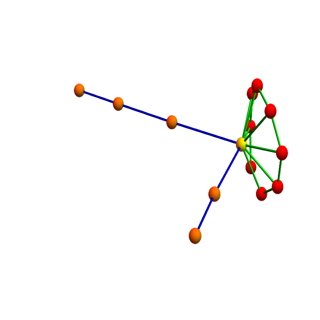
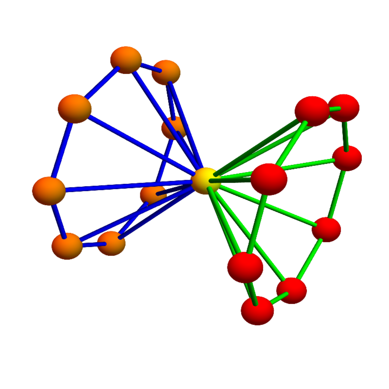
Lets look at the cubic valuation
summing over all triples of simplices which have a nonempty common intersection.
Examples.
1) In the case of with ,
there are already 175 possible ordered triples of non-intersecting complete
sub graphs like
2) The behavior of cubic valuations on complete graphs is the same than for . We have .
Theorem 16.
For -graphs with boundary and any even :
For any odd we have
Proof.
The proof bootstraps and uses that for a unit sphere . ∎
In other words, we know the Wu polynomial for graphs.
The examples of star illustrates how branch points produces quadratic growth in the number of branches. These numbers are of algebra-geometric nature as they go over to the continuum. Lets explain a bit more algebro-geometric relation.
12. Questions
A) Is the Wu characteristic the only multiplicative quadratic valuation on graphs
which assigns the value to points? Such a result was suggested by Wu in the 50ies and
Grünbaum cautioned in the 70ies to consider Dehn-Sommerville cases.
We know that the Euler characteristic is the only linear valuation on the category of finite
simple graphs which assigns the value to points. This fact has been proven a couple of times and
can be seen from the Barycentric refinement operator , which maps to
as it has only one eigenvalue and the eigenvector of is
leading to Euler characteristic.
While we understand the behavior of the -vector under Barycentric refinement,
we don’t understand yet the behavior of the -matrix under Barycentric refinement but
we have not looked yet really. In the case of Barycentric refinements, we have searched for
the law first by data fitting, proved it and then found it in the literature.
Any possible law should be detectable like that if it exists.
B) Assume we know all the multi-linear valuations of a graph. How much of the graph is
determined by these numbers? Are there non-graph isomorphic graphs with the property that all
-linear valuations are the same? Yes, if we restrict to the local valuations, we can already find
trees which are not isomorphic but have all valuations the same.
More difficult is to answer the question modulo homeomorphism equivalence [97] or even
homotopy. Can we get a complete set of invariants by relaxing the local property?
As the story of invariants for geometric objects has shown repetitively, it would be
surprising to have an exhaustive set of generalized valuations which are invariants. The
complexity of the graph isomorphism problem is not settled but it is not excluded yet that a
polynomial number of valuations together with maybe other numbers like spectra
suffice to determine the isomorphism type. History has shown that these are tough questions
and that even the search for counter examples can be computationally hard. Here is a quick
experiment: on all connected graphs of and vertices, linear and quadratic valuations determine
the isomorphism class uniquely (there are in the case of vertices and in the case of vertices).
But for vertices already, there are isomorphism classes of connected graphs but only
101 different linear and quadratic valuation patterns so that some graphs have the same pattern.
Including the cubic valuations already allows to distinguish isomorphism classes still missing .
Including quartic valuations still does not resolve more. Indeed, the following
two graphs with Stanley-Reiner ring elements and
have the same -forms for all degrees. We have
and
and the -cubic form is .
By the way, the two graphs have different Kirchhoff spectra.
C) Is there any significance of the -spectrum, the spectrum of the quadratic -form
defined by ? This spectrum is of course the same for isomorphic graph. Are there isospectral
graphs in the sense that they are not isomorphic but have the same -spectrum?
Is there a significance to the number of negative eigenvalues of ? Is there
a significance of the Perron-Frobenius eigenvector which always exist as is a positive matrix
if the graph is connected? What happens with the spectrum when applying
Barycentric refinements repetitively?
We have seen that the spectrum of the Laplacian etc converges
universally [103, 98]. The number of negative eigenvalues of the
-matrix varies from graph to graph. The star graph with 4 vertices
has the -matrix with
eigenvalues and . For all other star graphs is positive definite.
For circular graphs with , there is always one negative and positive eigenvalue.
For complete graph , the number of negative eigenvalues of is .
We see that in general the number of negative eigenvalues in the -spectrum can change if
undergoes a Barycentric refinement. For the -vector already, the inverse problem of characterizing
the possible -vectors is interesting. In the quadratic case we don’t know anything about the possible
-matrices.
D) For each valuation functional one can look at its variational problem: it is the problem to maximize or minimize among all graphs with vertices. When restricting to -graphs of a fixed number of vertices, maximizing volume is related to the upper bound conjecture. This shows that the problem of maximizing a general linear or quadratic valuation can be hard even in very intuitive cases. As for Euler characteristic, one can look at the expectation of the functional on Erdös-Renyi graphs. For any , we get so a function on . We can ask to maximize or minimize this. For , the utility graph is the only maximum and the maximal value of the Wu characteristic is . We have still to find a connected graph for which . Do such examples exist? Attaching hairs to 2-spheres shows that we can for any find graphs of vertices for which . Also for any , there are graphs of order with . Is it true that for any connected graph with vertices, the bound
holds for Wu characteristic? Monte Carlo experiments with smaller random graphs suggest
such an estimate to hold, but this can be misleading and be a case for the law of small
numbers. For Euler characteristic, where we know the expectation exactly on the Erdös-Renyi space
explicitly [82]. The expectation is
showing that there
is and arbitrary large graphs with vertices for which
despite the fact that we can not explicitly construct such examples. This might also happen
for the Wu characteristic.
E) Valuations can be studied from a statistical mechanics point of view. Define for every graph and a fixed function on edges of the intersection graph of simplices and fixed 0-form on the simplices the interaction energy
For a particular graph theoretical approach, see [16].
A simple case to look at , where and .
As notation from the Ising model is close, the spin values
of a simplex is geometrically defined and are all pairs of simplices which
intersect. As custom, one can then define a probability distribution function
on the Erdös-Rényi space of all graphs on a fixed vertex set,
where is the partition function. For any functional on graphs, there is a
mean value which could be studied in the limit .
One can also consider models where a host graph is fixed and exhausts it using natural sequences
of graphs. But unlike the Ising model, where the underlying graph is fixed
and the spin configurations are changed, the geometry alone determines the Wu energy. This renders
the story different. If we look at random Erdös-Rényi models, then we can look at the average Wu characteristic.
Unlike in the case of Euler characteristic, we were able to give an explicit formula for
the expectation value we don’t have an expectation for the Wu characteristic yet.
F) The Euler characteristic satisfies in full generality the Euler-Poincaré formula equating cohomological and combinatorial versions of the Euler characteristic
As noticed in [90], it was Benno Eckmann [38] appeared have
been the first to point out this connection in a purely discrete setting without
digressing to the continuum. An intriguing question is whether there is a cohomology
defined for general finite simple graphs which produces an Euler-Poincaré formula for
the quadratic Wu characteristic. It would have to be a sort of discrete intersection cohomology,
where a general finite simple graph now plays the role of a perverse sheaf. This is not so
remote, as finite simple graphs are an Abelian category which contain discretizations of
perverse sheaves. If a cohomology should exist which produces the Euler-Poincaré formula
for the Wu characteristic, then one can expect that its exterior derivative defines
an operator whose Laplacian produces a McKean-Singer formula equating
the Wu characteristic with the super trace of the heat kernel .
G) For -graphs with boundary, the formula
computes the Euler characteristic of the “virtual interior” chain of the graph.
This also works for complete graphs for which the Barycentric refinement is a d-ball.
For the triangle for example,
computes the Euler characteristic of the chain . Unlike graphs,
chains form a Boolean algebra and valuations are linear and nice. The category of graphs
is somehow like a manifold in the linear space of chains as adding two graphs throws us
out of the graph category. Lets write for the Boolean addition on the Boolean algebra
of chains. The addition is the symmetric difference on each simplex level.
The example shows that the sum is no more a graph.
The product which is the intersection on each dimension however is a graph.
The example shows how to
break up a triangle into two chains. The first is the boundary chain, the second is the interior chain.
But this decomposition is only possible in the ambient Boolean ring and not in the category of graphs.
As in the Stanley-Reisner picture (even so the multiplication in that ring is different),
the Euler characteristic the triangle as ,
the Euler characteristic of the boundary is ,
and the interior is . We see that the Wu characteristic
of is the Euler characteristic of the interior of and the same holds for a d-ball.
In [97] we defined a notion of homeomorphism for graphs which treats graphs as higher
dimensional structures which is compatible with homotopy, cohomology and dimension by design.
The topology of a graph is given by a base of subgraphs whose nerve is homotopic to the graph. We
have seen that such a topology always works and is given by the star graph.
This picture can now be generalized a bit by allowing the base to consist of virtual open balls.
H) This question is still under investigation: what happens with the -matrix of a graph if it undergoes Barycentric refinement ? As the -vector is transformed with a universal linear transformation, one can expect something similar to happen for the -matrix, or more generally for the intersection matrix for two intersecting graphs. If , then . For graphs without triangles, the -matrix is a symmetric matrix and there are three independent components. We can get the Barycentric refinement using linear algebra: as for a cycle graph we have , , we get and for the figure graph, we have . The transformation matrix can be found easily as
It has eigenavalues . At the moment, it looks as if this does not work any more for -dimensional graphs with clique number , where we look for a transformation matrix . For for example, we have mapping to reflecting the fact that the -matrix of is and the -matrix of its Barycentric refinement (a wheel graph with boundary) is . When trying to find a linear transformation relating the two -matrices using a set of 6 independent graphs, it does not work any more in general. There could be a possible on some subclasses of graphs, as there appear linear relations necessary. Also a nonlinear transformation rule can not yet be ruled out.
13. Conclusion
According to [17], there are two basic counting principle which underlie
most of arithmetic. It is that for two disjoint finite sets, and
. This fundamental structure is also present for graphs
and there is one quantity which in particular satisfies these properties. It is the
Euler characteristic. In this light, the Wu characteristics and its higher order versions
which were discussed here, are also fundamental as they satisfy both counting principles.
A quadratic valuation attaches to a pair of simplicial complexes a number such that and are both valuations. Similarly, as valuations are linear in the -vector where is the number of simplices of dimension , a quadratic valuation is a linear function on -quadratic forms , where is the number of simplices which are intersections of and dimensional simplices. The function in particular defines a functional on simplicial complexes which measures a self interaction energy. It does so especially for finite simple graphs equipped with the Whitney complex. An example of a quadratic valuation is the Wu characteristic [149] which sums over where is an ordered pair of complete subgraph of which have non-empty intersection. It is more subtle than Euler characteristic as unlike the later, the higher order Wu characteristics are not a homotopy invariant, and so is more subtle like the Bott invariant defined in or Reidemeister (analytic) torsion. We prove that is invariant under edge or Barycentric refinements, that it behaves additively with respect to connected sums and multiplicatively with respect to Cartesian products. We prove a Gauss-Bonnet formula for multi-linear valuations and use this to show that for a geometric graph with boundary , all the higher order Wu characteristic satisfy , where is the Euler characteristic. Simple examples like discrete curves show that the curvature is now nonlinear in the vertex degree. The setup allows to construct higher order Dehn-Sommerville relations, answering so positively a conjecture of Grünbaum [59] from 1970. The simplest example is the vanishing of the quadratic valuation with , where the quadratic -form counts the number of intersecting and subgraphs in a triangulation of a 4-manifold . More generally, we show that if is a Dehn-Sommerville invariant then the quadratic valuation is zero on -graphs. The lack of homotopy invariance is not a surprise, as most linear valuations already are not homotopy invariant. It is still not known whether the quadratic Wu invariant is the only quadratic invariant valuation on general graphs which is invariant under Barycentric refinement. For discrete curves, graphs without triangles for example, the curvature for Euler characteristic is while the curvature of the Wu characteristic is , where is the vertex degree at and the neighboring vertex degrees. Quadratic valuations also produce intersection numbers and are interesting for algebraic sets, where they produces combinatorial invariants for varieties which go beyond Euler characteristic as the quadratic Dehn-Sommerville curvatures at isolated singularities report on their internal structure.


Appendix: Code
More detailed code and examples can be obtained by downloading the LaTeX source file of this preprint on the ArXiv, then copy paste the Mathematica part from the file. We compressed the code as much as possible as shortness of code benefits both communication and verification. The Wolfram language is suitable to serve as pseudo code. Even if the language might evolve in the future, the following code should remain readable. Since Mathematica has not yet built in a procedure to list of all complete subgraphs in a graph, we do that first by hand. One can also use the iGraph library which uses compiled code and is faster. We don’t use it by default as this is a complex third party library. But the general problem is NP complete, so that one can not expect a very efficient algorithm.
Here is example code to compute the Euler characteristic Euler curvature entering Gauss Bonnet and Euler indices entering Poincaré-Hopf:
The following procedures compute the Wu characteristic and the cubic Wu Characteristic as well as the intersection number
Here are procedures to test the Gauss-Bonnet theorem for the Wu characteristic as well as the Poincaré-Hopf theorem for the Wu characteristic, two results proven in this paper:
Finally, here is an implementation of the graph product and Barycentric refinement. Unlike in the [101], where code for the procedure was algebraically given using the Stanley-Reisner ring, we perform the product here directly. We also have added an example line computing the Euler and Wu characteristics for two graphs and its product.
Here is the inductive dimension implementation for graphs. It is discussed in detail in [82]. It can also be used to illustrated the proven formula holding for any pair of graphs.
Here are procedures to compute the -vector or -matrix or -tensor in the cubic case of a graph:
Finally, lets look at some linear and multi-linear Dehn-Sommerville invariants. To test the produced we build a three or four dimensional sphere:
Like the category of sets, the category of graphs has addition and multiplication given by the symmetric difference and multiplication given by the intersection. But note that the ring product in the Stanley-Reiner ring uses a different multiplication which corresponds to a direct product of sets. Here is how to work with the basic Boolean algebra of graphs in the Wolfram language. Note that the built-in “GraphIntersection” procedure does not take the intersection of the vertex sets. The vertex list of with and is when using “GraphIntersection”. We therefore implement the procedure “GProduct”, which replaces that procedure and produces the true graph intersection which has a vertex set . Note that if and , then is not . The graph product of the two graphs and is while the intersection is . The sum of the two graphs is . On the vertex level this is not the symmetric difference of the vertex sets . Mathematica gives the zero dimensional three point graph as the graph intersection. Both the intersection as well as the Mathematica graph intersection do not honor distributivity. If modifying the product, we can salvage distributivity, but we still have situations where has a different graph with .
Appendix: Discrete Hadwiger
The following result of the discrete Hadwiger theorem parallels the statement for simplicial complexes proven in [79] (Theorem 3.2.4). The only change is vocabulary as it is formulated for subgraphs rather than general sub simplicial complexes. But the graph case is not new because the set of subgraphs of a graph defines a lattice , where is the empty graph and a linear valuation is a valuation on that lattice. The set of complete subgraphs in is then a generating set of this lattice and is the bottom element in this distributive lattice.
Theorem 17 (Discrete Hadwiger).
The vector space of invariant valuations on a finite simple graph is equal to the clique number of . A basis is given by the valuations counting the number of subgraphs in and where .
Proof.
We have to show that (i) the functionals are linearly independent and (ii) that every valuation
a linear combination of the functionals .
(i) Assume that we can find a vector such
that
for all subgraphs of .
By taking complete subgraphs we see that is perpendicular to the vectors
.
Since all these vectors are linearly independent for , the vector must be zero.
Barycentric refinement gives an algebraic proof of linear independence as the eigenfunctions of ,
where is the Barycentric refinement operator are linearly independent as the
matrix has different eigenvalues for .
(ii) Given an arbitrary invariant valuation on . By the invariance property in the definition, there is for every a real number such that for all complete subgraphs of dimension . Also by definition. Define now . Since every subgraph of can be written as a union of complete subgraphs and both , we can use the inclusion-exclusion property to see inductively that . ∎
This can be generalized to higher dimensions. Lets just discuss the quadratic case:
Theorem 18 (Hadwiger for quadratic valuations).
The vector space of quadratic valuations has dimension .
Proof.
The proof is very similar. One has to get an independent set of valuations and then show that every valuation can be written as a linear combination of this set. Lets look at the valuation measuring the number of -simplices intersecting with -simplices in . This number grows like under Barycentric subdivision. These are growth rates which are independent. To show that these number span, note that every quadratic valuation can be written as with . ∎
For example, for , the set of quadratic valuations is , it is the valuation
which counts the discrete set of points. In the one dimensional case , there
the valuation space is dimensional, we look at the number of vertices, the
number of pairs of edges intersecting and the number of vertex-edge pairs, which is
twice the number of edges.
In the continuum, one restricts the theory of valuations to convex sets
or polyconvex sets, which is a term introduced in [79] and
means a finite union of convex sets in . Also polyconvex sets form
a lattice. Things are related of course as any finite simple graph has
a geometric realization in which it is a polyconvex set. The fact that in graph theory,
the values form a basis of all valuations can also be seen as a
manifestation of the Groemer extension theorem from a generating set
to the full lattice.
The structure of valuations on discrete spaces is much richer than the structure of measures.
Note that on a finite set , there is only a -dimensional space of
measures if we ask the measure to be invariant. It is a multiple of the counting measure,
which is the Haar measure with respect to the symmetric group acting on .
So, thinking about a valuation as a measure is somewhat misleading.
On a finite set, there is a natural algebra, the set of all subsets and the structure
of all signed measures on this algebra is a dimensional space given by all
, a trivial manifestation of the Riesz representation theorem
applied to linear functionals on the set of continuous functions
which happens to adopt even a Hilbert space structure in the
finite case. The fact that set of measures invariant under permutations is
-dimensional settles the theory of invariant measures on a finite set.
On the other hand, if the discrete set is quipped with a graph structure and the
corresponding simplicial complex,
the theory of valuations is more interesting, as the Hadwiger theorem illustrates.
The theory of measures does not look at the internal structure of the sets
which are measured, unlike the theory of valuations which look inside. In the continuum,
it is a bit harder to explore this internal structure as one needs tomographic methods,
but the language of probability theory like Crofton or kinematic formulas allow to deal with it.
As we have hoped to demonstrate in this article, some interesting mathematics in discrete differential geometry
like Gauss-Bonnet, or Poincaré-Hopf can be seen naturally as results on valuations. We
also hoped to show that the language of graphs works well also to discover new results.
Working with subgraphs of a graph is a bit like working with subsets but hides the difficulty
that the theory of valuations really does more: it deals with the distributive lattice of
simplicial subcomplexes of a given simplicial complex rather than the lattice of
subsets of a given set. But working with sets of subsets as the basic structure is
harder to think and write about. The language of graphs is more intuitive similarly as the
concept of metric topologies is easier to deal with than arbitrary topologies.
The analogy between discrete Hadwiger and continuous Hadwiger is so close that one might wonder whether it is possible to treat them in a unified manner. This is indeed possible as emerged while working with Barry Tng [146] ind we sketch the connection: a measure on the set of linear functions on defines a length on smooth parametrized curves by the Crofton formula: take smooth random linear function with equidistant level surfaces and produce the random variable counting the number of intersections with the curve. The law of large numbers shows that the expectation of this random variable can be explored by a Monte Carlo computation. It defines a length functional on curves, the property that it is additive is related to the additivity of probability. We have now only a semi-metric on but the Kolmogorov quotient is now a metric space. The Kolmogorov quotient just takes equivalence classes of points for which the semimetric is zero. For the semi metric in the plane for exmple, the Kolmogorov quotint is the real line. If is a measure which is invariant under translations and rotations, then it recovers the usual metric on up to a scaling factor. This is the Crofton formula which for polygons reduces to the Buffon needle computation. If is a finite point measure, then the Kolmogorov quotient is a finite graph. This setup is rather general and most conveniently described in the projective situation, where translation is part of the projective group. Any compact Riemannian manifold can be treated like that: Nash embed it into some projective space , look at the Haar measure on all linear functions on invariant under projective transformations. Then, as the arc length on curves in is the same than arc length on , we can look at the measure on the set of Morse functions on given by the push forward of the Haar measure on linear functions to the space of Morse functions on . This defines now a probability space on the class of Morse functions on which allows to recover the Riemannian metric integral-geometrically within the manifold . The point is however that by choosing a different measure on Morse functions, we get different metric spaces. In particular, if we take a discrete finite point measure, we get a discrete space. Going back to the case , the probability space is a set of linear functions, we have convex sets obtained by inequalities . Why does the dimension of valuations in agree with the dimension of valuations on graphs? For any finite measures we have a -dimensional set of valuations by discrete Hadwiger. Now approximate the original Haar measure with finite measures leading to -dimensional graphs by doing Barycentric subdivisions, we can get to the Haar measure. Since valuations go over to the limit and the dimension of the set of valuations is upper semi continuous, the discrete approximation argument shows that we have at least a -dimensional set of valuations in the continuum. We can also go backwards and approximate a given discrete finite measure by absolutely continuous measures. Assume that the vector space of valuations is -dimensional with . We would get different valuations in the discrete limit which is not the case. On simplices we can compute the ’th valuation by adding up the -dimensional measures of -dimensional subsimplices. On convex subsets , we can make a triangulation and sufficiently many Barycentric subdivisions in Euclidean space allowing to compute the valuation numerically by adding up the valuations on subsimplices. Smooth manifolds allowing an approximation by polytopes, the valuation is still defined as a limit. The setup is much more than just a unification the theory of valuations on Euclidean space or graphs. We can see that for any measure , which even might be singular continuous, we get to geometric spaces which have a Hadwiger theorem. These spaces can be objects with fractal dimension. They can be seen as approximations of graphs or then as limiting cases of smooth manifolds. The more general setup can use to make sense of curvature also on more general spaces as we can define curvature integral geometrically. We can use the function to define an index at a point and use the measure to average this index to get a curvature function . While we have not gone into this general framework here and stayed strictly within graph theory, we hope that the prospect of a much more general geometry which includes both graph theory as well as Riemannian geometry, makes the graph theoretical setup more relevant.
Appendix: About the literature
The results are formulated in the language of graph theory [18, 9, 10] which itself has various topological graph theory [58] or algebraic graph theory [15]. There is overlap with work on polytopes [153, 60], simplicial complexes [141, 142, 72] or combinatorial topology like [61, 138]. See [37] for history. Various flavors of discrete topologies have emerged: digital topology [108, 62, 41], discrete calculus [56], Fisk theory [2, 45, 43, 44, 46] to which we got in the context of graph colorings [96, 99] leading to the notion of spheres which appeared in [40] which is based on homotopy [69, 24], based on notions put forward in [75, 150], networks [121, 120, 147, 28, 121, 147, 68], physics [35, 129, 31, 53, 117, 134], computational geometry [36, 12, 34, 123, 151] discrete Morse theory [47, 48, 49, 51], eying classical Morse theory [114], discrete differential geometry in relation to classical differential geometry [13, 54, 74]. We got to into the subject through [84] and generalized it to [83] and summarized in [89] after [85]. The general Gauss-Bonnet-Chern result appeared in [83] but was predated in [109]. It seems Gauss-Bonnet for graphs has been rediscovered a couple of times like [70, 50]. We noticed the first older appearance [70] in [100] and found [109, 50] while working on the present topic. Various lower dimensional versions of curvature have appeared [57, 126, 127, 64, 119, 145]. The first works on Gauss-Bonnet in arbitrary dimensions include [66, 4, 42, 3, 25, 26]. For modern proofs, see [32, 132]. The story of Euler characteristic is told in [52, 130, 111]. A historical paper is [39]. For uniqueness of Euler characteristic as a linear valuation see [80, 133, 70, 50, 131, 152, 110]. For Hadwiger’s theorem of 1957, see [79, 78]. The first works on Poincaré-Hopf were [124, 66, 116]. For more history, see [139, 115, 19, 55, 65]. Poincaré-Hopf indices are central in discrete approaches to Riemann-Roch [6, 5]. The index expectation result is [87]. The closest related work is Banchoff [8, 7]. For integral geometry and geometric probability, see [79, 135]. It is a popular topic for REU research projects like [22]. The index formula for Euler characteristic appeared in [86] which proves a special case of the result here along the same lines. See also [92] for the recursion. The Sard approach in [102] simplified this. That paper gives a discrete version of [136]. We got into the Barycentric invariants through [98, 103] after introducing a graph product [101] which was useful in [100], a paper exploring topology of graphs [97, 73, 90]. Originally we were interested in the spectral theory of graphs [27, 128, 1, 33, 125, 144] which parallels the continuum [23, 132, 13]. The linear algebra part of networks was explored in [88] which is a discrete version of [113]. See also [91, 95, 94, 93, 104, 106] and [67, 112] for discrete combinatorial Laplacians. For the Dehn-Sommerville relations, see [81, 122, 118, 110, 21, 63, 77]. In [122, 77] appear Dehn-Sommerville-Klee equations for discrete for manifolds with boundary. In [110], it was noted that the Euler characteristic is the only invariant, using the operator . The combinatorics of the Barycentric operator was studied in[11] in the case . The explicit formula using Stirling numbers appeared in [21]. For Polytopes [36, 130, 137, 29, 60, 71, 107, 30]. The theory of valuations on distributive lattices has been pioneered by Klee [80] and Rota [133] who proved that there is a unique valuation such that for any join-irreducible element. This is the Euler characteristic. The example of the lattice of subgraphs of a graph fits within this framework.
Appendix: Summaries
The next two pages are from October 2, 2015. The new results are then added where indicated.
Originally we used the central manifolds to argue the vanishing of the Barycentric invariant numbers.
There were too statements which overreached in the October 2 summary:
the symmetric index is not always constant zero for Dehn-Sommerville valuations.
Also, the index expectation does not generalize without modifications from Euler characteristic
to general valuations. The index formula still produces probabilistic statements about random
geometric subgraphs of spheres, but these results still need to be harvested.
If is the category of finite simple graphs , the linear space of valuations on has a basis given by the -numbers counting complete subgraphs in . The barycentric refinement of is the graph with subgraphs as vertex set where new vertices are connected if or . Under refinement, the clique data transform as with the upper triangular matrix with Stirling numbers . The eigenvectors of with eigenvalues form an other basis in . The are normalized so that the first nonzero entry is and all entries are in with no common prime factor. is the Euler characteristic , the homotopy and so cohomology invariant on . Half of the will be zero Dehn-Sommerville-Klee invariants like half the Betti numbers are redundant under Poincaré duality. On the set with clique number , the valuations have dimension by discrete Hadwiger. A basis is the eigensystem of the submatrix matrix of . The functional is volume, counting the facets of . For , define and as the number of complete subgraphs of the unit sphere , the graph generated by the neighbors of . The fundamental theorem of graph theory is the formula . For , it is the Euler’s handshake. For a valuation , define curvature . Generalizing the fundamental theorem:
Theorem (Gauss-Bonnet).
.
Example. For an icosahedron with and , we have
, , ,
, , ,
, , .
Let be the set of colorings of , locally injective function on . The unit ball at is the graph generated by the union of and the unit sphere which is the boundary . For and define the index , where and . It is local and a divisor. Inductive attaching vertices gives:
Theorem (Poincaré-Hopf).
.
Let be a Borel probability measure on and its expectation. Let be the chromatic number of . Assume either that is the counting measure on the finite set of colorings of with real colors or that is a product measure on for which functions with are independent identically distributed random variables with continuous probability density function. For all and :
Theorem (Banchoff index expectation).
For Euler characteristic .
The empty graph is a -graph and -sphere. Inductively, a -graph is a for which the unit spheres are -spheres. An Evako -sphere is a -graph which when punctured becomes contractible. Inductively, is contractible if there exists such that both and the graph without are contractible. The graph is contractible. Given and , define the graph in the refinement of consisting of vertices, where changes sign. In that case, at every vertex , there is a -graph defined as the level surface in . The next Sard result belongs to discrete multivariable calculus:
Theorem (Implicit function theorem).
For a -graph and and , the hyper surface is a -graph.
The symmetric index of at is defined as
Theorem (Index formula).
For and Euler characteristic, then
Poincaré-Hopf allows fast recursive computation of for most in quantified using Erdös-Renyi measures. For -graphs, the symmetric index is is if is odd and if is even. If is even, we have , as curvature is supported on . Furthermore, we have if .
Theorem (Dehn-Sommerville-Klee).
For a -graph and even , the functions are supported on . If , then .
with even span classical invariants.
Zero curvature for all also follows
from Gauss-Bonnet and suspension.
Curvature functionals are linear combination of Barycentric functionals for .
The classical DS-invariants in dimension can be derived from Gauss-Bonnet and
the fact that curvatures are DS-invariants in dimension d-1.
Illustration:
on 4-graphs shows that a 4-graph triangulation
of a compact 4-manifold with vertices, edges,
triangles, tetrahedra, and pentatopes satisfies . Examples:
for the 4-crosspolytop , a 4-sphere with , we get
. For a discrete , a product graph
constructed using the Stanley-Reisner ring, with
, we get .
For a discrete with ,
we get .
This ends the summary from October 2. Here is is a summary of what has been found since
written in a compressed form.
A -linear valuation is a real valued map on ordered tuples of subgraphs
such that each is a linear valuation, a map from the
set of subgraphs satisfying and .
Given two valuations , the quadratic valuation is an example.
We assume them to be localized in the sense if .
A -linear valuation defines a nonlinear valuation .
Of special interest are quadratic valuations which can be seen as intersection numbers.
Every linear valuation which is invariant in the sense that for isomorphic graphs
defines a linear map on -vectors . The linear map is represented by
a -vector like . We have then .
If is the quadratic -form, where counts how many simplces in
intersect in a non-empty set with a simplex in . We especially have the -matrix
which encodes the intersections of simplices in . A quadratic valuation can
now be given by two vectors : one has
or . An example is the Wu characteristic
. Similarly, one can define -linear valuations and have
the higher Wu characteristic . By Hadwiger, the space of linear valuations
is dimensiona, the space of quadratic valuations dimensional
with not yet known dimension.
Given two finite simple graphs , define a new graph as follows: assume the vertex sets of are disjoint. The vertex set of consists of all pairs with being a simplex in and being a simplex in . Two such elements are connected by an edge, if one is contained in the other. For a finite simple graph , the product is called the Barycentric refinement of . It has the set of simplices of as vertices and two simplices connected if one is contained in the other. The addition of two graphs is defined as the disjoint union of the two graphs. Note that is only associative, when the product is describe algebraically as the product in the Stanley-Reisner ring. The following four theorems hold in the class of all finite simple graphs:
Theorem (Gauss-Bonnet).
Every -linear valuation has a curvature defined on vertices of such that .
Lets elaborate a bit in the case of quadratic valuations: By definition , where only depend on the dimensions of and . There are two vectors such that using the quadratic -form , we have . To get the curvature, write with . Now distribute the value of equally to all of the vertices of . This gives the curvature function on vertices.
Theorem (Poincaré-Hopf).
For every -linear valuation and any locally injective scalar function on the vertices of , there is an index such that .
Given a valuation , its Poincaré-Hopf index is defined as
where is the graph generated by and is the graph generated by . For the same type of probability measures as in the linear case, we have:
Theorem (Index expectation).
The expectation of over the probability space of functions is the curvature .
As for linear valuations, a deformation of the probability measure on functions (like for example given by a wave evolution) changes the curvature but keeps Guass-Bonnet intact. The deformation of the probability measure allows for other type of curvatures.
Theorem (Topological Invariants).
Every Wu characteristic is invariant under Barycentric refinements.
Since , we can see as a sum of values of a function on the vertex set of the Barycentric refinement . This function is an index for a natural ordering of the vertices of .
Theorem (Multiplicative function).
Every Wu characteristic is multiplicative .
To illustrate the quadratic case, first show for simplices
then write , finally uses the Barycentric
invariance.
The following two theorems hold only for -graphs or -graphs with boundary:
Theorem (Boundary formula).
For every -graph with boundary , we have .
For -graphs without boundary this is shown by verifying that the Wu curvature and Euler curvatures agree. What happens at the boundary is that for simplices hitting the boundary there is an additional contribution one or minus one. The corresponding sum is the Euler characteristic of a thickend boundary which is homotopic to the actual boundary.
Theorem (Grünbaum question).
For every -graph without boundary and every linear valuation , the quadratic valuation satisfies .
This could be generalized to -linear cases. Like that and the cubic valuation agree up to a sign on the graph . The proof goes by writing the valuation as a sum over pairs of intersecting simplices and then partition according to which simplex they intersect. When looking at a sum for fixed , then the part of the interacting simplices is zero. This uses that any lower dimensional spheres have the correct Euler characteristic.
Theorem (Dehn Sommerville space).
The Dehn-Sommerville space of -valuations has the same dimension as the Dehn-Sommerville space of linear valuations .
The fact that the Dehn-Sommerville valuations are linearly independent follows from the fact that there is a basis given by eigenvectors to different eigenvalues. An alternative basis are the classical Dehn-Sommerville valuations
There can not be a larger dimensional space of valuations since a simple example of cross polytopes obtained by doing multiple suspension of a circular graph shows that only can be zero in general. For some graphs of course, the space of valuations which vanish can be larger. An example is the 2-torus for which the -matrix is
The Dehn-Sommerville space of the 2-torus is -dimensional.
For dimensional graphis we have only a -dimensional Dehn-Sommerville space.
By the way, with , then and the Wu invariant is
as the Wu characteristic is the Euler characteristic, which is
for the 2-torus.
Finally, Gauss-Bonnet for linear valuations immediately shows that
Theorem.
Flatness of D-S For any -graph and Dehn-Sommerville relation, and is flat in the sense that all curvatures are constant zero.
The proof uses that curvature at a vertex is a Dehn-Sommerville valuation of the unit sphere of the graph at .
References
- [1] W.H. Haemers A.E. Brouwer. Spectra of graphs. Springer, 2010.
- [2] M.O. Albertson and W.R. Stromquist. Locally planar toroidal graphs are -colorable. Proc. Amer. Math. Soc., 84(3):449–457, 1982.
- [3] C. Allendoerfer and A. Weil. The gauss-bonnet theorem for riemannian polyhedra. Transactions of the American Mathematical Society, 53:101–129, 1943.
- [4] C.B. Allendoerfer. The Euler number of a Riemann manifold. Amer. J. Math., 62:243, 1940.
- [5] M. Baker and S. Norine. Riemann-Roch and Abel-Jacobi theory on a finite graph. Advances in Mathematics, 215:766–788, 2007.
- [6] M. Baker and S. Norine. Harmonic morphisms and hyperelliptic graphs. International Mathematics Research Notices, pages 2914–2955, 2009.
- [7] T. F. Banchoff. Critical points and curvature for embedded polyhedral surfaces. Amer. Math. Monthly, 77:475–485, 1970.
- [8] Thomas Banchoff. Critical points and curvature for embedded polyhedra. J. Differential Geometry, 1:245–256, 1967.
- [9] B.Bollobás. Modern Graph Theory. Graduate Texts in Mathematics. Springer, New York, 1998.
- [10] B.Bollobás. Random graphs, volume 73 of Cambridge Studies in Advanced Mathematics. Cambridge University Press, Cambridge, second edition, 2001.
- [11] M. Begue, D.J. Kelleher, A. Nelson, H. Panzo, R. Pellico, and A. Teplyaev. Random walks on barycentric subdivisions and the Strichartz hexacarpet. Exp. Math., 21(4):402–417, 2012.
- [12] M.de Berg, M.van Kreveld, M.Overmars, and O.Schwarzkopf. Computational Geometry. Springer Verlag, second edition, 1998.
- [13] M. Berger. A Panoramic View of Riemannian Geometry. Springer Verlag, Berlin, 2003.
- [14] M. Berger. Jacob’s Ladder of Differential Geometry. Springer Verlag, Berlin, 2009.
- [15] N. Biggs. Algebraic Graph Theory. Cambridge University Press, 1974.
- [16] N.L. Biggs. Interaction models, volume 30 of London Mathematical Society Lecture Note Series. Cambridge University Press, 1977.
- [17] N.L. Biggs. The roots of combinatorics. Historia Mathematica, 6:109–136, 1979.
- [18] J. Bondy and U. Murty. Graph theory, volume 244 of Graduate Texts in Mathematics. Springer, New York, 2008.
- [19] B.O’Neill. Elementary Differential Geometry. Elsevier, revised second edition, 2006.
- [20] R. Bott. Two new combinatorial invariants for polyhedra. Portugaliae Math., 11:35–40, 1952.
- [21] F. Brenti and V. Welker. -vectors of barycentric subdivisions. Math. Z., 259(4):849–865, 2008.
- [22] R.K. Johnson C.E. Csar and R.Z. Lamberty. Geometric valuations. REU Project university of Notre Dame.
- [23] I. Chavel. Eigenvalues in Riemannian Geometry. Pure and applied mathematics. Academic Press Inc., Orlando, 1984.
- [24] B. Chen, S-T. Yau, and Y-N. Yeh. Graph homotopy and Graham homotopy. Discrete Math., 241(1-3):153–170, 2001. Selected papers in honor of Helge Tverberg.
- [25] S.-S. Chern. A simple intrinsic proof of the Gauss-Bonnet formula for closed Riemannian manifolds. Annals of Mathematics, 45, 1944.
- [26] S-S. Chern. Historical remarks on Gauss-Bonnet. In Analysis, et cetera, pages 209–217. Academic Press, Boston, MA, 1990.
- [27] F. Chung. Spectral graph theory, volume 92 of CBMS Regional Conf. Series. AMS, 1997.
- [28] R. Cohen and S. Havlin. Complex Networks, Structure, Robustness and Function. Cambridge University Press, 2010.
- [29] H.S.M. Coxeter. Regular Polytopes. Dover Publications, New York, 1973.
- [30] P.R. Cromwell. Polyhedra. Cambridge University Press, 1997.
- [31] K.S. Thorne C.W. Misner and J.A. Wheeler. Gravitation. Freeman, San Francisco, 1973.
- [32] H.L. Cycon, R.G.Froese, W.Kirsch, and B.Simon. Schrödinger Operators—with Application to Quantum Mechanics and Global Geometry. Springer-Verlag, 1987.
- [33] Y.Colin de Verdière. Spectres de Graphes. Sociéte Mathématique de France, 1998.
- [34] M. Desbrun, E. Kanso, and Y. Tong. Discrete differential forms for computational modeling. In A. Bobenko, P. Schroeder, J. Sullivan, and G. Ziegler, editors, Discrete Differential Geometry, Oberwohlfach Seminars, 2008.
- [35] M. Desbrun and K. Polthier. Discrete differential geometry: An applied introduction. In Ari Stern Peter Schröder, Eitan Grinspun, editor, SIGGRAPH 2006, 2006.
- [36] S. Devadoss and J. O’Rourke. Discrete and Computational Geometry. Princeton University Press, 2011.
- [37] J. Dieudonne. A History of Algebraic and Differential Topology, 1900-1960. Birkhäuser, 1989.
- [38] B. Eckmann. The Euler characteristic - a few highlights in its long history. In Mathematical Survey Lectures: 1943-2004, 1999.
- [39]
L. Euler.
Letter to Goldbach of 14. November, 1750
. http://eulerarchive.maa.org/correspondence/letters/OO0863.pdf, 1750. - [40] A.V. Evako. Dimension on discrete spaces. Internat. J. Theoret. Phys., 33(7):1553–1568, 1994.
- [41] A.V. Evako. The Jordan-Brouwer theorem for the digital normal n-space space . http://arxiv.org/abs/1302.5342, 2013.
- [42] W. Fenchel. On total curvatures for riemannianm manifolds (i). J. London Math. Soc, 15:15, 1940.
- [43] S. Fisk. Geometric coloring theory. Advances in Math., 24(3):298–340, 1977.
- [44] S. Fisk. Variations on coloring, surfaces and higher-dimensional manifolds. Advances in Mathematics, pages 226–266, 1977.
- [45] S. Fisk. The nonexistence of colorings. Journal of Combinatorial Theory B, 24:247–2480, 1978.
- [46] S. Fisk. Cobordism and functoriality of colorings. Adv. in Math., 37(3):177–211, 1980.
- [47] R. Forman. A discrete Morse theory for cell complexes. In Geometry, topology, and physics, Conf. Proc. Lecture Notes Geom. Topology, IV, pages 112–125. Int. Press, Cambridge, MA, 1995.
- [48] R. Forman. Morse theory for cell complexes. Adv. Math., page 90, 1998.
- [49] R. Forman. Combinatorial differential topology and geometry. New Perspectives in Geometric Combinatorics, 38, 1999.
- [50] R. Forman. The Euler characteristic is the unique locally determined numerical invariant of finite simplicial complexes which assigns the same number to every cone. Discrete Comput. Geom, 23:485–488, 2000.
- [51] R. Forman. Bochner’s method for cell complexes and combinatorial ricci curvature. Discrete Comput. Geometry, pages 323–374, 2003.
- [52] C. Francesex and D. Richeson. The flaw in Euler’s proof of his polyhedral formula. Amer. Math. Monthly, 114(4):286–296, 2007.
- [53] J. Fröhlich. Regge calculus and discretized gravitational functional integrals. In Advanced Series in Mathematical Physics, volume 15. World Scientific, 1981.
- [54] S. Gallot, D.Hulin, and J.Lafontaine. Riemannian geometry. Springer-Verlag, Berlin, second edition, 1990.
- [55] D. Gottlieb. All the way with Gauss-Bonnet and the sociology of mathematics. Amer. Math. Monthly, 103(6):457–469, 1996.
- [56] L.J. Grady and J.R. Polimeni. Discrete Calculus, Applied Analysis on Graphs for Computational Science. Springer Verlag, 2010.
- [57] M. Gromov. Hyperbolic groups. In Essays in group theory, volume 8 of Math. Sci. Res. Inst. Publ., pages 75–263. Springer, 1987.
- [58] J.L. Gross and T.W. Tucker. Topological Graph Theory. John Wiley and Sons, 1987.
- [59] B. Grünbaum. Polytopes, graphs, and complexes. Bull. Amer. Math. Soc., 76:1131–1201, 1970.
- [60] B. Grünbaum. Convex Polytopes. Springer, 2003.
- [61] A. Hatcher. Algebraic Topology. Cambridge University Press, 2002.
- [62] G.T. Herman. Geometry of digital spaces. Birkhäuser, Boston, Basel, Berlin, 1998.
- [63] G. Hetyei. The Stirling polynomial of a simplicial complex. Discrete and Computational Geometry, 35:437–455, 2006.
- [64] Y. Higuchi. Combinatorial curvature for planar graphs. J. Graph Theory, 38:220–229, 2001.
- [65] M.W. Hirsch. Differential topology. Graduate texts in mathematics. Springer-Verlag, Berlin, 1976.
- [66] H. Hopf. Über die Curvatura integra geschlossener Hyperflaechen. Mathematische Annalen, 95:340–367, 1926.
- [67] D. Horak and J. Jost. Spectra of combinatorial Laplace operators on simplicial complexes. Adv. Math., 244:303–336, 2013.
- [68] O.C. Ibe. Fundamentals of Stochastic Networks. Wiley, 2011.
- [69] A. Ivashchenko. Contractible transformations do not change the homology groups of graphs. Discrete Math., 126(1-3):159–170, 1994.
- [70] A.V. Ivashchenko. Graphs of spheres and tori. Discrete Math., 128(1-3):247–255, 1994.
- [71] C. Goodman-Strauss J.H. Conway, H.Burgiel. The Symmetries of Things. A.K. Peterse, Ltd., 2008.
- [72] J. Jonsson. Simplicial Complexes of Graphs, volume 1928 of Lecture Notes in Mathematics. Springer, 2008.
- [73]
F. Josellis and O. Knill.
A Lusternik-Schnirelmann theorem for graphs.
http://arxiv.org/abs/1211.0750, 2012. - [74] J. Jost. Riemannian Geometry and Geometric Analysis. Springer Verlag, 2005.
- [75] II J.W. Alexander. A proof of the invariance of certain constants of analysis situs. Trans. Amer. Math. Soc., 16(2):148–154, 1915.
- [76] G. Kalai. A simple way to tell a simple polytope from its graph. J. Combin. Theory Ser. A, 49(2):381–383, 1988.
- [77] D. Klain. Dehn-sommerville relations for triangulated manifolds. http://faculty.uml.edu/dklain/ds.pdf, 2002.
- [78] D.A. Klain. A short proof of hadwiger’s characterization theorem. Mathematika, 42:329–339, 95.
- [79] D.A. Klain and G-C. Rota. Introduction to geometric probability. Lezioni Lincee. Accademia nazionale dei lincei, 1997.
- [80] V. Klee. The euler characteristic in combinatorial geometry. The American Mathematical Monthly, 70(2):pp. 119–127, 1963.
- [81] V. Klee. A combinatorial analogue of poincare’s duality theorem. Canadian J. Math., 16:517–531, 1964.
- [82]
O. Knill.
The dimension and Euler characteristic of random graphs.
http://arxiv.org/abs/1112.5749, 2011. - [83]
O. Knill.
A graph theoretical Gauss-Bonnet-Chern theorem.
http://arxiv.org/abs/1111.5395, 2011. - [84] O. Knill. A discrete Gauss-Bonnet type theorem. Elemente der Mathematik, 67:1–17, 2012.
- [85]
O. Knill.
A graph theoretical Poincaré-Hopf theorem.
http://arxiv.org/abs/1201.1162, 2012. - [86]
O. Knill.
An index formula for simple graphs .
http://arxiv.org/abs/1205.0306, 2012. - [87]
O. Knill.
On index expectation and curvature for networks.
http://arxiv.org/abs/1202.4514, 2012. - [88]
O. Knill.
The McKean-Singer Formula in Graph Theory.
http://arxiv.org/abs/1301.1408, 2012. - [89]
O. Knill.
The theorems of Green-Stokes,Gauss-Bonnet and Poincare-Hopf in Graph
Theory.
http://arxiv.org/abs/1201.6049, 2012. - [90] O. Knill. A Brouwer fixed point theorem for graph endomorphisms. Fixed Point Theory and Applications, 85, 2013.
- [91]
O. Knill.
The Dirac operator of a graph.
http://http://arxiv.org/abs/1306.2166, 2013. - [92]
O. Knill.
The Euler characteristic of an even-dimensional graph.
http://arxiv.org/abs/1307.3809, 2013. - [93]
O. Knill.
An integrable evolution equation in geometry.
http://arxiv.org/abs/1306.0060, 2013. - [94]
O. Knill.
Isospectral deformations of the dirac operator.
http://arxiv.org/abs/1306.5597, 2013. - [95]
O. Knill.
Classical mathematical structures within topological graph theory.
http://arxiv.org/abs/1402.2029, 2014. - [96] O. Knill. Coloring graphs using topology. http://arxiv.org/abs/1410.3173, 2014.
- [97]
O. Knill.
A notion of graph homeomorphism.
http://arxiv.org/abs/1401.2819, 2014. - [98]
O. Knill.
The graph spectrum of barycentric refinements.
http://arxiv.org/abs/1508.02027, 2015. - [99] O. Knill. Graphs with Eulerian unit spheres. http://arxiv.org/abs/1501.03116, 2015.
- [100]
O. Knill.
The Jordan-Brouwer theorem for graphs.
http://arxiv.org/abs/1506.06440, 2015. - [101]
O. Knill.
The Künneth formula for graphs.
http://arxiv.org/abs/1505.07518, 2015. - [102]
O. Knill.
A Sard theorem for graph theory.
http://arxiv.org/abs/1508.05657, 2015. - [103]
O. Knill.
Universality for barycentric subdivision.
http://arxiv.org/abs/1509.06092, 2015. - [104]
O. Knill.
The zeta function for circular graphs.
http://arxiv.org/abs/1312.4239, December 2013. - [105] O. Knill and T. Tucker. A Riemann-Hurwitz theorem in graph theory. Draft Notes, December 2012.
- [106] Oliver Knill. Cauchy-Binet for pseudo-determinants. Linear Algebra Appl., 459:522–547, 2014.
- [107] I. Lakatos. Proofs and Refutations. Cambridge University Press, 1976.
- [108] V. Neumann Lara and R.G. Wilson. Digital Jordan curves—a graph-theoretical approach to a topological theorem. Topology Appl., 46(3):263–268, 1992. Special issue on digital topology.
- [109] N. Levitt. The Euler characteristic is the unique locally determined numerical homotopy invariant of finite complexes. Discrete Comput. Geom., 7:59–67, 1992.
- [110] A. Luzon and M.A. Moron. Pascal triangle, Stirling numbers and the unique invariance of the euler characteristic. arxiv.1202.0663, 2012.
- [111] J. Malkevich. Euler’s polyhedral formula I,II. AMS feature articles, 2004-2005. http://www.ams.org/samplings/feature-column/fcarc-eulers-formulaii.
- [112] T. Mantuano. Discretization of Riemannian manifolds applied to the Hodge Laplacian. Amer. J. Math., 130(6):1477–1508, 2008.
- [113] H.P. McKean and I.M. Singer. Curvature and the eigenvalues of the Laplacian. J. Differential Geometry, 1(1):43–69, 1967.
- [114] J. Milnor. Morse theory, volume 51 of Annals of Mathematics Studies. Princeton University press, Princeton, New Jersey, 1963.
- [115] J. Milnor. Topology from the differential viewpoint. University of Virginia Press, Charlottesville, Va, 1965.
- [116] M. Morse. Singular points of vector fields under general boundary conditions. American Journal of Mathematics, 51, 1929.
- [117] P. Mullen, A. McKenzie, D. Pavlov, L. Durant, Y. Tong, E. Kanso, J. E. Marsden, and M. Desbrun. Discrete Lie advection of differential forms. Found. Comput. Math., 11(2):131–149, 2011.
- [118] S. Murai and I. Novik. Face numbers of manifolds with boundary. http://arxiv.org/abs/1509.05115, 2015.
- [119] O. Narayan and I. Saniee. Large-scale curvature of networks. Physical Review E, 84, 2011.
- [120] Mark Newman, Albert-László Barabási, and Duncan J. Watts, editors. The structure and dynamics of networks. Princeton Studies in Complexity. Princeton University Press, Princeton, NJ, 2006.
- [121] M.E.J. Newman. Networks. Oxford University Press, Oxford, 2010. An introduction.
- [122] I. Novik and E. Swartz. Applications of Klee’s Dehn-Sommerville relations. Discrete Comput. Geom., 42(2):261–276, 2009.
- [123] R. Rieben P. Castilo, J. Koning and D. White. A discrete differential forms framework for computational electromagnetism. CMES, 1:1–15, 2002.
- [124] H. Poincaré. Sur les courbes definies par les equation differentielle III. Journal de Mathematique pures et appliquées, pages 167–244, 1885.
- [125] O. Post. Spectral Analysis on Graph like Spaces, volume 2039 of Lecture notes in Mathematics. Springer Verlag, 2012.
- [126] E. Presnov and V. Isaeva. Positional information as symmetry of morphogenetic fields. Forma, 5:59–61, 1990.
- [127] E. Presnov and V. Isaeva. Local and global aspects of biological morphogenesis. Speculations in Science and Technology, 14:68, 1991.
- [128] P.VanMieghem. Graph Spectra for complex networks. Cambridge University Press, 2011.
- [129] T. Regge. General relativity without coordinates. Nuovo Cimento (10), 19:558–571, 1961.
- [130] D.S. Richeson. Euler’s Gem. Princeton University Press, Princeton, NJ, 2008. The polyhedron formula and the birth of topology.
- [131] J. Roberts. Unusual formulae for the Euler characteristic. J. Knot Theory Ramifications, 11(5):793–796, 2002.
- [132] S. Rosenberg. The Laplacian on a Riemannian Manifold, volume 31 of London Mathematical Society, Student Texts. Cambridge University Press, 1997.
- [133] G-C. Rota. On the combinatorics of the Euler characteristic. In Studies in Pure Mathematics (Presented to Richard Rado), pages 221–233. Academic Press, London, 1971.
- [134]
C. Rovelli.
Zakopane lectures on loop gravity.
http://arxiv.org/abs/1102.3660, 2011. - [135] L.A. Santalo. Introduction to integral geometry. Hermann and Editeurs, Paris, 1953.
- [136] A. Sard. The measure of the critical values of differentiable maps. Bull. Amer. Math. Soc., 48:883–890, 1942.
- [137] L. Schläfli. Theorie der Vielfachen Kontinuität. Cornell University Library Digital Collections, 1901.
- [138] E.H. Spanier. Algebraic Topology. Springer Verlag, 1966.
- [139] M. Spivak. A comprehensive Introduction to Differential Geometry I-V. Publish or Perish, Inc, Berkeley, third edition, 1999.
- [140] C. Staecker and M. Wright. A Hadwiger theorem for simplicial maps. http://arxiv.org/abs/1402.6391v1, 2014.
- [141] R. Stanley. Enumerative Combinatorics, Vol. I. Wadworth and Brooks/Cole, 1986.
- [142] R. Stanley. Combinatorics and Commutative Algebra. Progress in Math. Birkhaeuser, second edition, 1996.
- [143] R. Stanley. Positivity problems and conjectures in algebraic combinatorics. In P. Lax V.Arnold, M. Atiyah and B. Mazur, editors, Mathematics: Frontiers and Perspectives, 2000.
- [144] J. Leydold T. Bijikoglu and P. Stadler. Laplacian Eigenvectors of Graphs, volume 1915 of Lecture Notes in Mathematics. Springer, 2007.
- [145] T. Réti, E. Bitay, Z. Kosztolányi. On the polyhedral graphs with positive combinatorial curvature. Acta Polytechnica Hungarica, 2:19–37, 2005.
- [146] B. Tng. How big is that cookie? the integral geometric approach to geometric quantitites. Senior thesis, 2015, http://www.math.harvard.edu/theses, 2015.
- [147] Maarten van Steen. Graph Theory and Complex Networks. Maarten van Steen, 2010.
- [148] Wu W-T. Topological invariants of new type of finite polyhedrons. Acta Math. Sinica, 3:261–290, 1953.
- [149] Wu W-T. Topologie combinatoire et invariants combinatoires. Colloq. Math., 7:1–8, 1959.
- [150] J.H.C. Whitehead. Simplicial spaces, nuclei and m-groups. Proc. London Math. Soc., 45(1):243–327, 1939.
- [151] X. Yin, M. Jin, F. Luo, and X. Gu. Discrete curvature flow for hyperbolic 3-manifolds with complete geodesic boundaries. Department of Mathematics, Rutgers University preprint, 2008.
- [152] Li Yu. A property that characterizes euler characteristic among invariants of combinatorial manifolds. Advances in Mathematics, pages 794–804, 2010.
- [153] G.M. Ziegler. Lectures on Polytopes. Springer Verlag, 1995.