Information geometry and local asymptotic normality for multi-parameter estimation of quantum Markov dynamics

The input-output formalism [23, 12] is fundamental to key areas of quantum open systems theory such as Markov dynamics, continuous-time measurements and filtering theory [7, 10], quantum networks [25] and feedback control [8, 39]. The formalism serves as a platform which integrates in a common language methods from control engineering, classical and quantum stochastic processes, non-equilibrium statistical mechanics, and quantum information. In this paper we aim to further expand this platform by adopting a system identification [42] perspective. Concretely, we investigate which dynamical parameters of an open system can be estimated from the output state (identifiability problem), how the associated quantum Fisher information arises from the structure of the parameter manifold (information geometry), and how the multi-parameter statistical model defined by the output state can be approximated by a quantum Gaussian model (local asymptotic normality).

In a typical quantum input-output set-up, an open system (e.g. an atom, or a cavity mode) is driven by an input consisting of the vacuum or coherent state of the electromagnetic field, the latter being modelled by a continuum of Bosonic modes representing the incoming “quantum noise”, see Figure 1. The input interacts with the system in a Markovian fashion, with joint unitary evolution $U_{\mathsf{D}}(t)$ determined by the “dynamical parameters” $\mathsf{D}:=(H,L^{1},\dots,L^{k})$, where $H$ is the system Hamiltonian and $L^{i}$ is the coupling operator to the $i$-th input mode. The output fields carry information about the dynamical parameter $\mathsf{D}$, and can be monitored by means of continuous-time measurements, or may be “post-processed”, e.g. by using feed-forward or feedback schemes [53]. However, since such schemes often rely on the knowledge of the dynamics, it is important to develop efficient methods for estimating the unknown parameters entering the dynamics. Our goal here is not to propose or analyse specific measurement and estimation schemes (see e.g. [43, 20, 21, 14] for related results), but rather investigate the statistical properties of the output state, which will provide the ultimate limits in estimation precision. We envisage that the structure of the output state uncovered here will be relevant not only for designing efficient measurement schemes (cf. [28] for optimal estimation of qubit states) but also for applications in quantum metrology [44] and quantum control, including feedback.

In our analysis we assume that the system is finite dimensional, and the input is stationary (time independent). We also assume that the dynamics is ergodic, i.e. the system has a unique strictly positive stationary state $\rho_{ss}$, in which case any initial state converges to $\rho_{ss}$ and the output becomes stationary in time. From a quantum information perspective, the system-output state $|\Psi^{\rm s+o}(t)\rangle$ associated to the time interval $[0,t]$ is a continuous matrix product state [52], and the output state $\rho^{\rm out}(t)$ is a continuous version of a purely generated finitely correlated state [18]. Our results are therefore relevant for the problem of estimating such states, whose discrete version was considered in [6] from the perspective of quantum tomography of spin chains.

Since we deal with a multi-parameter statistical problem, we adopt a differential geometry viewpoint in the spirit of the theory of information geometry [2]. This allows us to characterise the manifold of identifiable parameters as the quotient of the parameter space with respect to a group of transformations leaving the output state invariant (see Theorem 1), thus extending our previous results for discrete time quantum Markov chains [31]. An analogous differential geometric construction has been presented in [33, 34] for parametrisations of discrete matrix product states, and a related approach has been used in studying the manifold of correlation matrices for stationary states of certain specific open quantum systems [4].

Furthermore, we show that the quantum Fisher information (QFI) [36, 11] of the output is closely related to the covariance of certain “fluctuation operators”, which we study in detail in section 5. The covariance defines a Riemannian metric on the space of identifiable parameters, and provides a complex structure and a positive inner product on the tangent space of identifiable parameters. An alternative approach to computing the quantum Fisher information is described in [22], see also [44] and [16].

With the help of this differential geometric structure we construct an associated algebra canonical commutation relations (CCR), and a family of coherent states whose QFI is equal to the QFI per time unit of the output state. The latter will play the role of limit Gaussian model below.

Local asymptotic normality (LAN) is a key concept in asymptotic statistics, that describes how certain statistical models can be approximated by simpler Gaussian models, with vanishing error in the limit of large “sample size”. This phenomenon occurs for instance in the case of models consisting of independent, identically distributed samples [41], but also for multiple observations from an ergodic Markov process [37], or hidden Markov process [9]. In quantum statistics, the general theory of convergence of models was discussed in [29, 24], and LAN for ensembles independent finite dimensional systems was established in [40]. For quantum Markov dynamics, LAN for one-dimensional parameter models was discussed in [27, 31] for discrete time, and in [13] for continuous-time. Here we extend the latter to the multi-dimensional model where all identifiable parameters are assumed to be unknown; this brings forward the information-geometric aspects, which do not play a significant role in a one-parameter setting. Theorem 2 shows that the system-output state and (reduced) output state models converge to the Gaussian model consisting of a family of coherent states of the above mentioned CCR algebra, in the limit of large times.

The present investigation suggests several interesting future lines of research. One direction is to understand the physical significance of the geodesic distance of the Fisher metric and the relation to quantum speed limit [51] and thermodynamic metrics [50]. Another direction is to show that fluctuation operators satisfy the Central Limit Theorem, and identify the measurement which achieves the optimal estimation precision. Building on [32], one can develop a similar theory for the identification of quantum linear input-output systems in the stationary regime, i.e. from the “power spectrum”. Moreover, the extension of the current theory to non-ergodic dynamics and the analysis of “metastable” [45] or “near phase transition” [44] systems is important due to its relevance for quantum metrology. Finally, our framework has a number of interesting generalisations connected with other ongoing mathematical work on quantum stochastic evolutions. In particular, when the stationary state manifold is nontrivial (non-ergodic case), one can discuss conserved quantities and adiabatic transport [3, 26, 1]. From the more technical point of view, our manifold of dynamical parameters actually has a natural Lie group structure [17]; reformulation of our results in this more structured framework could be useful especially for applications to control theory.

In order to increase the accessibility of the paper, we collect the main constructions and results in the next section.

Section 3 introduces the input-output formalism of quantum open dynamics, as illustrated in Figure 1. For a given dynamical parameter $\mathsf{D}:=(H,L^{1},\dots,L^{k})$, the system-output state is given by $|\Psi_{\mathsf{D}}^{\rm s+o}(t)\rangle=U_{\mathsf{D}}(t)|\varphi\otimes\Omega\rangle$ where $|\varphi\rangle$ is the initial system state, $|\Omega\rangle$ is the input state (taken to be the vacuum), and $U_{\mathsf{D}}(t)$ is the joint unitary evolution given by the quantum stochastic differential equation

$$dU_{\mathsf{D}}(t)=\left(\sum_{i=1}^{k}(iH\otimes\mathbbm{1}_{\mathcal{F}}\,dt+L^{i}\otimes dA_{i}^{*}(t)-L^{i*}\otimes dA_{i}(t))-\frac{1}{2}\sum_{i=1}^{k}L^{i*}L^{i}\otimes\mathbbm{1}_{\mathcal{F}}\,dt\right)U_{\mathsf{D}}(t).$$

Above, $dA_{i}(t)$ and $dA^{*}_{i}(t)$ are the time increments of input annihilation and creation operators of $k$ Bosonic input channels, acting on the Fock space $\mathcal{F}$ over $L^{2}(\mathbb{R}_{+})\otimes\mathbb{C}^{k}$. The reduced system evolution is governed by an ergodic Markov semigroup with Lindblad generator $\mathbb{W}_{\mathsf{D}}$, and unique stationary state $\rho^{ss}_{\mathsf{D}}$. The output state after time $t$ is obtained by tracing out the system, $\rho^{\rm out}_{\mathsf{D}}(t)={\rm tr}_{s}(|\Psi_{\mathsf{D}}^{\rm s+o}(t)\rangle\langle\Psi_{\mathsf{D}}^{\rm s+o}(t)|)$. For long times the system converges to the stationary state, and the output becomes stationary in time.

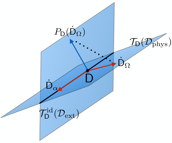
Section 4 discusses the identifiability problem in the stationary setting, see Figure 2. We define an equivalence relation between dynamical parameters for which the stationary output states are identical for all times $t$. In Theorem 1 we show that two dynamical parameters $\mathsf{D}$ and $\mathsf{D}^{\prime}$ are equivalent if and only if they are related by the “gauge transformation” $H^{\prime}=W^{*}HW+r\mathbbm{1}$ and $L^{\prime}_{i}=W^{*}L_{i}W$, where $W$ is unitary and $r$ is a real constant. From a differential geometry viewpoint, the space of identifiable parameters is the quotient $\mathcal{P}:=\mathcal{D}^{erg}/G$, where $\mathcal{D}^{erg}$ is the manifold of dynamical parameters $\mathsf{D}$ with ergodic dynamics, and $G=PU(d)\times\mathbb{R}$ is the group of “gauge transformations” whose orbits are the equivalence classes of parameters. In particular, we show that $\mathcal{D}^{erg}$ is a principal $G$-bundle over the base manifold $\mathcal{P}$. The vertical bundle over $\mathcal{D}^{erg}$ consists of subspaces $\mathcal{T}^{\rm nonid}_{\mathsf{D}}$ of the tangent space $\mathcal{T}_{\mathsf{D}}$ at $\mathsf{D}$, corresponding to un-identifiable changes of parameters, i.e. infinitesimal changes induced by the action of the group $G$. Although in general there is no canonical decomposition of the tangent space into “identifiable” and “non-indentifiable” components (i.e. $\mathcal{T}_{\mathsf{D}}=\mathcal{T}^{\rm nonid}_{\mathsf{D}}\oplus\mathcal{T}^{\rm id}_{\mathsf{D}}$), such a decomposition can be obtained from a principal connection, in a covariant way. A natural choice of connection is provided by the information geometry, as discussed below. This approach to system identification often appears in the classical setting, and the advantage is that one gains insight in the geometric structure of the parameter manifold, beyond the direct computation of the Fisher information. For instance, the connection can be useful for developing recursive estimation algorithms based on geodesics of the manifold [35]. For the standard theory of connections on principal bundles, see e.g. [38].

In Section 5 we derive the information geometric structure of the statistical estimation problem at hand. Before discussing the statistical aspects, we describe the basic elements of a theory of “output fluctuations” which is essential for information geometry, but has an interest in its own and deserves to be further investigated. For each $(k+1)$-tuple of system operators ${\bf X}=(X^{0},X^{1},\dots,X^{k})\in M(\mathbb{C}^{d})^{k+1}$ we define the associated fluctuation operator $\mathbb{F}_{t}({\bf X})$ given by the quantum stochastic integral

$$\mathbb{F}_{t}({\bf X})=\frac{1}{\sqrt{t}}\int_{0}^{t}\left(i\sum_{i=1}^{k}j_{s}(X^{i})dA^{*}_{i}(s)+j_{s}\circ\mathcal{C}_{\mathsf{D}}(X^{0})ds\right),\qquad\mathcal{C}_{\mathsf{D}}(X):=X-{\rm tr}[\rho^{ss}_{\mathsf{D}}X]\mathbbm{1},$$

where $j_{s}(X):=U_{\mathsf{D}}^{*}(s)XU_{\mathsf{D}}(s)$ is the time-evolved operator $X$. The covariance of $\mathbb{F}_{t}({\bf X})$ converges in the limit of large times, and defines a positive (but degenerate) inner product on $M(\mathbb{C}^{d})^{k+1}$ (cf. Proposition 1 for the explicit formula)

$$({\bf X},{\bf Y})_{\mathsf{D}}=\lim_{t\to\infty}\langle\mathbb{F}_{t}({\bf X})^{*}\mathbb{F}_{t}({\bf Y})\rangle.$$

Furthermore, in Propositions 1 and 2 we construct a linear map $R_{\mathsf{D}}:M(\mathbb{C}^{d})^{k+1}\to M(\mathbb{C}^{d})^{k+1}$ such that $R_{\mathsf{D}}$ is a projection onto the subspace of operators of the form $(0,Y^{1},\dots,Y^{k})\in M(\mathbb{C}^{d})^{k+1}$, and the kernel of $R_{\mathsf{D}}$ is the subspace of degenerate vectors of the inner product. With this definition, the inner product take the following simple form

$$({\bf X},{\bf Y})_{\mathsf{D}}=\sum_{i=1}^{k}{\rm tr}\left[\rho_{ss}R_{\mathsf{D}}({\bf X})^{i*}R_{\mathsf{D}}({\bf Y})^{i}\right].$$

We denote by $\dot{\mathsf{D}}=(\dot{H},\dot{L}^{1},\ldots,\dot{L}^{k})$ an element of the tangent space $\mathcal{T}_{\mathsf{D}}$. The real linear map ${\bf X}_{\mathsf{D}}$ defined below plays an important role in connecting fluctuation operators with the information geometry

	$\displaystyle{\bf X}_{\mathsf{D}}:\mathcal{T}_{\mathsf{D}}$	$\displaystyle\to$	$\displaystyle M(\mathbb{C}^{d})^{k+1}$
	$\displaystyle\dot{\mathsf{D}}$	$\displaystyle\mapsto$	$\displaystyle(\mathcal{E}_{\mathsf{D}}(\dot{\mathsf{D}}),\dot{L}^{1},\ldots,\dot{L}^{k})$

where $\mathcal{E}_{\mathsf{D}}$ is the map

	$\displaystyle\mathcal{E}_{\mathsf{D}}:\mathcal{T}_{\mathsf{D}}$	$\displaystyle\to$	$\displaystyle M(\mathbb{C}^{d})$
	$\displaystyle\mathcal{E}_{\mathsf{D}}:\dot{\mathsf{D}}$	$\displaystyle\mapsto$	$\displaystyle\dot{H}+\mathrm{Im}\sum_{i=1}^{k}\dot{L}^{i*}L^{i}.$

Here the second term in $\mathcal{E}_{\mathsf{D}}$ is due to quantum Ito calculus, hence in some sense represents the effects of the stochastic output on the information geometry. Using the map ${\bf X}_{\mathsf{D}}$ we define a real inner product on the tangent space $\mathcal{T}_{\mathsf{D}}$

$$(\dot{\mathsf{D}},\dot{\mathsf{D}}^{\prime})\longmapsto{\rm Re}({\bf X}_{\mathsf{D}}(\dot{\mathsf{D}}),{\bf X}_{\mathsf{D}}(\dot{\mathsf{D}}^{\prime}))_{\mathsf{D}}.$$

Moreover, since ${\bf X}_{\mathsf{D}}$ is injective, we can use it to define a projection $P_{\mathsf{D}}={\bf X}_{\mathsf{D}}^{-1}\circ R_{\mathsf{D}}\circ{\bf X}_{\mathsf{D}}$ acting on $\mathcal{T}_{\mathsf{D}}$. Its kernel is the vertical space $\mathcal{T}_{\mathsf{D}}^{\rm nonid}$ whose vectors correspond to infinitesimal “gauge transformations”, and are the degenerate vectors of the inner product. The range of $P_{\mathsf{D}}$ consists of tangent vectors satisfying the condition $\mathcal{E}_{\mathsf{D}}(\dot{\mathsf{D}})=0$. In particular, since $P_{\mathsf{D}}$ is a projection, the tangent space can be decomposed into “identifiable” and “non-identifiable” directions (see right panel of Figure 2)

$$\mathcal{T}_{\mathsf{D}}={\rm ran}P_{\mathsf{D}}\oplus{\rm ker}P_{\mathsf{D}}=\mathcal{T}_{\mathsf{D}}^{\rm id}\oplus\mathcal{T}_{\mathsf{D}}^{\rm nonid}$$

whose statistical interpretation is discussed below. This split has also an interesting differential geometric interpretation: the above tangent space decomposition, and inner product are covariant with respect to the action of the group $G$ and define a connection on the resulting principal $G$-bundle, with the associated Lie algebra valued one-form

$$\omega_{\mathsf{D}}:\mathcal{T}_{\mathsf{D}}\to\mathfrak{g},\quad\omega_{\mathsf{D}}(\dot{\mathsf{D}})=(\mathbb{W}_{\mathsf{D}}^{-1}\circ\mathcal{E}_{\mathsf{D}}^{0}(\dot{\mathsf{D}}),{\rm tr}[\rho_{ss}\mathcal{E}_{\mathsf{D}}(\dot{\mathsf{D}})])$$

explicitly depending on the map $\mathcal{E}_{\mathsf{D}}(\dot{\mathsf{D}})$ containing the essential quantum Ito correction. Moreover, the strictly positive inner product on $\mathcal{T}_{\mathsf{D}}^{\rm id}$ induces a strictly positive inner product on the tangent space $\mathcal{T}_{[\mathsf{D}]}$ to the point $[\mathsf{D}]$ in the base space $\mathcal{P}=\mathcal{D}^{erg}/G$ of identifiable parameters. As we will see below, this Riemannian metric is closely connected to the quantum Fisher information rate of the output state, so we will refer to it as the information geometry of the open quantum system, in analogy to the classical case [2].

Let us consider now the problem of estimating the dynamical parameter $\mathsf{D}$. Although the key constructions could be introduced in a “coordinate free” way, in order to emphasise the statistical aspects we choose to work with a given (but arbitrary) parametrisation $\theta\mapsto\mathsf{D}_{\theta}$ of $\mathcal{D}^{erg}$, where $\theta$ is an unknown parameter belonging to an open subset of $\mathbb{R}^{m}$, with $m:={\rm dim}(\mathcal{D}^{erg})$. At a given point $\mathsf{D}=\mathsf{D}_{\theta}\in\mathcal{D}^{erg}$, we define the tangent vectors $\dot{\mathsf{D}}_{a}:=\partial\mathsf{D}/\partial\theta_{a}=(\dot{H}_{a},\dot{L}^{1}_{a},\dots,\dot{L}^{k}_{a})$ describing infinitesimal changes of the coordinate $\theta_{a}$, for $a=1,\dots,m$; these vectors form a basis of the tangent space $\mathcal{T}_{\mathsf{D}}$.

We consider now the $m\times m$ quantum Fisher information (QFI) matrix $F^{\theta}(t)$ associated to the system-output state $|\Psi^{\rm s+o}_{\mathsf{D}_{\theta}}(t)\rangle$. The QFI is proportional to the real part of the covariance matrix of (centred) “generators” $G^{0}_{\theta,a}(t)$ of infinitesimal changes with respect to parameter component $\theta_{a}$ [11]. We show that the generator $G^{0}_{\theta,a}(t)$ (normalised by $t^{-1/2}$) can be expressed as a fluctuation operator $\mathbb{F}_{t}({\bf X}_{\mathsf{D}}(\dot{\mathsf{D}}_{a}))$, using the map ${\bf X}_{\mathsf{D}}$ defined above. As consequence, the QFI grows linearly in time, and the QFI rate per time unit $f^{\theta}=\lim_{t\to\infty}F^{\theta}(t)/t$ can be expressed in terms of the Markov covariance as

	$\displaystyle f^{\theta}_{a,b}$	$\displaystyle=$	$\displaystyle 4{\rm Re}({\bf X}_{\mathsf{D}}(\dot{\mathsf{D}}_{a}),{\bf X}_{\mathsf{D}}(\dot{\mathsf{D}}_{b}))_{\mathsf{D}}=4{\rm Re}(R_{\mathsf{D}}{\bf X}_{\mathsf{D}}(\dot{\mathsf{D}}_{a}),R_{\mathsf{D}}{\bf X}_{\mathsf{D}}(\dot{\mathsf{D}}_{b}))_{\mathsf{D}}$
		$\displaystyle=$	$\displaystyle 4\sum_{i=1}^{k}{\rm Re}\,\mathrm{tr}\left[\rho_{ss}^{\mathsf{D}}\left(\dot{L}^{i}_{a}-i[L^{i},\mathbb{W}_{\mathsf{D}}^{-1}\circ\mathcal{E}^{0}_{\mathsf{D}}(\dot{\mathsf{D}}_{a})]\right)^{*}\cdot\left(\dot{L}^{i}_{b}-i[L^{i},\mathbb{W}_{\mathsf{D}}^{-1}\circ\mathcal{E}^{0}_{\mathsf{D}}(\dot{\mathsf{D}}_{b})]\right)\right].$

where $\mathbb{W}_{\mathsf{D}}$ is the Lindblad operator at $\mathsf{D}$. In particular, the Fisher information rate associated to directions in vertical bundle $\mathcal{T}_{\mathsf{D}}^{\rm nonid}$ (gauge transformations) is equal to zero as expected from the invariance of the output state. This follows from the fact that ${\bf X}_{\mathsf{D}}$ maps $\mathcal{T}_{\mathsf{D}}^{\rm nonid}$ into ${\rm ker}R_{D}$.

Above we saw that the real part of the Markov covariance $(\cdot,\cdot)_{\mathsf{D}}$ defines a positive definite inner product on the real space $\mathcal{T}^{\rm id}_{\mathsf{D}}$. In fact, $\mathcal{T}^{\rm id}_{\mathsf{D}}$ can be made into a complex space by introducing the complex structure

	$\displaystyle\mathcal{J}_{\mathsf{D}}:\mathcal{T}^{id}_{\mathsf{D}}$	$\displaystyle\to$	$\displaystyle\mathcal{T}^{id}_{\mathsf{D}}$
(1)		$\displaystyle\mathcal{J}_{\mathsf{D}}:(\dot{H},\dot{L}^{1},\ldots,\dot{L}^{k})$	$\displaystyle\mapsto$	$\displaystyle\left(\sum_{i=1}^{k}{\rm Re}\dot{L}^{i*}L^{i}\,,\,i\dot{L}^{1},\ldots,i\dot{L}^{k}\right).$

With this definition the map ${\bf X}_{\mathsf{D}}$ becomes an isomorphism of complex spaces and $(\cdot,\cdot)_{\mathsf{D}}$ defines a complex inner product on $(\mathcal{T}^{\rm id}_{\mathsf{D}},\mathcal{J}_{\mathsf{D}})$. Using the imaginary part $\sigma_{D}$ of the inner product, we define the canonical commutation relations (CCR) algebra $CCR(\mathcal{T}_{\mathsf{D}}^{\rm id},\sigma^{\mathsf{D}})$ generated by Weyl operators with commutation relations

$$W(\dot{\mathsf{D}})W(\dot{\mathsf{D}}^{\prime})=e^{i\sigma^{\mathsf{D}}(\dot{\mathsf{D}},\dot{\mathsf{D}}^{\prime})}W(\dot{\mathsf{D}}+\dot{\mathsf{D}}^{\prime}),\quad W(-\dot{\mathsf{D}})=W(\dot{\mathsf{D}})^{*},\quad\dot{\mathsf{D}},\dot{\mathsf{D}}^{\prime}\in\mathcal{T}^{\rm id}_{\mathsf{D}}.$$

Following a standard construction we define the Fock representation and the coherent states $|\dot{\mathsf{D}}\rangle:=W(\dot{\mathsf{D}})|0\rangle$, where $|0\rangle$ is the vacuum state $\langle 0|W(\dot{\mathsf{D}})|0\rangle=\exp(-(\dot{\mathsf{D}},\dot{\mathsf{D}})_{\mathsf{D}}/2)$ This model will be interpreted below as limit of the output state model for large times.

Section 6 details the above constructions in the case of special one dimensional models, and for a general multidimensional model for a two dimensional system.

In section 7 we study the asymptotic statistical structure of the output state. The main result is the local asymptotic normality (LAN) Theorem 2 which shows that both the system-output state, and the stationary output state can be approximated by coherent states of the CCR algebra $CCR(\mathcal{T}_{\mathsf{D}}^{\rm id},\sigma_{\mathsf{D}})$. Below we give a brief description of the result and its interpretation.

Let us consider a parametrisation $u\mapsto[\mathsf{D}]_{u}$ of (an open subset of) the space of identifiable parameters $\mathcal{P}=\mathcal{D}^{erg}/G$, such that the origin $u=0$ corresponds to a given parameter of interest $[\mathsf{D}_{0}]=[\mathsf{D}]_{u=0}$. We define the time-indexed family of “local” statistical models

$$\tilde{\mathcal{Q}}_{t}:=\left\{\rho^{\rm out}_{u/\sqrt{t}}(t):u\in\mathcal{O}\subset\mathbb{R}^{{\rm dim}(\mathcal{P})}\right\}$$

which consist of the output state for unknown parameter values $u/\sqrt{t}$ in a shrinking ball of size scaling as the statistical uncertainty. The local model $\tilde{\mathcal{Q}}_{t}$ captures the asymptotic properties of the quantum output state for parameters in a neighbourhood of $[\mathsf{D}_{0}]$, and it can be justified operationally by means of adaptive procedures whereby a “small part” of the output can be used to localise the parameter, while the “remaining part” can be used for estimating the local parameter $u$ (cf. [30] for a similar argument in the state estimation setup).

To define the system-output statistical model let us consider a horisontal section $s:\mathcal{P}\to\mathcal{D}^{erg}$ of the principal bundle, i.e. the tangent space to $s(\mathcal{P})$ at $\mathsf{D}$ is the horisontal space $\mathcal{T}_{\mathsf{D}}^{id}$. Let

$$\mathcal{Q}_{t}:=\left\{\left|\Psi^{\rm s+o}_{u/\sqrt{t}}(t)\right\rangle:u\in\mathcal{O}\subset\mathbb{R}^{{\rm dim}(\mathcal{P})}\right\},$$

be the quantum statistical model where $\left|\Psi^{\rm s+o}_{u/\sqrt{t}}(t)\right\rangle$ is the joint system-output state at time $t$ at the dynamical parameter $\mathsf{D}_{u}=s([D]_{u})$. The reasons for using a horisontal section in defining the model are as follows. While the stationary output state depends only on the identifiable parameters in $\mathcal{P}$, the system-output state is also sensitive to the location of the parameter within an orbit. It turns out that the asymptotic properties can be captured most transparently by choosing a horisontal section which sets certain unphysical phase factors to zero and allows us to understand the model directly in terms of the geometric properties of the vector state, as explained below.

Finally, we define the Gaussian model

$$\mathcal{G}:=\left\{\rho_{u}:=|u\rangle\langle u|:u\in\mathcal{O}\subset\mathbb{R}^{{\rm dim}(\mathcal{P})}\right\}$$

where $|u\rangle=W(\sum_{a}u_{a}\dot{\mathsf{D}}_{a})|0\rangle$ is the coherent state of the CCR algebra $CCR(\mathcal{T}^{id}_{\mathsf{D}_{0}},\sigma^{\mathsf{D}_{0}})$. By construction, the QFI of this model is equal to the QFI rate $f$ of the output state at $[\mathsf{D}_{0}]$, which also the QFI of the output state with respect to the local parameter $u$, rather than the “true” parameter $u/\sqrt{t}$.

The first version of LAN states that $\mathcal{Q}_{t}$ converges (weakly) to $\mathcal{G}$ for large times in the sense of convergence of the inner products (uniformly in $u,v\in\mathcal{O}$), as illustrated in Figure 3

$$\lim_{n\to\infty}\left\langle\Psi^{\rm s+o}_{u/\sqrt{t}}(t)\right|\left.\Psi^{\rm s+o}_{v/\sqrt{t}}(t)\right\rangle=\langle u|v\rangle.$$

Since pure state models are fully characterised by the inner products, the convergence simply means that for large times the geometry of the system-output states is very similar to that of the coherent states. Although intuitive, this notion of convergence is not suitable for mixed states such as that of the output, and does not have a direct operational meaning. In the second version of LAN we show that the output models $\tilde{\mathcal{Q}}_{t}$ converge strongly to $\mathcal{G}$ in the sense that there exist channels $T_{t}$ and $S_{t}$ such that

	$\displaystyle\lim_{t\to\infty}\sup_{u\in\mathcal{O}}\left\|T_{t}\left(\rho^{\rm out}_{u/\sqrt{t}}(t)\right)-\rho_{u}\right\|_{1}=0$
	$\displaystyle\lim_{t\to\infty}\sup_{u\in\mathcal{O}}\left\|S_{t}\left(\rho_{u}\right)-\rho^{\rm out}_{u/\sqrt{t}}(t)\right\|_{1}=0.$

A concrete consequence of this “convergence to Gaussianity” is that the QFI computed above is asymptotically “achievable” in the sense that the estimation of dynamical parameters reduces to that of estimating a Gaussian displacement family with QFI equal to $f_{a,b}$. Similarly to LAN for ensembles of identical states [30], the result implies that the optimal measurement is a linear one (i.e. of homodyne and heterodyne type) and the errors are normally distributed. However, since this paper concentrates on the structure of the quantum states, the measurement and estimation procedures are not discussed here.

We begin by introducing notations and necessary background about the input-output formalism of continuous-time quantum Markov processes [23]. The formalism describes the joint unitary evolution of an open quantum system interacting with a Bosonic environment in the Markov regime, cf. Figure 1. From this, one can derive the reduced (master) dynamics of the system, as well as the stochastic Schrödinger equations for quantum trajectories, describing the stochastic evolution of the system conditional on observations produced by a continuous-time measurement on the environment. However, in this paper we will be mainly interested in the output quantum state, i.e. the state of the environment after the interaction with the system.

Throughout the paper we assume the system to be finite-dimensional, with Hilbert space $\mathcal{H}=\mathbb{C}^{d}$, and associated algebra of observables $\mathcal{A}=M(\mathbb{C}^{d})$. As we will detail below, the dynamics is specified by the system Hamiltonian $H$, together with the quantum jump operators $L^{1},\dots,L^{k}$. We denote these collectively by

$$\mathsf{D}=(H,L^{1},\ldots,L^{k})=(H,{\bf L})\in\mathcal{D}:=M_{sa}(\mathbb{C}^{d})\times M(\mathbb{C}^{d})^{k},$$

and refer to each $\mathsf{D}\in\mathcal{D}$ as a dynamical parameter, and to $\mathcal{D}$ as manifold (space) of dynamical parameters.

This section deals with the problem of characterising the equivalence classes of Markov dynamics with identical stationary output states. We restrict ourselves to ergodic Markov processes, although similar results are expected to hold more generally. Similar results have been obtained in [31] for discrete time quantum Markov processes.

Let $\mathcal{D}^{\rm erg}$ denote the open subset of $\mathcal{D}$ consisting of dynamical parameters for which the associated Markov process is ergodic; this will be the relevant paramter set for subsequent considerations.

Of course, the same equivalence can be formulated for arbitrary parameters in $\mathcal{D}$. However, it turns out that when restricted to $\mathcal{D}^{\rm erg}$, the equivalence classes have a simple characterisation in terms of the following transformations:

• (PM)

  Phase conjugation on the Hamiltonian:

  $$(H,L^{1},\ldots,L^{k})\mapsto(H+r\mathbbm{1},L^{1},\ldots,L^{k}),\quad(r\in\mathbb{R}).$$

• (UC)

  Conjugation by system unitary $W$:

  $$(H,L^{1},\ldots,L^{k})\mapsto(W^{*}HW,W^{*}L^{1}W,\ldots,W^{*}L^{k}W).$$

Indeed, it is easy to verify that (PM) and (UC) do not change the output of the associated continuous Markov process. The following Theorem shows that the converse is also true. The details of the proof can be found in Appendix 8.

The interpretation of the result is that parameters along the equivalence classes described by the transformations (UC) and (PM) are not identifiable, while the identifiable parameters are “transversal” to these classes, as illustrated in Figure 2. It is now convenient to formulate the equivalence classes in terms of an action of the appropriate Lie group $G:=PU(d)\times\mathbb{R}$. For that we regard $\mathcal{D}^{\rm erg}$ as an open submanifold of $\mathcal{D}$, and use transformations (PM) and (UC) to set up the action:

		$\displaystyle G\times\mathcal{D}^{\rm erg}\to\mathcal{D}^{\rm erg}$
(10)			$\displaystyle(g,\mathsf{D})\mapsto g\mathsf{D}:=(W^{*}HW,W^{*}L^{1}W,\ldots,W^{*}L^{k}W)+a(\mathbbm{1},0,\ldots,0),$
		$\displaystyle g=(W,a)\in PU(d)\times\mathbb{R},\quad\mathsf{D}=(H,L^{1},\ldots,L^{k})\in\mathcal{D}^{\rm erg}.$

Here $PU(d)=U(d)/U(1)$ is the projective unitary group, equipped with its unique Lie group structure, and the above action is defined as the natural lift of the corresponding one for $U(d)$. The reason to use $PU(d)$ instead of $U(d)$ will become clear from the proof of the Lemma below.

The above theorem implies that the equivalence class $[\mathsf{D}]\in\mathcal{P}$ is the orbit of $D\in\mathcal{D}^{\rm erg}$ under the action of $G$, such that $\mathcal{P}$ can be identified with the quotient $\mathcal{D}^{\rm erg}/G$. The following lemma which relies on the ergodicity assumption, is essential for understanding the structure of the quotient, as we will see below. In order to avoid confusion with the output equivalence, we identify $W\in PU(d)$ with a representative unitary operator without explicit indication.

The fact that the group action preserves the equivalence classes, that is $g\mathsf{D}\in[\mathsf{D}]$ for all $\mathsf{D}\in\mathcal{D}^{\rm erg}$, can now be formulated in differential geometric terms. Indeed, using the standard theory of Lie group actions on manifolds, we conclude from the above Lemma that the space of output equivalence classes

$$\mathcal{P}=\{[\mathsf{D}]~:~\mathsf{D}\in\mathcal{D}^{\rm erg}\}=\mathcal{D}^{\rm erg}/G$$

admits a unique smooth structure such that the quotient map $\pi:\mathcal{D}^{\rm erg}\to\mathcal{P}$

$$\pi(\mathsf{D})=[\mathsf{D}],\quad\text{ for all }\mathsf{D}\in\mathcal{D}^{\rm erg},$$

is a submersion, and $\mathcal{D}^{\rm erg}$ is a principal $G$-bundle over $\mathcal{P}$ [38]. Here the equivalence classes $[\mathsf{D}]$ are considered as fibres of the fiber bundle over the base manifold $\mathcal{P}$, that is, the map $\pi$ has the local triviality property: each $[D]\in\mathcal{P}$ has an open neighbourhood $U$ such that there exists a diffeomorphism

$$\phi:\pi^{-1}(U)\to U\times G,$$

which is $G$-equivariant, i.e. $\phi(g\mathsf{D})=g\phi(\mathsf{D})$ where $G$ acts on $U\times G$ as $g([\mathsf{D}],g^{\prime}):=([\mathsf{D}],g^{\prime}g^{-1})$. The term principal $G$-bundle refers to the fact that the group action preserves the fibres.

We can now use this differential geometric framework to describe local changes of identifiable parameters, via the tangent bundle $\mathcal{T}$ of the manifold $\mathcal{D}^{\rm erg}$. In particular, the non-identifiable parameter changes along the equivalence classes correspond to the vertical bundle over $\mathcal{D}^{\rm erg}$ with the fibres

$$\mathcal{T}_{\mathsf{D}}^{\rm nonid}:=\ker\left.\pi_{*}\right|_{\mathsf{D}}\subset\mathcal{T}_{\mathsf{D}},\quad\mathsf{D}\in\mathcal{D}^{\rm erg},$$

where $\left.\pi_{*}\right|_{\mathsf{D}}$ is the push-forward tangent map of the canonical projection $\pi$ at point $\mathsf{D}$, and $\mathcal{T}_{\mathsf{D}}$ is the full tangent space at that point.

The group action is reflected in two ways at the level of tangent spaces. On the one hand, given any fixed $g\in G$, the push-forward $g_{*}$ of the map $\mathsf{D}\mapsto g\mathsf{D}$ maps the fibres into each other as

$$g_{*}\mathcal{T}^{\rm nonid}_{\mathsf{D}}=\mathcal{T}^{\rm nonid}_{g\mathsf{D}}.$$

This push-forward is simply obtained by differentiating the parameters in the standard chart

$$g_{*}(\dot{H},\dot{L}^{1},\ldots,\dot{L}^{k})=(W^{*}\dot{H}W,W^{*}\dot{L}^{1}W,\ldots,W^{*}\dot{L}^{k}W),\quad g=(W,a).$$

On the other hand, for any fixed $\mathsf{D}$, the push-forward of $g\mapsto g\mathsf{D}$ defines a Lie algebra isomorphism

(11)

$$\mathsf{D}_{*}:\mathfrak{g}\to\mathcal{T}^{\rm nonid}_{\mathsf{D}},$$

so that different fibres all have the same dimension, which is that of the Lie algebra $\mathfrak{g}$. We can now explicitly compute this action. First of all, the Lie algebra of $G$ can be conveniently written as

(12)

$$\mathfrak{g}=\{(-iK,r)\mid K\in M_{sa}(\mathbb{C}^{d})/\mathbb{R}\mathbbm{1},\,r\in\mathbb{R}\}=\{(-iK,r)\mid K\in M_{sa}(\mathbb{C}^{d}),\,{\rm tr}[\rho^{ss}K]=0,\,r\in\mathbb{R}\},$$

where the choice of the sign as well as the last identification is for later convenience. In particular, the subspace of non-identifiable directions is in one-to-one correspondence with this linear space. From this we already find the number of non-identifiable directions:

$$\dim\mathcal{T}^{\rm nonid}_{\mathsf{D}}=d^{2}-1+1=d^{2}.$$

We stress that this result is crucially based on ergodicity, which ensures that the action is free; this is required for the push-forward $\mathsf{D}_{*}$ to be an isomorphism. Now $\mathsf{D}_{*}$ acts on an element $X=(-iK,r)\in\mathfrak{g}$ as

	$\displaystyle\mathsf{D}_{*}(X)$	$\displaystyle=\frac{d}{dt}(\exp(t\,(-iK,r))\mathsf{D})|_{t=0}$
		$\displaystyle=\frac{d}{dt}\left((e^{itK}He^{-itK},e^{itK}L^{1}e^{-itK},\ldots,e^{itK}L^{k}e^{-itK})+t\,r(\mathbbm{1},0,\ldots,0)\right)|_{t=0}$
		$\displaystyle=(i[H,K],i[L^{1},K],\ldots,i[L^{k},K])+r(\mathbbm{1},0,\ldots,0).$

Having now characterised the vertical bundle $\mathcal{T}^{\rm nonid}$ of non-identifiable directions, an obvious question arises: is there a natural way to choose complementary subspaces for identifiable directions in each fibre? This means choosing subspaces $\mathcal{T}^{\rm id}_{\mathsf{D}}$ such that

$$\mathcal{T}_{\mathsf{D}}=\mathcal{T}^{\rm nonid}_{\mathsf{D}}\oplus\mathcal{T}^{\rm id}_{\mathsf{D}},\quad\mathsf{D}\in\mathcal{D}^{\rm erg}.$$

If the subspaces are chosen smoothly, i.e. so as to define a fibre bundle $\mathcal{T}^{\rm id}$ over $\mathcal{D}^{\rm erg}$, the result is called a horizontal bundle $\mathcal{T}^{\rm id}$, and in case it respects the group action, that is

(13)

$$g_{*}\mathcal{T}^{\rm id}_{\mathsf{D}}=\mathcal{T}^{\rm id}_{g\mathsf{D}},$$

it defines an principal connection on the manifold $\mathcal{D}^{\rm erg}$.

There is a natural way of defining a principal connection via its associated connection one-form; since this approach turns out to be relevant in our situation, we briefly explain the idea in the general level. As we have shown above, any $\dot{\mathsf{D}}\in\mathcal{T}^{\rm nonid}_{\mathsf{D}}$ can be generated by the action of the Lie algebra; $\dot{\mathsf{D}}=\mathsf{D}_{*}(X)$ for some $X\in\mathfrak{g}$. Now suppose that we can associate to every tangent vector $\dot{\mathsf{D}}\in\mathcal{T}_{\mathsf{D}}$ an element $\omega_{\mathsf{D}}(\dot{\mathsf{D}})\in\mathfrak{g}$ which somehow describes the ”part” of the parameter that results from the non-identifiable group action. Such a map should define a one-form $\omega:\mathcal{T}\to\mathfrak{g}$ satisfying the compatibility condition (sometimes called nondegeneracy)

(14)

$$\dot{\mathsf{D}}=\mathsf{D}_{*}(\omega_{\mathsf{D}}(\dot{\mathsf{D}})),\quad\dot{\mathsf{D}}\in\mathcal{T}^{\rm nonid}_{\mathsf{D}},$$

and the $G$-covariance condition

(15)

$$g^{*}\omega={\rm Ad}_{g^{-1}}\circ\omega,$$

where $g^{*}$ is the pull-back of the action by $g$ on the cotangent bundle, which simply acts as $g^{*}\omega(\dot{\mathsf{D}})=\omega_{g\mathsf{D}}(g_{*}\dot{\mathsf{D}})=\omega_{g\mathsf{D}}(W^{*}\dot{\mathsf{D}}W)$ for $g=(W,a)$, and the adjoint action is given by ${\rm Ad}_{g^{-1}}(X)=(W^{*}XW,r+a)$.

Given such a map, we can then define the ”back-action” $\mathsf{D}_{*}\circ\omega_{\mathsf{D}}$ on the tangent space; due to the above compatibility condition, the back-action is a special projection of the tangent space onto the subspace $\mathcal{T}^{\rm nonid}_{\mathsf{D}}$. Hence, we can use its complementary projection

$$P_{\mathsf{D}}:={\rm Id}-\mathsf{D}_{*}\circ\omega_{\mathsf{D}}$$

to define the above horizontal bundle and the associated principal connection via

$$\mathcal{T}^{\rm id}_{\mathsf{D}}:={\rm ran}\,P_{\mathsf{D}}.$$

Indeed, the condition (13) holds because of (15). The map $\omega$ is called the connection one-form, and $P_{\mathsf{D}}$ is the horizontal projection.

Any principal connection gives a possible way of extracting the parameter changes relevant for our system identification problem. In the next section we show that there is actually a natural connection associated with the information geometric structure of the problem, given by the Fisher information of the output state. We will obtain it by explicitly constructing the associated connection one-form, which arises neatly from the quantum Ito calculus.

Our goal is to describe quantitatively the precision with which unknown dynamical parameters can be estimated by making measurements on the output state. As noted above, we will restrict our attention to dynamical parameters $\mathsf{D}$ which belong to the open subset $\mathcal{D}^{\rm erg}$ of $\mathcal{D}$ of ergodic Markov dynamics. As we will consider this problem in the limit of large times, the relevant dynamical regime is the stationary one; moreover, the statistical properties of the output state can be understood locally, by focusing on a shrinking neighbourhood of the parameter manifold $\mathcal{D}^{\rm erg}$ whose size is of the order of the statistical uncertainty [31, 13]. This will lead to the concept of local asymptotic normality discussed in section 7. In this section however, we focus on the information geometry of the system identification problem, more precisely on the quantum Fisher information matrix of the output state and its asymptotic behaviour, and its relationship with the covariance of certain quanta stochastic integrals called “fluctuation operators”. We will start by introducing the latter in a general set-up and then show how the former fits in this theory.

Section 5.1 derives the quantum Fisher information of the system-output state as covariance of certain “generators”; section 5.2 analyses more general “fluctuation operators” and looks at their Markov covariance; section 5.3 deals with the information geometry structure, and connects the previous constructions, in particular it provides an explicit expression of the quantum Fisher information; section 5.4 constructs an algebra of canonical commutation relations (multimode continuous variables system) and a family of coherent states which will be relevant later on for the local asymptotic result.

References

- [1] V. V. Albert, B. Bradlyn, M. Fraas, and L. Jiang. Geometry and response of Lindbladians. arXiv:1512.08079.
- [2] S. Amari and H. Nagaoka. Methods of Information Geometry, volume 191 of Translations of mathematical monographs. American Mathematical Society, 2000.
- [3] J.E. Avron, M. Fraas, and G.M. Graf. Adiabatic response for lindblad dynamics. J. Stat. Phys., 148:800–823, 2012.
- [4] L. Banchi, P. Giorda, and P. Zanardi. Quantum information-geometry of dissipative quantum phase transitions. Phys. Rev. A, 89:022102, 2014.
- [5] B. Baumgartner and H. Narnhofer. Analysis of quantum semigroups with GKSÐLindblad generators: II. General. J. Phys. A: Math. Theor., 41:395303, 2008.
- [6] T. Baumgratz, D. Gross, M. Cramer, and M.B. Plenio. Scalable reconstruction of density matrices. Phys. Rev. Lett., 111:020401, 2013.
- [7] V. P. Belavkin. Quantum stochastic calculus and quantum nonlinear filtering. J. Multivar. Anal., 42:171–201, 1992.
- [8] V. P. Belavkin. Measurement, filtering and control in quantum open dynamical systems. Rep. Math. Phys., 43:405–425, 1999.
- [9] P.J. Bickel, Y. Ritov, and T. Ryden. Inference in hidden Markov models I: Local asymptotic normality in the stationary case. Bernoulli, 2:199–291, 1996.
- [10] L. Bouten, R. van Handel, and M. James. An introduction to quantum filtering. SIAM J. Control Optim., 46:2199–2241, 2007.
- [11] Samuel L. Braunstein and Carlton M. Caves. Statistical distance and the geometry of quantum states. Phys. Rev. Lett., 72:3439–3443, 1994.
- [12] H-P. Breuer and F. Petruccione. The theory of open quantum systems. Oxford University Pressl, 2002.
- [13] C. Catana, M. Guţă, and L. Bouten. Fisher informations and local asymptotic normality for continuous-time quantum Markov processes. J. Phys. A, 48:365301, 2015.
- [14] C. Catana, M. Guţă, and T. Kypraios. Maximum likelihood versus likelihood-free quantum system identification in the atom maser. arXiv:1311.4091, to appear in J. Phys. A, 2013.
- [15] A. Chefles, R. Josza, and A. Winter. On the existence of physical transformations between sets of quantum states. Int. J. Quantum Inform., 02:11, 2004.
- [16] M Cozzini, R. Ionicioiu, and P. Zanardi. Quantum fidelity and quantum phase transitions in matrix product states. Phys. Rev. B, 76:104420, 2007.
- [17] D.G. Evans, J. E. Gough, and M. R. James. Non-abelian weyl commutation relations and the series product of quantum stochastic evolutions. Phil. Trans. R. Soc. A, 370:5437–5451, 2012.
- [18] M. Fannes, B. Nachtergaele, and R. F. Werner. Finitely correlated states on quantum spin chains. Commun. Math. Phys., 144:443, 1992.
- [19] A. Frigerio. Stationary states of quantum dynamical semigroups. Comm. Math. Phys., 63:269–276, 1978.
- [20] J. Gambetta and H.M. Wiseman. State and dynamical parameter estimation for open quantum systems. Phys.Rev. A, 64:042105, 2001.
- [21] S. Gammelmark and K. Molmer. Bayesian parameter inference from continuously monitored quantum systems. Phys. Rev. A, 87:032115, 2013.
- [22] Søren Gammelmark and Klaus Mølmer. Fisher Information and the Quantum Cramér-Rao Sensitivity Limit of Continuous Measurements. Phys. Rev. Lett., 112:170401, 2014.
- [23] C. Gardiner and P. Zoller. Quantum Noise. Springer, 2004.
- [24] R. D. Gill and M. Guţă. On Asymptotic Quantum Statistical Inference. Institute of Mathematical Statistics Collections, 9:105–127, 2012.
- [25] J. Gough and M.R. James. The series product and its application to quantum feedforward and feedback networks. IEEE Transactions on Automatic Control, 54:2530–2544, 2009.
- [26] J. E. Gough, T. S. Ratiu, and O. G. Smolyanov. NoetherÕs theorem for dissipative quantum dynamical semi-groups. J. Math. Phys, 56:022108, 2015.
- [27] M. Guţă. Quantum Fisher information and asymptotic normality in system identification for quantum Markov chains. Phys. Rev . A, 83:062624, 2011.
- [28] M. Guţă, B. Janssens, and J. Kahn. Optimal estimation of qubit states with continuous time measurements. Commun. Math. Phys., 277:127–160, 2008.
- [29] M. Guţă and A. Jençová. Local asymptotic normality in quantum statistics. Commun. Math. Phys., 276:341–379, 2007.
- [30] M. Guţă and J. Kahn. Local asymptotic normality for qubit states. Phys. Rev. A, 73:052108, 2006.
- [31] M. Guţă and J. Kiukas. Equivalence Classes and Local Asymptotic Normality in System Identification for Quantum Markov Chains. Commun. Math. Phys., 335:1397–1428, 2015.
- [32] M. Guţă and N. Yamamoto. System Identification for Passive Linear Quantum Systems. arXiv:1303.3771v2, to appear in IEEE Transactions on Automatic Control 2016.
- [33] J. Haegeman, M. Marien, T.J. Osborne, and F. Verstraete. Geometry of matrix product states: metric, parallel transport and curvature. J. Math. Phys., 55:021902, 2014.
- [34] Jutho Haegeman, Tobias J. Osborne, and Frank Verstraete. Post-matrix product state methods: To tangent space and beyond. Phys. Rev. B, 88:075133, Aug 2013.
- [35] B. Hanzon. On a coordinate free prediction error algorithm for system identification. In C.I. Byrnes and A. Lindquist, editors, Modelling, Identification and Robust Control, page 595. Elsevier Science Publishers B.V., 1986.
- [36] A. Holevo. Probabilistic and Statistical Aspects of Quantum Theory. North-Holland Publishing Company, Amsterdam-New York-Oxford, 1982.
- [37] R. Höpfner, J. Jacod, and L. Ladelli. Local asymptotic normality and mixed normality for markov statistical models. Prob. Theory Rel. Fields, 86:105–129, 1990.
- [38] C.J. Isham. Modern Differential Geometry for Physicists, 2nd Ed. World Scientific, 2003.
- [39] M.R. James, H.I. Nurdin, and I.R. Petersen. H-infinity control of linear quantum stochastic systems. IEEE Transactions on Automatic Control, 53:1787–1803, 2008.
- [40] J. Kahn and M. Guţă. Local asymptotic normality for finite dimensional quantum systems. Commun. Math. Phys., 289:597–652, 2009.
- [41] L. Le Cam. Asymptotic Methods in Statistical Decision Theory. Springer Verlag, New York, 1986.
- [42] L. Ljung. System Identification Theory for the User. Prentice Hall, 1999.
- [43] H. Mabuchi. Dynamical identification of open quantum systems. Quantum Semiclass. Opt., 8:1103–1108, 1996.
- [44] K. Macieszczak, M. Guţă, I. Lesanovsky, and J.P. Garrahan. Dynamical phase transitions as a resource for quantum enhanced metrology. arXiv:1411.3914, to appear in Phys. Rev. A.
- [45] K. Macieszczak, M. Guţă, I. Lesanovsky, and J.P. Garrahan. Towards a theory of metastability in open quantum dynamics. arXiv:1512.05801.
- [46] K. R. Parthasarathy. An Introduction to Quantum Stochastic Calculus. Birkhäuser, Basel, 1992.
- [47] D. Petz. An Invitation to the Algebra of Canonical Commutation Relations. Leuven University Press, Leuven, 1990.
- [48] D. Petz and Jencova, A. Sufficiency in quantum statistical inference. Commun. Math. Phys., 263:259 – 276, 2006.
- [49] J. M. Radcliffe. Some properties of coherent spin states. J. Phys. A, 4:313–323, 1971.
- [50] David A. Sivak and Gavin E. Crooks. Thermodynamic metrics and optimal paths. Phys. Rev. Lett., 108:190602, May 2012.
- [51] M. M. Taddei, B. M. Escher, L. Davidovich, and R. L. de Matos Filho. Quantum speed limit for physical processes. Phys. Rev. Lett., 110:050402, 2013.
- [52] F. Verstraete and J. I. Cirac. Continuous matrix product states for quantum fields. Phys. Rev. Lett., 104:190405, 2010.
- [53] H. M. Wiseman and G. J. Milburn. Quantum Measurement and Control. Cambridge University Press, 2009.