跳到论文正文
W Papers独立论文阅读器 arXiv:1601.03962 论文正文 计算阅读时间 · 0%
引用这篇论文根据当前论文元数据生成,正式投稿前建议核对。


License: arXiv.org perpetual non-exclusive license
arXiv:1601.03962v3 [math.OC] 12 Jan 2017

Timing Options for a Startup with Early Termination and Competition Risks

Tim Leung ††thanks: Department of Applied Mathematics, University of Washington, Seattle, WA 98195. E-mail: timleung@uw.edu. Corresponding author.    Zongxi Li ††thanks: Operations Research & Financial Engineering Department, Princeton University, Princeton, NJ 08544. E-mail: zongxil@princeton.edu.
August 24, 2026
Abstract

This paper analyzes the timing options embedded in a startup firm, and the associated market entry and exit timing decisions under the exogenous risks of early termination and competitor’s entry. Our valuation approach leads to the analytical study of a non-standard perpetual American installment option nested with an optimal sequential stopping problem. Explicit formulas are derived for the firm’s value functions. Analytically and numerically, we show that early termination risk leads to earlier voluntary entry or exit, and the threat of competition has a non-trivial effect on the firm’s entry and abandonment strategies.

Keywords:  startup, market entry, project abandonment, early termination, competition risk

JEL Classification:  C41, G11, G13, M13

Mathematics Subject Classification (2010):  60G40, 62L15, 91G20, 91G80

1 Introduction

Over the past two decades, there have been a number of highly successful startup companies. Nevertheless, in general firms in their early stages require significant capital investment for research and development (R&D) and face tremendous amount risk that may force them to abandon the projects. Many startups may fail before they even sell a single unit of products. The risk of early termination may be due to demand uncertainty, technological challenges, regulatory changes, and other causes.

Another major risk factor for a startup is the emergence of a competitor. This is commonly seen in markets with very few major players, for example, Lyft’s entry to New York City to compete with Uber,11 1 http://www.wsj.com/articles/lyft-revs-up-in-new-york-city-1448038672 and the launch of Apple music to rival Pandora and Spotify.22 2 http://www.wsj.com/articles/apple-to-announce-new-music-services-1433183201 In effect, new competition may reduce the existing firm’s market share and thus revenue stream, as noted by Petersen and Bason (2001). In turn, this influences how long the firm can stay in the market.

In this paper, we propose a theoretical real option approach to better understand a startup firm’s strategies to voluntarily abandon a project or enter the market in face of early termination and competition risks. The arrivals of early termination and competition are modeled by exogenous independent exponential random variables. We analyze their combined impact on the firm’s optimal timing to enter or exit. Our valuation approach is a non-standard perpetual American installment option nested with an optimal sequential stopping problem.

Our main results are the analytic solutions for the firm’s sequential timing problems. We also investigate the impact of the early termination risk and the competitor’s potential entry on the firm’s value and the associated timing to enter and exit the market. Among our findings, the firm has a lower entry threshold and higher cancellation threshold when the early termination risk rises. On the other hand, competition risk may increase or decrease the firm’s abandonment level, depending on the impact on the new cash flow. We provide the necessary and sufficient condition for both cases. Numerical results are provided to illustrate these effects.

In the literature, Pennings and Lint (1997) study the empirical option value of an R&D project, and model the arrivals of new information that impact cash flows by exponential random variables. Lukas et al. (2016) propose an entrepreneurial venture financing model without competition risk by combining compound option pricing with sequential non-cooperative contracting. Kort and Wrzaczek (2015) apply a game-theoretic approach to study the incumbent’s over or under investment problem accounting for the threat of entry. Also, Restrepo et al. (2015) study a real option approach for sequential investments in the presence of expropriation risk. Davis et al. (2004) study the valuation of a venture capital as an installment option, while Ciurlia and Caperdoni (2009) and Kimura (2009) study the pricing of American installment put and call options. Our model can be viewed as a perpetual American-style installment compound option with three stopping times. The incubation period in our model is similar to the time-to-build in infrastructure investments, which also involves a timing option to start operation; see Dahlgren and Leung (2015). Kwon (2010) studies the firm’s decision to discard or invest in an aging technology with a declining profit stream with demand uncertainty. The theory of optimal stopping is applied to study project management with uncertain completion in Chi et al. (1997), and to develop strategies for drug discovery in Zhao and Chen (2009), among others. Sequential stopping problems also arise in other applications, such as participating a government subsidized program (Huisman and Thijssen (2013)), and trading under mean reversion (Leung and Li (2015a); Leung and Li (2015b)).

This paper is organized as follows. In Section 2, we introduce the firm’s investment timing problems, and present our formulation. Then, we present the solutions of the optimal abandonment timing problem in Section 3, and the optimal entry timing problem in Section 4. In Section 5, we examine the effects of the early termination risk and competitor’s entry on the firm’s strategies. Section 6 concludes. All proofs are included in the Appendix.

2 Problem Formulation

In the background, we fix a complete probability space (Ω,ℱ,𝒫)(\Omega,\cal{F},\mathbb{P}). The firm’s valuation is conducted under the historical probability measure ℙ{\mathbb{P}}, with a subjective discount rate ρ>0\rho>0, as in McDonald and Siegel (1986). We consider a startup firm that can enter a targeted market and generate a stochastic cash flow until the firm’s voluntary abandonment time. We assume that the firm acts as a price taker in this market. The cash flow is driven by a stochastic factor XX, satisfying

d​Xt=μ​Xt​d​t+σ​Xt​d​Bt,dX_{t}=\mu X_{t}\,dt+\sigma X_{t}\,dB_{t}, (2.1)

with drift μ>0\mu>0 and volatility σ>0\sigma>0. For instance, we can interpret XX as the prevailing market price of the goods/services sold by the firm. Let 𝔽=(ℱt)t≥0\mathbb{F}=(\mathcal{F}_{t})_{t\geq 0} be the filtration generated by XX, and 𝒯\cal{T} be the set of all stopping times with respect to 𝔽\mathbb{F}.

The firm seeks to maximize its net present value (NPV) by selecting the best time to enter the market. Prior to the entry, as depicted by Figure 1(a), the firm can cancel the project at time τc\tau_{c} (bottom path), or is forced to abort the project due to early termination risk at time ζ1\zeta_{1} (middle path) during this incubation period. If either event occurs, the firm stops operation and generates no future cash flow. In the third scenario (top path), the firm avoids early termination and opts to enter the market at time τe\tau_{e}.

Figure 1(b) illustrates the scenarios after market entry. Given that the firm has entered the market, the firm can abandon the project before or after the competitor’s arrival time ζ2\zeta_{2}. In these two possible situations, the firm’s abandonment decision with or without competition, represented by the thresholds a~\widetilde{a} and aa respectively, can be different. For instance, the firm may have a higher abandonment threshold if there is competition in the market, i.e. a~>a\widetilde{a}>a (top and bottom paths). As such, the firm will stay in the market even when the price XX is below a~\widetilde{a} but above aa before the competitor arrives. In this case, as soon as the competitor enters suddenly at time ζ2\zeta_{2}, the firm’s abandonment level switches to the higher level a~\widetilde{a} above the current value of XX, forcing the firm to abandon immediately (middle path). The random times involved in our model are summarized in Table 1.

Random times Description
τc\tau_{c} Firm’s cancellation time to forgo market entry
τe\tau_{e} Firm’s entry time
τa\tau_{a} Firm’s abandonment time after market entry without new competition
τ~a\widetilde{\tau}_{a} Firm’s abandonment time after competitor’s entry
ζ1\zeta_{1} Exogenous early termination time during the incubation period
ζ2\zeta_{2} Competitor’s exogenous arrival time after the firm’s entry
Table 1: Summary of the random times in our model. The early termination time ζ1\zeta_{1} and the competitor’s arrival time ζ2\zeta_{2} are exogenous and assumed to be independent exponential random variables.
Refer to caption
(a) Pre-entry period.
Refer to caption
(b) Post-entry period.
Figure 1: All possible scenarios for the firm in the pre-entry and post-entry periods.

To formulate the firm’s timing problems, we first consider the scenario with a competition in the market post-entry period. In this case, we specify the profit stream by (g⁡(Xt))t≥0(g\left(X_{t}\right))_{t\geq 0}. Our model assumes a linear function: g⁡(x)=α​x−βg(x)=\alpha x-\beta for all x>0x>0, where 0<α≤10<\alpha\leq 1, β>0\beta>0. We can interpret the fraction α\alpha as a reduction in revenue, and β\beta as the fixed cost when the firm faces new competition. In addition, let τ~a\widetilde{\tau}_{a} be the abandonment time after the competitor’s entry. To maximize its net present value (NPV), the firm solves the optimal stopping problem

V~​(x)=supτ~a∈𝒯𝔼x​[∫0τ~a𝐞−ρ​t​g​(Xt)​𝑑t],\widetilde{V}(x)=\sup_{\begin{subarray}{c}\widetilde{\tau}_{a}\in\cal{T}\end{subarray}}\mathbb{E}_{x}\left[\int_{0}^{\widetilde{\tau}_{a}}\mathbf{e}^{-\rho t}g\left(X_{t}\right)\,dt\right], (2.2)

where 𝔼x[⋅]≡𝔼[⋅|X0=x]\mathbb{E}_{x}[\,{\cdot}\,]\equiv\mathbb{E}[\,{\cdot}\,|X_{0}=x].

When the firm first enters the market, it generates a profit stream (f⁡(Xt))t≥0(f\left(X_{t}\right))_{t\geq 0}, where we assume f⁡(x)=x−Kf(x)=x-K for all x>0x>0, where K>0K>0 represents the fixed cost. Then the firm operates till the abandonment time τa\tau_{a} when facing no new competition. If the competitor arrives at ζ2\zeta_{2} (before the firm’s abandonment), then the firm’s NPV is exactly V~​(x)\widetilde{V}(x) (see (2.2)). In other words, the firm will continue to generate the profit stream gg from time ζ2\zeta_{2} on, after having accumulated the profit stream ff up to ζ2\zeta_{2}. We assume that ζ2\zeta_{2} is an exponential random variable with parameter λ2\lambda_{2}, independent of price process (Xt)t≥0(X_{t})_{t\geq 0}. Therefore, before new competition arrives, the firm’s maximized NPV is

V⁡(x)\displaystyle V(x) =supτa∈𝒯𝔼x[∫0τa∧ζ2𝐞−ρ​tf(Xt)dt+11{τa>ζ2}𝐞−ρ​ζ2V~(Xζ2)]\displaystyle=\sup_{\begin{subarray}{c}\tau_{a}\in\cal{T}\end{subarray}}\mathbb{E}_{x}\left[\int_{0}^{\tau_{a}\wedge\zeta_{2}}\mathbf{e}^{-\rho t}f\left(X_{t}\right)\,dt+1\hskip-5.97508pt{1}_{\{\tau_{a}>\zeta_{2}\}}\mathbf{e}^{-\rho\zeta_{2}}\widetilde{V}(X_{\zeta_{2}})\,\right]
=supτa∈𝒯𝔼x​[∫0τa𝐞−(ρ+λ2)​t​(f⁡(Xt)+λ2​V~​(Xt))​𝑑t],\displaystyle=\sup_{\begin{subarray}{c}\tau_{a}\in\cal{T}\end{subarray}}\mathbb{E}_{x}\left[\int_{0}^{\tau_{a}}\mathbf{e}^{-(\rho+\lambda_{2})t}\left(f\left(X_{t}\right)+\lambda_{2}\widetilde{V}\left(X_{t}\right)\right)\,dt\,\right], (2.3)

which follows from the distribution of ζ2\zeta_{2} and law of iterated expectations. The derivation is provided in the Appendix A.1. As we can see, the value function in (2.2) becomes an input to the firm’s value function VV in (2.3).

During the incubation period, the firm has to pay the operating cost c⁡(Xt)c(X_{t}) over time. For simplicity, we let c⁡(x)=a​x+bc(x)=ax+b for all x>0x>0, with constants a,b>0a,b>0. The firm may choose to cancel the project at time τc\tau_{c}, but could end up terminating it early at the exogenous time ζ1\zeta_{1}, which is an exponential random variable with parameter λ1\lambda_{1}, independent of price process (Xt)t≥0(X_{t})_{t\geq 0} and ζ2\zeta_{2}. If the firm avoids cancellation and termination, then it will enter the market at time τe\tau_{e}. Therefore, the firm’s pre-entry value function is given by

ψ⁡(x)\displaystyle\psi(x) =supτe,τc∈𝒯𝔼x[−∫0τe∧τc∧ζ1𝐞−ρ​tc(Xt)dt+11{τc∧ζ1>τe}𝐞−ρ​τeV(Xτe)]\displaystyle=\sup_{\begin{subarray}{c}\tau_{e},\tau_{c}\in\cal{T}\end{subarray}}\mathbb{E}_{x}\left[-\int_{0}^{\tau_{e}\wedge\tau_{c}\wedge\zeta_{1}}\mathbf{e}^{-\rho t}c(X_{t})\,dt+1\hskip-5.97508pt{1}_{\{\tau_{c}\wedge\zeta_{1}>\tau_{e}\}}\mathbf{e}^{-\rho\tau_{e}}V(X_{\tau_{e}})\,\right]
=supτe,τc∈𝒯𝔼x[−∫0τe∧τc𝐞−(ρ+λ1)​tc(Xt)dt+11{τc>τe}𝐞−(ρ+λ1)​τeV(Xτe)].\displaystyle=\sup_{\begin{subarray}{c}\tau_{e},\tau_{c}\in\cal{T}\end{subarray}}\mathbb{E}_{x}\left[-\int_{0}^{\tau_{e}\wedge\tau_{c}}\mathbf{e}^{-(\rho+\lambda_{1})t}c(X_{t})\,dt+1\hskip-5.97508pt{1}_{\{\tau_{c}>\tau_{e}\}}\mathbf{e}^{-(\rho+\lambda_{1})\tau_{e}}V(X_{\tau_{e}})\,\right]. (2.4)

The last step (2.4) is derived similarly to (2.3); see Appendix A.1.

In summary, we seek to solve for the value functions {V~,V,ψ}\{\widetilde{V},V,\psi\} and the associated optimal timing strategies {τ~a∗,τa∗,τc∗,τe∗}\{\widetilde{\tau}_{a}^{*},\tau_{a}^{*},\tau_{c}^{*},\tau_{e}^{*}\}. As seen in (2.2)-(2.4), the firm’s post-entry strategy and new competition can affect its pre-entry decisions.

3 Optimal Abandonment Timing Problem

We first analyze the firm’s exit problem represented by V~​(x)\widetilde{V}(x) in (2.2). If ρ≤μ\rho\leq\mu, then we have

V~​(x)≥𝔼x​[∫0+∞𝐞−ρ​t​g​(Xt)​𝑑t]≥α​∫0+∞𝐞−ρ​t​𝔼x​[Xt]​𝑑t−βρ=+∞.\widetilde{V}(x)\geq\mathbb{E}_{x}\left[\int_{0}^{+\infty}\mathbf{e}^{-\rho t}g\left(X_{t}\right)\,dt\right]\geq\alpha\int_{0}^{+\infty}\mathbf{e}^{-\rho t}\mathbb{E}_{x}\left[X_{t}\right]\,dt-\frac{\beta}{\rho}=+\infty. (3.1)

The last equality holds due to 𝔼x​(Xt)=x​𝐞μ​t\mathbb{E}_{x}(X_{t})=x\mathbf{e}^{\mu t} and μ≥ρ\mu\geq\rho. As a result, it is optimal for the firm to never exit the market if ρ≤μ\rho\leq\mu, with an infinite NPV.

Therefore, in the rest of the paper, we consider the non-trivial case ρ>μ\rho>\mu. To facilitate our presentation, we define the constants

hi​(λ)=1σ2​(σ22−μ+(−1)i​(σ22−μ)2+2​σ2​(ρ+λ)),i∈{1,2},λ≥0.h_{i}(\lambda)=\frac{1}{\sigma^{2}}\left(\frac{\sigma^{2}}{2}-\mu+(-1)^{i}\,\sqrt{(\frac{\sigma^{2}}{2}-\mu)^{2}+2\sigma^{2}(\rho+\lambda)}\right),\quad i\in\{1,2\}\,,\lambda\geq 0. (3.2)
Proposition 3.1.

After the competitor’s arrival, the firm’s value function defined in (2.2) is given by

V~​(x)={−αk1​(ρ−μ)​(a~∗)1−k1​xk1+αρ−μ​x−βρif x>a~∗,0if 0<x≤a~∗,\widetilde{V}(x)=\begin{cases}-\frac{\alpha}{k_{1}(\rho-\mu)}(\widetilde{a}^{*})^{1-k_{1}}x^{k_{1}}+\frac{\alpha}{\rho-\mu}x-\frac{\beta}{\rho}&\mbox{if $x>\widetilde{a}^{*}$,}\\ 0&\mbox{if $0<x\leq\widetilde{a}^{*}$,}\end{cases} (3.3)

where k1=h1​(0)<0k_{1}=h_{1}(0)<0 (see (3.2)), and the optimal threshold is explicitly given by

a~∗\displaystyle\widetilde{a}^{*} =ρ−μρ​k1k1−1​βα>0.\displaystyle=\frac{\rho-\mu}{\rho}\frac{k_{1}}{k_{1}-1}\frac{\beta}{\alpha}>0. (3.4)

The firm’s optimal timing to abandon is given by the first time the value function V~​(Xt)\widetilde{V}(X_{t}) reaches zero. This occurs when Xt=a~∗X_{t}=\widetilde{a}^{*}, so we have

τ~a∗=inf{t≥0:Xt≤a~∗}.\widetilde{\tau}_{a}^{*}=\inf\{t\geq 0:X_{t}\leq\widetilde{a}^{*}\}. (3.5)

In particular, the optimal abandonment threshold a~∗\widetilde{a}^{*} is slightly smaller than the ratio β/α{\beta}/{\alpha}, but note that g⁡(x)<0g(x)<0 for x<β/αx<\beta/\alpha. That means that, even if the firm is currently incurring a loss, it does not immediately abandon but will wait for the profit to improve in the future. When the price falls further to the lower level a~∗\widetilde{a}^{*}, then the firm will decide to abandon. The explicit expression of a~∗\widetilde{a}^{*} is amenable for sensitivity analysis, which we summarize as follows.

Corollary 3.2.

The optimal threshold a~∗\widetilde{a}^{*} is increasing in ρ\rho, β\beta, and decreasing in μ\mu, σ\sigma, α\alpha.

From Proposition 3.1, we see that V~​(x)\widetilde{V}(x) is increasing and becomes nearly linear when xx is large since the term xk1x^{k_{1}} (k1<0k_{1}<0) diminishes to zero. In fact, it’s dominated by the linear part, even if xx is close to a~∗\widetilde{a}^{*} (see the proof of Corollary 3.3 in Appendix A).

Corollary 3.3.

V~​(x)\widetilde{V}(x) is increasing convex in xx. In addition, when xx is sufficient large, V~​(x)\widetilde{V}(x) is increasing in μ\mu, α\alpha, and decreasing in ρ\rho, β\beta.

Next we turn to the optimal abandonment problem V⁡(x)V(x). The explicit solution of V~​(x)\widetilde{V}(x) will become the input to the problem for V⁡(x)V(x). We derive the optimal threshold-type strategy. Let a∗a^{*} denote the abandonment price level before new competition arrives. New competition will bring about a reduction in revenue for the firm, described by the fraction α\alpha. If the revenue impact is low, then the firm will choose to stay longer in the market and exit in a lower threshold, and thus we expect a∗>a~∗a^{*}>\widetilde{a}^{*}. In contrast, when the firm’s revenue is significantly reduced, then it is more likely that the firm will experience a negative cash flow, and may be forced to leave the market earlier. This means that the post-competition threshold a~∗\widetilde{a}^{*} is higher than the pre-competition level a∗a^{*}. As is intuitive, the aforementioned first and second cases correspond to, respectively, the large and small values of α\alpha. As we show below, the two cases are separated by the critical value of α0\alpha_{0}, defined by

α0=(1−ρ​p1​(k1−1)​(ρ+λ2−μ)k1​(p1−1)​(ρ−μ)​(ρ+λ2)​(1−Kβ))−1,\alpha_{0}=\left(1-\frac{\rho p_{1}(k_{1}-1)(\rho+\lambda_{2}-\mu)}{k_{1}(p_{1}-1)(\rho-\mu)(\rho+\lambda_{2})}(1-\frac{K}{\beta})\right)^{-1}, (3.6)

where p1=h1​(λ2)p_{1}=h_{1}(\lambda_{2}) as in (3.2).

Proposition 3.4.

The firm’s pre-competition optimal abandonment problem (2.3) is solved as follows:

(I) If K≥βK\geq\beta and α0≤α≤1\alpha_{0}\leq\alpha\leq 1, then there exists a unique a∗∈[a~∗,+∞)a^{*}\in[\widetilde{a}^{*},+\infty) such that

α⁡(k1−p1)k1​(ρ−μ)​(a~∗)1−k1​(a∗)k1+ρ+α​λ2−μρ+λ2−μ​p1−1ρ−μ​a∗−p1​(β​λ2+ρ​K)ρ⁡(ρ+λ2)=0.\frac{\alpha(k_{1}-p_{1})}{k_{1}(\rho-\mu)}(\widetilde{a}^{*})^{1-k_{1}}(a^{*})^{k_{1}}+\frac{\rho+\alpha\lambda_{2}-\mu}{\rho+\lambda_{2}-\mu}\frac{p_{1}-1}{\rho-\mu}a^{*}-\frac{p_{1}(\beta\lambda_{2}+\rho K)}{\rho(\rho+\lambda_{2})}=0. (3.7)

The value function V⁡(x)V(x) is given by

V⁡(x)={C1​xp1−αk1​(ρ−μ)​(a~∗)1−k1​xk1+ρ+α​λ2−μρ+λ2−μ​1ρ−μ​x−β​λ2+ρ​Kρ⁡(ρ+λ2)if x>a∗,0if 0<x≤a∗.V(x)=\begin{cases}C_{1}x^{p_{1}}-\frac{\alpha}{k_{1}(\rho-\mu)}(\widetilde{a}^{*})^{1-k_{1}}x^{k_{1}}+\frac{\rho+\alpha\lambda_{2}-\mu}{\rho+\lambda_{2}-\mu}\frac{1}{\rho-\mu}x-\frac{\beta\lambda_{2}+\rho K}{\rho(\rho+\lambda_{2})}&\mbox{if $x>a^{*}$,}\\ 0&\mbox{if $0<x\leq a^{*}$.}\\ \end{cases} (3.8)

(II) If K<βK<\beta, or K≥βK\geq\beta and 0≤α<α00\leq\alpha<\alpha_{0}, then there exists a unique a∗∈(0,a~∗)a^{*}\in(0,\widetilde{a}^{*}) such that

(p1−k1)​ρ​(ρ+λ2−μ)+k1​μ​λ2​(1−p1)(1−k1)​ρ​(ρ+λ2)​(ρ+λ2−μ)​β​(a~∗)−p2​(a∗)p2+p1−1ρ+λ2−μ​a∗−p1​Kρ+λ2=0.\frac{(p_{1}-k_{1})\rho(\rho+\lambda_{2}-\mu)+k_{1}\mu\lambda_{2}(1-p_{1})}{(1-k_{1})\rho(\rho+\lambda_{2})(\rho+\lambda_{2}-\mu)}\beta(\widetilde{a}^{*})^{-p_{2}}(a^{*})^{p_{2}}+\frac{p_{1}-1}{\rho+\lambda_{2}-\mu}a^{*}-\frac{p_{1}K}{\rho+\lambda_{2}}=0. (3.9)

The value function V⁡(x)V(x) is given by

V⁡(x)={C2​xp1−αk1​(ρ−μ)​(a~∗)1−k1​xk1+ρ+α​λ2−μρ+λ2−μ​1ρ−μ​x−β​λ2+ρ​Kρ⁡(ρ+λ2)if x>a~∗,C3​xp1+C4​xp2+1ρ+λ2−μ​x−Kρ+λ2if a∗<x≤a~∗,0if 0<x≤a∗.V(x)=\begin{cases}C_{2}x^{p_{1}}-\frac{\alpha}{k_{1}(\rho-\mu)}(\widetilde{a}^{*})^{1-k_{1}}x^{k_{1}}+\frac{\rho+\alpha\lambda_{2}-\mu}{\rho+\lambda_{2}-\mu}\frac{1}{\rho-\mu}x-\frac{\beta\lambda_{2}+\rho K}{\rho(\rho+\lambda_{2})}&\mbox{if $x>\widetilde{a}^{*}$,}\\ C_{3}x^{p_{1}}+C_{4}x^{p_{2}}+\frac{1}{\rho+\lambda_{2}-\mu}x-\frac{K}{\rho+\lambda_{2}}&\mbox{if $a^{*}<x\leq\widetilde{a}^{*}$,}\\ 0&\mbox{if $0<x\leq a^{*}$.}\\ \end{cases} (3.10)

In both cases (I) and (II), the firm’s optimal abandonment time without competition is given by

τa∗=inf{t≥0:Xt≤a∗}.\tau_{a}^{*}=\inf\{t\geq 0:X_{t}\leq a^{*}\}. (3.11)

The coefficients in above expressions are given by

C1\displaystyle C_{1} =−v1​(a∗)(a∗)p1,\displaystyle=\frac{-v_{1}(a^{*})}{(a^{*})^{p_{1}}}, (3.12)
C2\displaystyle C_{2} =(p1−k1)​ρ​(ρ+λ2−μ)+k1​μ​λ2​(1−p1)(k1−1)​ρ​(ρ+λ2)​(ρ+λ2−μ)​((a~∗)p2−p1−(a∗)p2−p1)​β(p2−p1)​(a~∗)p1\displaystyle=\frac{(p_{1}-k_{1})\rho(\rho+\lambda_{2}-\mu)+k_{1}\mu\lambda_{2}(1-p_{1})}{(k_{1}-1)\rho(\rho+\lambda_{2})(\rho+\lambda_{2}-\mu)}\frac{((\widetilde{a}^{*})^{p_{2}-p_{1}}-(a^{*})^{p_{2}-p_{1}})\beta}{(p_{2}-p_{1})(\widetilde{a}^{*})^{p_{1}}}
+v2​(a~∗)−v1​(a~∗)(a~∗)p1−v2​(a∗)(a∗)p1,\displaystyle+\frac{v_{2}(\widetilde{a}^{*})-v_{1}(\widetilde{a}^{*})}{(\widetilde{a}^{*})^{p_{1}}}-\frac{v_{2}(a^{*})}{(a^{*})^{p_{1}}}, (3.13)
C3\displaystyle C_{3} =11−(a∗)p1−p2​(a~∗)p2−p1​(C2+(a~∗)p2−p1(a∗)p2​v2​(a∗)−v2​(a~∗)−v1​(a~∗)(a~∗)p1),\displaystyle=\frac{1}{1-(a^{*})^{p_{1}-p_{2}}(\widetilde{a}^{*})^{p_{2}-p_{1}}}\left(C_{2}+\frac{(\widetilde{a}^{*})^{p_{2}-p_{1}}}{(a^{*})^{p_{2}}}v_{2}({a^{*})}-\frac{v_{2}(\widetilde{a}^{*})-v_{1}(\widetilde{a}^{*})}{(\widetilde{a}^{*})^{p_{1}}}\right), (3.14)
C4\displaystyle C_{4} =−C3​(a∗)p1+v2​(a∗)(a∗)p2,\displaystyle=-\frac{C_{3}(a^{*})^{p_{1}}+v_{2}({a^{*}})}{(a^{*})^{p_{2}}}, (3.15)
v1​(x)\displaystyle v_{1}(x) =−αk1​(ρ−μ)​(a~∗)1−k1​xk1+ρ+α​λ2−μρ+λ2−μ​1ρ−μ​x−β​λ2+ρ​Kρ⁡(ρ+λ2),\displaystyle=-\frac{\alpha}{k_{1}(\rho-\mu)}(\widetilde{a}^{*})^{1-k_{1}}x^{k_{1}}+\frac{\rho+\alpha\lambda_{2}-\mu}{\rho+\lambda_{2}-\mu}\frac{1}{\rho-\mu}x-\frac{\beta\lambda_{2}+\rho K}{\rho(\rho+\lambda_{2})}, (3.16)
v2​(x)\displaystyle v_{2}(x) =1ρ+λ2−μ​x−Kρ+λ2, and p2=h2​(λ2).\displaystyle=\frac{1}{\rho+\lambda_{2}-\mu}x-\frac{K}{\rho+\lambda_{2}},\quad\text{ and }\quad p_{2}=h_{2}(\lambda_{2}). (3.17)

Proposition 3.4 gives the exact conditions to determine the ordering of the thresholds a∗a^{*} and a~∗\widetilde{a}^{*}. As an example, let β=α​K\beta=\alpha K so that the post-competition profit stream g⁡(x)g(x) be proportional to f⁡(x)f(x), i.e. g⁡(x)=α⁡(x−K)g(x)=\alpha(x-K). Proposition 3.4 indicates that α>α0\alpha>\alpha_{0}, and thus we have a∗>a~∗a^{*}>\widetilde{a}^{*} in case (II). In this example, the firm will have a smaller profit stream after the competitor’s arrival. To compensate the reduction in profit, the firm opts to stay longer in the market with the competitor and exit at a lower threshold.

To determine which case applies, the simple first step is to check whether KK is larger than β\beta or not. If K<βK<\beta, it falls into case (II). Otherwise, we need to check the values of the parameters α\alpha and α0\alpha_{0} (see (3.6)). Note if K=βK=\beta, then α0=1\alpha_{0}=1, which can be seen directly from (3.6). Next, Corollary 3.5 describes the behavior of α0\alpha_{0} and its sensitivity in the arrival rate of competition λ2\lambda_{2}.

Corollary 3.5.

Suppose K>βK>\beta, then we have 0<α0<10<\alpha_{0}<1. Moreover, α0\alpha_{0} is strictly decreasing with respect to λ2\lambda_{2}, and it admits a limit

α0∞:=limλ2→+∞α0=(1+ρ⁡(1−k1)k1​(ρ−μ)​(1−Kβ))−1∈(0,1).\alpha^{\infty}_{0}:=\lim_{\lambda_{2}\to+\infty}\alpha_{0}=\left(1+\frac{\rho(1-k_{1})}{k_{1}(\rho-\mu)}(1-\frac{K}{\beta})\right)^{-1}\in(0,1). (3.18)

This also leads to the curious question: under what conditions does the abandonment level stay unchanged after the competitor’s entry? From the proof of Proposition 3.4 in the Appendix, we see that a∗=a~∗a^{*}=\widetilde{a}^{*} if and only if K≥βK\geq\beta and α=α0\alpha=\alpha_{0}. As a concrete example, let β=K\beta=K and α=1\alpha=1, then a∗=a~∗a^{*}=\widetilde{a}^{*}. This is intuitive since in this case the competitor’s entry does not affect the firm’s profit stream, and thus its abandonment timing.

4 Optimal Entry Timing Problem

We now analyze the firm’s optimal entry timing problem ψ⁡(x)\psi(x) defined in (2.4). Suggested by Figure 1(a), the firm can choose to cancel the project, enter the market, or wait at anytime during the incubation period. This leads us to determine the upper and lower thresholds, e∗e^{*} and c∗c^{*}, for entry and cancellation by the firm.

Proposition 4.1.

The firm’s optimal entry timing problem (2.4) is given by

ψ⁡(x)={V⁡(x)if x≥e∗,J⁡(x)if c∗<x<e∗,0if 0<x≤c∗,\psi(x)=\begin{cases}V(x)&\mbox{if $x\geq e^{*}$,}\\ J(x)&\mbox{if $c^{*}<x<e^{*}$,}\\ 0&\mbox{if $0<x\leq c^{*}$,}\\ \end{cases} (4.1)

where

J⁡(x)\displaystyle J(x) =D1​xq1+D2​xq2−aρ+λ1−μ​x−bρ+λ1,\displaystyle=D_{1}x^{q_{1}}+D_{2}x^{q_{2}}-\frac{a}{\rho+\lambda_{1}-\mu}x-\frac{b}{\rho+\lambda_{1}}, (4.2)

and qi=hi​(λ1)q_{i}=h_{i}(\lambda_{1}) as in (3.2). The constants {e∗,c∗,D1,D2}\{e^{*},c^{*},D_{1},D_{2}\} are found from the system of equations:

D1​(c∗)q1+D2​(c∗)q2−a​c∗ρ+λ1−μ−bρ+λ1\displaystyle D_{1}(c^{*})^{q_{1}}+D_{2}(c^{*})^{q_{2}}-\frac{ac^{*}}{\rho+\lambda_{1}-\mu}-\frac{b}{\rho+\lambda_{1}} =0,\displaystyle=0, (4.3)
D1​q1​(c∗)q1−1+D2​q2​(c∗)q2−1−aρ+λ1−μ\displaystyle D_{1}q_{1}(c^{*})^{q_{1}-1}+D_{2}q_{2}(c^{*})^{q_{2}-1}-\frac{a}{\rho+\lambda_{1}-\mu} =0,\displaystyle=0, (4.4)
D1​(e∗)q1+D2​(e∗)q2−a​e∗ρ+λ1−μ−bρ+λ1\displaystyle D_{1}(e^{*})^{q_{1}}+D_{2}(e^{*})^{q_{2}}-\frac{ae^{*}}{\rho+\lambda_{1}-\mu}-\frac{b}{\rho+\lambda_{1}} =V⁡(e∗),\displaystyle=V(e^{*}), (4.5)
D1​q1​(e∗)q1−1+D2​q2​(e∗)q2−1−aρ+λ1−μ\displaystyle D_{1}q_{1}(e^{*})^{q_{1}-1}+D_{2}q_{2}(e^{*})^{q_{2}-1}-\frac{a}{\rho+\lambda_{1}-\mu} =dd​x​V​(x)|x=e∗.\displaystyle=\frac{d}{dx}V(x)|_{x=e^{*}}. (4.6)

The corresponding optimal entry and cancellation times are, respectively,

τe∗=inf{t≥0:Xt≥e∗} and τc∗=inf{t≥0:Xt≤c∗}.\displaystyle\tau_{e}^{*}=\inf\{t\geq 0:X_{t}\geq e^{*}\}\qquad\text{ and }\qquad\tau_{c}^{*}=\inf\{t\geq 0:X_{t}\leq c^{*}\}. (4.7)
Remark 4.2.

To our best knowledge, the above system of nonlinear equations do not admit explicit solutions. Even in the simpler perpetual American installment call/put option problem studied in Ciurlia and Caperdoni (2009); Kimura (2009), similar systems of equations arise and no explicit solutions are given. Nevertheless, these equations can be solved efficiently by standard root-finding methods, such as the Newton-Raphson method, available in many computational softwares.

Refer to caption
(a) Case (I): a~∗≤a∗\widetilde{a}^{*}\leq a^{*}.
Refer to caption
(b) Case (II): a~∗>a∗\widetilde{a}^{*}>a^{*}.
Figure 2: The value functions ψ⁡(x)\psi(x) and V⁡(x)V(x) in cases (I) and (II). Left: c∗=1.21c^{*}=1.21, a~∗=3.03\widetilde{a}^{*}=3.03, a∗=3.22a^{*}=3.22 and e∗=6.66e^{*}=6.66. Right: c∗=2.55c^{*}=2.55, a~∗=6.06\widetilde{a}^{*}=6.06, a∗=5.16a^{*}=5.16 and e∗=10.81e^{*}=10.81. Common parameters: μ=0.03\mu=0.03, σ=0.2\sigma=0.2, ρ=0.05\rho=0.05, a=0.1a=0.1, b=0.1b=0.1, K=10K=10, λ1=0.1\lambda_{1}=0.1, λ2=0.2\lambda_{2}=0.2, β=7\beta=7, and α=0.6\alpha=0.6 (left), 0.30.3 (right).

The value function ψ⁡(x)\psi(x) depends on the early termination risk parameter λ1\lambda_{1} as we can see from J⁡(x)J(x) in (4.2) and the coefficients in (4.3)-(4.6). We observe from (4.1) that ψ⁡(x)\psi(x) equals to V⁡(x)V(x) for x≥e∗x\geq e^{*}. Therefore, the competition risk, which exists after the firm’s entry, has an indirect effect on the firm’s decisions prior to entering the market since V⁡(x)V(x), and thus e∗e^{*} and c∗c^{*}, depend on λ2\lambda_{2}. Moreover, noticing that V⁡(x)V(x) appears in (4.3)-(4.6), a∗a^{*} enters the system of equations for e∗e^{*} and c∗c^{*} indirectly through the value function V⁡(x)V(x) that is tied to a∗a^{*}. As a result, both e∗e^{*} and c∗c^{*} depend on a∗a^{*}.

Figure 2 shows the value functions ψ⁡(x)\psi(x) and V⁡(x)V(x), along with four thresholds c∗c^{*}, a~∗\widetilde{a}^{*}, a∗a^{*}, and e∗e^{*}. From both panels, we see that ψ⁡(x)\psi(x) and V⁡(x)V(x) are both increasing in xx as a higher expected net present value is attained at a higher price level. The value function ψ⁡(x)\psi(x) dominates V⁡(x)V(x) due to the timing option (to enter the market) embedded in ψ⁡(x)\psi(x). If the firm chooses to enter immediately at some xx, then we have ψ⁡(x)=V⁡(x)\psi(x)=V(x). This occurs for x≥e∗x\geq e^{*}. By checking the condition in Proposition 3.4, we have K=10>β=7>0K=10>\beta=7>0 and α0=0.47\alpha_{0}=0.47, and in turn, α=0.6>0.47=α0\alpha=0.6>0.47=\alpha_{0} in Figure 2(a) while α=0.3<0.47=α0\alpha=0.3<0.47=\alpha_{0} in Figure 2(b). In other words, the left and right panels represent case (I) with a∗≥a~∗a^{*}\geq\widetilde{a}^{*} and case (II) with a~∗>a∗\widetilde{a}^{*}>a^{*} in Proposition 3.4 respectively.

Also, we observe that the cancellation threshold c∗c^{*} is smaller than both post-entry abandonment thresholds a∗a^{*} and a~∗\widetilde{a}^{*}. During the incubation period, the option to enter induces the firm to be willing to incur a loss in order to wait for the opportunity to enter the market. However, once the firm has entered the market, the entry option vanishes, and the firm demands more profit to stay in the market, and will exit at a level higher than c∗c^{*}.

5 Sensitivity Analysis

In this section, we examine the effects of the early termination risk and the competitor’s arrival on the firm’s optimal strategies. Common parameters are of the same values as in Figure 2.

5.1 Early Termination

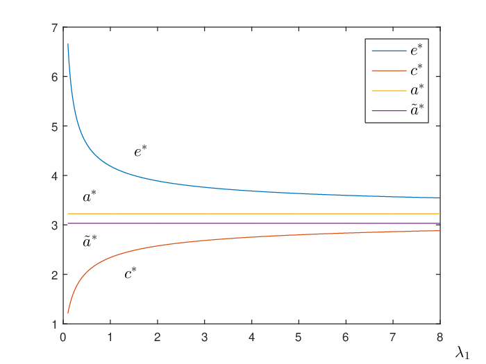
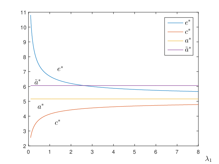
First, we conduct a sensitivity analysis of the thresholds with respect to the early termination rate λ1\lambda_{1}. As is seen in Figure 3, the pre/post-competition abandonment levels do not change with λ1\lambda_{1} since the firm has already entered the market. For the entry and cancellation thresholds, we see that e∗e^{*} decreases but c∗c^{*} increases as λ1\lambda_{1} increases. In other words, a high early termination risk induces the firm to enter the market early, even if that means capturing a lower profit stream upon entry. Moreover, the firm may also cancel the project earlier because the expected profitability is reduced by the higher termination risk. In Figure 3, we also observe that the threshold e∗e^{*} is higher than a∗a^{*} while c∗c^{*} is lower than a∗a^{*}.

Figures 3(a) and 3(b) depict the two cases a~∗≤a∗\widetilde{a}^{*}\leq a^{*} and a~∗>a∗\widetilde{a}^{*}>a^{*} respectively. The impact of early termination risk is different in these two scenarios. If the competitor’s entry causes a significant shrinkage in the firm’s profit as in case (II), then the post-competition abandonment level a~∗\widetilde{a}^{*} will be higher than the pre-competition one a∗a^{*}. Also, the firm’s entry level e∗e^{*} is decreasing in λ1\lambda_{1}. In Figure 3(b), we see that e∗e^{*} will eventually fall below a~∗\widetilde{a}^{*} but stay above a∗a^{*}. In this case, whenever the competitor enters, the firm switches its abandonment level to the higher level a~∗\widetilde{a}^{*}. This forces the firm to abandon immediately involuntarily if the current value of XX is below a~∗\widetilde{a}^{*}.

Refer to caption
(a) Case (I): a~∗≤a∗\widetilde{a}^{*}\leq a^{*}. α=0.6\alpha=0.6, β=7\beta=7.
Refer to caption
(b) Case (II): a~∗>a∗\widetilde{a}^{*}>a^{*}. α=0.3\alpha=0.3, β=7\beta=7.
Figure 3: Sensitivity of the firm’s strategies with respect to early termination rate λ1\lambda_{1}.

5.2 Competition Risk

The risk of competition will influence the firm’s pre-competition exit strategy, described by a∗a^{*}, in a non-trivial way. We discuss the four scenarios of different sensitivities in Figure 4. In the following discussion, we keep in mind that a~∗\widetilde{a}^{*} doesn’t depend on λ2\lambda_{2} and α0\alpha_{0} is decreasing in λ2\lambda_{2} by Corollary 3.5.

Figure 4(a) illustrates the first scenario with K<βK<\beta. This corresponds to case (II) in Proposition 3.4, where we have shown that a∗<a~∗a^{*}<\widetilde{a}^{*} for all λ2>0\lambda_{2}>0. In addition, a∗a^{*} is increasing in λ2\lambda_{2}, which means that the firm will choose to exit early under the threat of competitor’s entry.

For the remaining three scenarios in Figures 4(b)-4(d), we have K≥βK\geq\beta. By Corollary 3.5, we have 1>α0​(0)>α0​(λ2)>α0∞>01>\alpha_{0}(0)>\alpha_{0}(\lambda_{2})>\alpha^{\infty}_{0}>0 for all λ2>0\lambda_{2}>0. In Figure 4(b), a∗a^{*} is again increasing in λ2\lambda_{2}. In this figure, we have α≤α0∞\alpha\leq\alpha^{\infty}_{0}, which belongs to case (II) in Proposition 3.4, and thus a∗<a~∗a^{*}<\widetilde{a}^{*}.

Figure 4(c) shows that a∗a^{*} is first increasing then decreasing in λ2\lambda_{2}. This is because the constant α0\alpha_{0} is first larger than α\alpha but then smaller than α\alpha as λ2\lambda_{2} increases. Therefore, as λ2\lambda_{2} increases, it changes from case (II) to case (I) in Proposition 3.4. That explains why a∗a^{*} is smaller than a~∗\widetilde{a}^{*} at first, and the relation reverses for large λ2\lambda_{2}.

Lastly, in Figure 4(d) we have α≥α0​(0)\alpha\geq\alpha_{0}(0), which corresponds to case (I) in Proposition 3.4. We have shown that a∗≥a~∗a^{*}\geq\widetilde{a}^{*} for all λ2\lambda_{2}. In contrast to the other scenarios, the pre-competition threshold a∗a^{*} is decreasing and approaches a~∗\widetilde{a}^{*} as λ2\lambda_{2} increases. In this scenario, the impact of the competitor’s entry on the firm’s profit is much less than in other scenarios, as indicated by the higher value of α\alpha.

In summary, scenarios (a), (b), and the first part of scenario (c) belong to case (II), in which the competitor’s potential entry will lead to a significant profit reduction. Therefore, the firm exits early by selecting a higher pre-competition abandonment threshold a∗a^{*} as the competitor’s arrival rate increases. The opposite happens to scenario (d) and the second part (large λ2\lambda_{2}) of scenario (c). As λ2\lambda_{2} increases, which means high risk of facing competition in the future, the firm tries to stay longer before the competitor’s entry to make more profits in case of the potential significant loss afterwards. This results in a decreasing pre-competition abandonment threshold a∗a^{*}.

Despite different behaviors of a∗a^{*}, there is a common phenomenon that a∗a^{*} approaches a~∗\widetilde{a}^{*} as λ2\lambda_{2} increases. The intuitive explanation is as follows. When the competition risk is very high, the firm will adjust its abandonment level a∗a^{*} in order not to be affected too much when the competitor eventually enters. That means that the firm’s abandonment level a∗a^{*} before the competitor’s entry will be close to the post-competition abandonment level a~∗\widetilde{a}^{*}.

Refer to caption
(a) α=0.20\alpha=0.20, β=14\beta=14.
Refer to caption
(b) α=0.20\alpha=0.20, β=7\beta=7.
Refer to caption
(c) α=0.45\alpha=0.45, β=7\beta=7.
Refer to caption
(d) α=0.80\alpha=0.80, β=7\beta=7.
Figure 4: Sensitivity of the abandonment thresholds, a∗a^{*} (pre-competition) and a~∗\widetilde{a}^{*} (post-competition), with respect to the competitor’s arrival rate λ2\lambda_{2}.

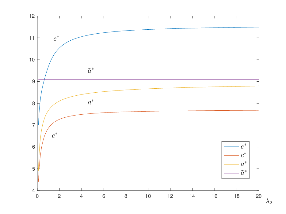
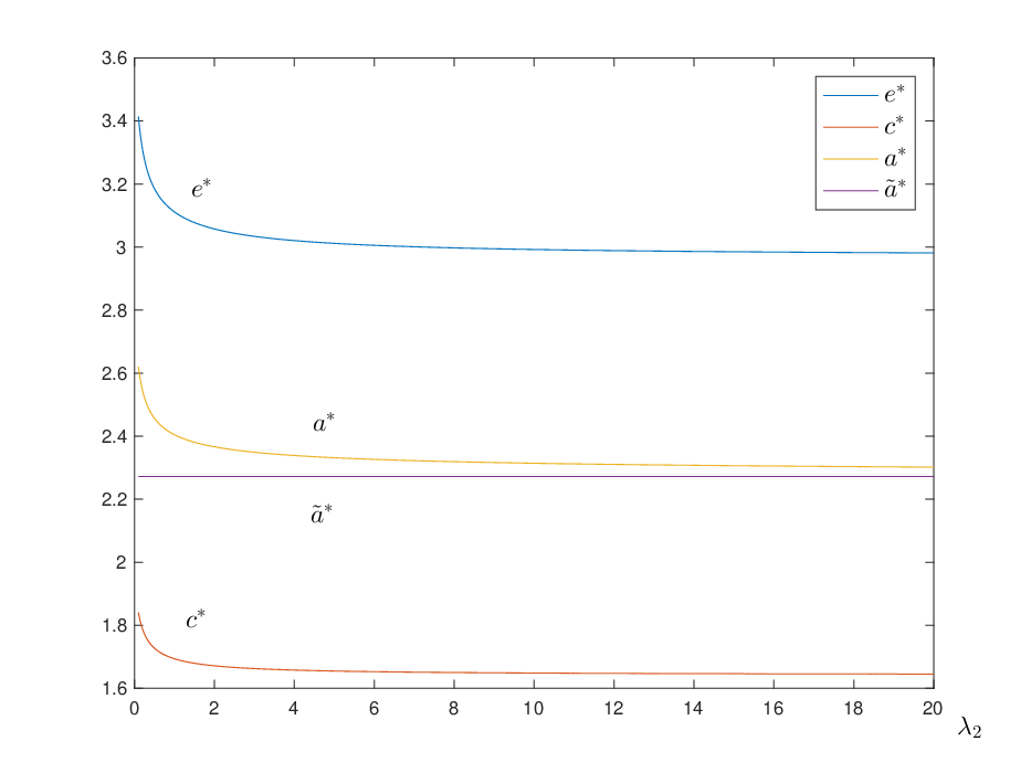
In addition to a∗a^{*}, the entry and cancellation thresholds e∗e^{*} and c∗c^{*} are also affected by the competitor’s arrival rate λ2\lambda_{2} after the firm’s market entry. In two scenarios, Figure 5(a) and Figure 5(b) respectively take the same parameters as Figure 4(b) and Figure 4(d), so they represent respectively case (II) and (I) in Proposition 3.4. Figure 5(a) shows that both e∗e^{*} and c∗c^{*} are increasing in λ2\lambda_{2} under case (II). In particular, the entry threshold e∗e^{*} is seen to be lower than the abandonment threshold a~∗\widetilde{a}^{*} when λ2\lambda_{2} is small, but then surpasses it for large λ2\lambda_{2}. In this case, the competitor’s arrival will lead to a significant post-entry profit reduction. Therefore, as is intuitive, the firm requires a higher entry level to ensure a higher post-entry profit so as to make the entry worthwhile. Nevertheless, under case (I), Figure 5(b) shows that both e∗e^{*} and c∗c^{*} are decreasing in λ2\lambda_{2}. In other words, when the post-entry competition arrival is not expected to have a significant impact on profit, the firm will opt to enter the market earlier at a lower entry threshold.
Refer to caption
(a) α=0.20\alpha=0.20, β=7\beta=7.
Refer to caption
(b) α=0.80\alpha=0.80, β=7\beta=7.
Figure 5: Sensitivity of the entry and cancellation thresholds, e∗e^{*} and c∗{c}^{*}, with respect to the competitor’s arrival rate λ2\lambda_{2}.

6 Concluding Remarks

We have developed a model to evaluate the timing options to enter or exit a given market for a startup firm. Our model accounts for the risks of early termination prior to market entry, as well as the risk of new competition that may reduce the firm’s future profit stream. Our analytic solutions allow for instant computation of the firm’s optimal expected NPV and the associated optimal timing strategies. We have provided explanation on the non-trivial combined effect of early termination and competition risks on the firm’s entry and pre-competition abandonment decisions.

There are a number of directions for future research. For tractability, we have chosen to work with a lognormal model. Alternatively, we will consider in future work other dynamics for the underlying price process, such as jump diffusions or mean-reverting processes, such as the Cox-Ingersoll-Ross, and exponential Ornstein-Uhlenbeck processes (Leung et al. (2014), Leung et al. (2015)). For a startup, it is also useful to choose between equity and debt financing and examine the implications to the firm’s investment and bankruptcy decisions (see, e.g. Tian (2011)). Another natural extension of our model is to incorporate sequential random arrivals and departures of competitors.

Appendix A Appendix

In this appendix, we provide the proofs of all the propositions and corollaries presented above.

A.1 Proof of Equations (2.3) and (2.4)

Recall that (ℱt)t≥0({\cal{F}}_{t})_{t\geq 0} is the filtration generated by XX. We re-state equation (2.3), and apply the tower property to get

V⁡(x)\displaystyle V(x) =supτa∈𝒯𝔼x[∫0τa∧ζ2𝐞−ρ​tf(Xt)dt+11{τa>ζ2}𝐞−ρ​ζ2V~(Xζ2)]\displaystyle=\sup_{\begin{subarray}{c}\tau_{a}\in\cal{T}\end{subarray}}\mathbb{E}_{x}\left[\int_{0}^{\tau_{a}\wedge\zeta_{2}}\mathbf{e}^{-\rho t}f\left(X_{t}\right)\,dt+1\hskip-5.97508pt{1}_{\{\tau_{a}>\zeta_{2}\}}\mathbf{e}^{-\rho\zeta_{2}}\widetilde{V}(X_{\zeta_{2}})\,\right]
=supτa∈𝒯𝔼x[𝔼[∫0τa∧ζ2𝐞−ρ​tf(Xt)dt+11{τa>ζ2}𝐞−ρ​ζ2V~(Xζ2)|ℱτa]].\displaystyle=\sup_{\begin{subarray}{c}\tau_{a}\in\cal{T}\end{subarray}}\mathbb{E}_{x}\left[\mathbb{E}\left[\int_{0}^{\tau_{a}\wedge\zeta_{2}}\mathbf{e}^{-\rho t}f\left(X_{t}\right)\,dt+1\hskip-5.97508pt{1}_{\{\tau_{a}>\zeta_{2}\}}\mathbf{e}^{-\rho\zeta_{2}}\widetilde{V}(X_{\zeta_{2}})~\Big|{\cal{F}}_{\tau_{a}}\right]\right]. (A.1)

The arrival time ζ2\zeta_{2} is exponentially distributed and independent of XX, so the first term inside the expectation (A.1) can be written as

𝔼⁡[∫0τa∧ζ2𝐞−ρ​t​f​(Xt)​𝑑t|ℱτa]\displaystyle\mathbb{E}\left[\int_{0}^{\tau_{a}\wedge\zeta_{2}}\mathbf{e}^{-\rho t}f\left(X_{t}\right)\,dt~\Big|{\cal{F}}_{\tau_{a}}\right] =𝔼[∫0τa11{ζ2≥t}𝐞−ρ​tf(Xt)dt|ℱτa]\displaystyle=\mathbb{E}\left[\int_{0}^{\tau_{a}}1\hskip-5.97508pt{1}_{\{\zeta_{2}\geq t\}}\mathbf{e}^{-\rho t}f\left(X_{t}\right)\,dt~\Big|{\cal{F}}_{\tau_{a}}\right]
=𝔼⁡[∫0τa(∫t+∞λ2​𝐞−λ2​y​𝑑y)​𝐞−ρ​t​f​(Xt)​𝑑t|ℱτa]\displaystyle=\mathbb{E}\left[\int_{0}^{\tau_{a}}\left(\int_{t}^{+\infty}\lambda_{2}\mathbf{e}^{-\lambda_{2}y}\,dy\right)\mathbf{e}^{-\rho t}f\left(X_{t}\right)\,dt~\Big|{\cal{F}}_{\tau_{a}}\right]
=𝔼⁡[∫0τa𝐞−(λ2+ρ)​t​f​(Xt)​𝑑t|ℱτa].\displaystyle=\mathbb{E}\left[\int_{0}^{\tau_{a}}\mathbf{e}^{-(\lambda_{2}+\rho)t}f\left(X_{t}\right)\,dt~\Big|{\cal{F}}_{\tau_{a}}\right]. (A.2)

By the same procedure, we express the second term in (A.1) as

𝔼[11{τa>ζ2}𝐞−ρ​ζ2V~(Xζ2)|ℱτa]=𝔼[∫0τa𝐞−(λ2+ρ)​tλ2V~(Xt)dt|ℱτa].\mathbb{E}\left[1\hskip-5.97508pt{1}_{\{\tau_{a}>\zeta_{2}\}}\mathbf{e}^{-\rho\zeta_{2}}\widetilde{V}(X_{\zeta_{2}})~\Big|{\cal{F}}_{\tau_{a}}\right]=\mathbb{E}\left[\int_{0}^{\tau_{a}}\mathbf{e}^{-(\lambda_{2}+\rho)t}\lambda_{2}\widetilde{V}(X_{t})\,dt~\Big|{\cal{F}}_{\tau_{a}}\right]. (A.3)

Combining (A.2) and (A.3), we obtain equation (2.3). Equation (2.4) is derived in the same fashion.

A.2 Proof of Proposition 3.1

Proof.

We consider a candidate stopping time τ~a=inf{t≥0:Xt≤a~∗}\widetilde{\tau}_{a}=\inf\{t\geq 0:X_{t}\leq\widetilde{a}^{*}\}, where a~∗>0\widetilde{a}^{*}>0. In the stopping region {x<a~∗}\{x<\widetilde{a}^{*}\}, V~​(x)=0\widetilde{V}(x)=0 from the definition of τ~a\widetilde{\tau}_{a} and (2.2). In the continuation region {x≥a~∗}\{x\geq\widetilde{a}^{*}\}, V~​(x)\widetilde{V}(x) satisfies the following ODE:

−ρ​V~​(x)+μ​x​V~′​(x)+σ2​x22​V~′′​(x)+g⁡(x)=0,-\rho\widetilde{V}(x)+\mu x\widetilde{V}^{\prime}(x)+\frac{\sigma^{2}x^{2}}{2}\widetilde{V}^{\prime\prime}(x)+g(x)=0, (A.4)

with boundary conditions:

V~​(a~∗)=0,V~′​(a~∗)=0,limx→∞V~′​(x)<∞.\displaystyle\widetilde{V}(\widetilde{a}^{*})=0,\,\,\,\,\,\,\widetilde{V}^{\prime}(\widetilde{a}^{*})=0,\,\,\,\,\,\,\lim_{x\to\infty}\widetilde{V}^{\prime}(x)<\infty. (A.5)

The ODE and the last condition in (A.5) indicate that the solution is given by B1​xk1+g0​(x)B_{1}x^{k_{1}}+g_{0}(x), where with constants B1B_{1} and k1k_{1}, such that k1k_{1} is the negative root of the associated quadratic equation, and g0​(x)g_{0}(x) is a particular solution of (A.4):

g0​(x)=α​xρ−μ−βρ.g_{0}(x)=\frac{\alpha x}{\rho-\mu}-\frac{\beta}{\rho}. (A.6)

To determine a~∗\widetilde{a}^{*} and B1B_{1}, we utilize boundary conditions (A.5) to get the system of equations:

B1​(a~∗)k1+α​a~∗ρ−μ+βρ\displaystyle B_{1}(\widetilde{a}^{*})^{k_{1}}+\frac{\alpha\widetilde{a}^{*}}{\rho-\mu}+\frac{\beta}{\rho} =0,\displaystyle=0, (A.7)
B1​k1​(a~∗)k1−1+αρ−μ\displaystyle B_{1}k_{1}(\widetilde{a}^{*})^{k_{1}-1}+\frac{\alpha}{\rho-\mu} =0.\displaystyle=0. (A.8)

The above equations yield (3.3) and (3.4) in Proposition 3.1.∎

A.3 Proof of Corollary 3.2

Proof.

First, we define the ratio:

k1k1−1\displaystyle\frac{k_{1}}{k_{1}-1} =(1+σ2​((σ22−μ)2+2​σ2​ρ−σ22+μ)−1)−1.\displaystyle=\left(1+\sigma^{2}\left(\sqrt{(\frac{\sigma^{2}}{2}-\mu)^{2}+2\sigma^{2}\rho}-\frac{\sigma^{2}}{2}+\mu\right)^{-1}\right)^{-1}. (A.9)

From (A.9) and the expression of a~∗\widetilde{a}^{*} in (3.4), we know that k1k1−1\frac{k_{1}}{k_{1}-1} increases in ρ\rho and thus a~∗\widetilde{a}^{*} increases in ρ\rho.

Next, we differentiate a~∗\widetilde{a}^{*} with respect to μ\mu. Let δ:=(σ22−μ)2+2​σ2​ρ>|σ22−μ|≥0\delta:=\sqrt{(\frac{\sigma^{2}}{2}-\mu)^{2}+2\sigma^{2}\rho}>|\frac{\sigma^{2}}{2}-\mu|\geq 0, then

∂a~∗∂μ=−2​βα​(2​ρ+σ22−μ+δ)2​(σ22+δ+(ρ​δ+(ρ−μ)​(μ−σ22))​δ−1).\frac{\partial{\widetilde{a}^{*}}}{\partial{\mu}}=\frac{-2\beta}{\alpha(2\rho+\frac{\sigma^{2}}{2}-\mu+\delta)^{2}}\left(\frac{\sigma^{2}}{2}+\delta+(\rho\delta+(\rho-\mu)(\mu-\frac{\sigma^{2}}{2}))\delta^{-1}\right). (A.10)

Since ρ​δ>|(ρ−μ)​(μ−σ22)|\rho\delta>|(\rho-\mu)(\mu-\frac{\sigma^{2}}{2})|, we have ∂a~∗∂μ<0\frac{\partial{\widetilde{a}^{*}}}{\partial{\mu}}<0 and thus a~∗\widetilde{a}^{*} decreases with respect to μ\mu.

In addition,

∂k1∂σ=∂k1∂(σ2)​∂(σ2)∂σ=σ22−μ+δ+2​ρ2​ρ​k12​σ>0.\frac{\partial k_{1}}{\partial\sigma}=\frac{\partial k_{1}}{\partial{(\sigma^{2})}}\frac{\partial{(\sigma^{2})}}{\partial\sigma}=\frac{\frac{\sigma^{2}}{2}-\mu+\delta+2\rho}{2\rho}k_{1}^{2}\sigma>0. (A.11)

Therefore k1<0k_{1}<0 and ∂k1∂σ>0\frac{\partial k_{1}}{\partial\sigma}>0 indicate that k1k1−1\frac{k_{1}}{k_{1}-1} decreases in σ\sigma and thus a~∗\widetilde{a}^{*} decreases in σ\sigma.

Finally, that a~∗\widetilde{a}^{*} decreases in α\alpha and increases in β\beta can be directly inferred from (3.4). ∎

A.4 Proof of Corollary 3.3

Proof.

We take the first and second derivatives of V~​(x)\widetilde{V}(x), namely,

V~′​(x)=αρ−μ​(1−(a~∗x)1−k1)and V~′′​(x)=α⁡(1−k1)ρ−μ​(a~∗)1−k1​xk1−2,∀x>a~∗.\displaystyle\widetilde{V}^{\prime}(x)=\frac{\alpha}{\rho-\mu}\left(1-\left(\frac{\widetilde{a}^{*}}{x}\right)^{1-k_{1}}\right)\quad\text{and }\quad\widetilde{V}^{\prime\prime}(x)=\frac{\alpha(1-k_{1})}{\rho-\mu}(\widetilde{a}^{*})^{1-k_{1}}x^{k_{1}-2}\,,\quad\forall x>\widetilde{a}^{*}. (A.12)

In turn, k1<0k_{1}<0 implies V~′​(x)>0\widetilde{V}^{\prime}(x)>0 and V~′′​(x)>0\widetilde{V}^{\prime\prime}(x)>0 for all x>a~∗x>\widetilde{a}^{*}. In addition, when xx is sufficient large, the first part of V~​(x)\widetilde{V}(x) is negligible and its sensitivity with respect to the parameters can be deduced from (3.3). ∎

A.5 Proof of Proposition 3.4

To prove Proposition 3.4, we first establish the following lemmas.

Lemma A.1.

Let H:ℝ+→ℝH:\mathbb{R}_{+}\to\mathbb{R} such that

H⁡(x)=α⁡(k1−p1)k1​(ρ−μ)​(a~∗)1−k1​xk1+ρ+α​λ2−μρ+λ2−μ​p1−1ρ−μ​x−p1​(β​λ2+ρ​K)ρ⁡(ρ+λ2),H(x)=\frac{\alpha(k_{1}-p_{1})}{k_{1}(\rho-\mu)}(\widetilde{a}^{*})^{1-k_{1}}x^{k_{1}}+\frac{\rho+\alpha\lambda_{2}-\mu}{\rho+\lambda_{2}-\mu}\frac{p_{1}-1}{\rho-\mu}x-\frac{p_{1}(\beta\lambda_{2}+\rho K)}{\rho(\rho+\lambda_{2})}, (A.13)

then there exists unique a∗∈[a~∗,+∞)a^{*}\in[\widetilde{a}^{*},+\infty), such that H⁡(a∗)=0H(a^{*})=0, if and only if K≥βK\geq\beta and α0≤α≤1\alpha_{0}\leq\alpha\leq 1. If α=α0\alpha=\alpha_{0}, then a∗=a~∗a^{*}=\widetilde{a}^{*}.

Proof.

We take the first and second derivatives of H⁡(x)H(x),

H′​(x)\displaystyle H^{\prime}(x) =α⁡(k1−p1)ρ−μ​(a~∗)1−k1​xk1−1+ρ+α​λ2−μρ+λ2−μ​p1−1ρ−μ,\displaystyle=\frac{\alpha(k_{1}-p_{1})}{\rho-\mu}(\widetilde{a}^{*})^{1-k_{1}}x^{k_{1}-1}+\frac{\rho+\alpha\lambda_{2}-\mu}{\rho+\lambda_{2}-\mu}\frac{p_{1}-1}{\rho-\mu}, (A.14)
H′′​(x)\displaystyle H^{\prime\prime}(x) =α⁡(k1−p1)​(k1−1)ρ−μ​(a~∗)1−k1​xk1−2.\displaystyle=\frac{\alpha(k_{1}-p_{1})(k_{1}-1)}{\rho-\mu}(\widetilde{a}^{*})^{1-k_{1}}x^{k_{1}-2}. (A.15)

Notice α>0\alpha>0 and p1<k1<0p_{1}<k_{1}<0, then H′′​(x)<0H^{\prime\prime}(x)<0 for all x>0x>0. This means H′​(x)H^{\prime}(x) is a decreasing function with respect to xx. By inspection, we have

H′​(x)​{>0if 0<x<a0∗,=0if x=a0∗,<0if x>a0∗, with​a0∗=a~∗​(1−p1α⁡(k1−p1)​ρ+α​λ2−μρ+λ2−μ)1k1−1.H^{\prime}(x)\begin{cases}>0&\mbox{if $0<x<{a}^{*}_{0}$,}\\ =0&\mbox{if $x={a}^{*}_{0}$,}\\ <0&\mbox{if $x>{a}^{*}_{0}$,}\\ \end{cases}\quad\text{ with}~~{a}^{*}_{0}=\widetilde{a}^{*}\left(\frac{1-p_{1}}{\alpha(k_{1}-p_{1})}\frac{\rho+\alpha\lambda_{2}-\mu}{\rho+\lambda_{2}-\mu}\right)^{\frac{1}{k_{1}-1}}\,. (A.16)

The derivative means that H⁡(x)H(x) is unimodal and maximized at a0∗{a}^{*}_{0}. Moreover, we have limx→0H⁡(x)=limx→+∞H⁡(x)=−∞\lim_{x\to 0}H(x)=\lim_{x\to+\infty}H(x)=-\infty. Note that (1−p1α⁡(k1−p1)​ρ+α​λ2−μρ+λ2−μ)\left(\frac{1-p_{1}}{\alpha(k_{1}-p_{1})}\frac{\rho+\alpha\lambda_{2}-\mu}{\rho+\lambda_{2}-\mu}\right) is a decreasing function of α⁡(0<α≤1)\alpha~(0<\alpha\leq 1). When α=1\alpha=1, (1−p1α⁡(k1−p1)​ρ+α​λ2−μρ+λ2−μ)>1\left(\frac{1-p_{1}}{\alpha(k_{1}-p_{1})}\frac{\rho+\alpha\lambda_{2}-\mu}{\rho+\lambda_{2}-\mu}\right)>1. Therefore, we see that a0∗<a~∗{a}^{*}_{0}<\widetilde{a}^{*} for all 0<α≤10<\alpha\leq 1.

There exists a unique a∗a^{*} such that H⁡(a∗)=0H(a^{*})=0 and a∗≥a~∗a^{*}\geq\widetilde{a}^{*} if and only if H⁡(a~∗)≥0H(\widetilde{a}^{*})\geq 0. To see this, if there is an a∗≥a~∗a^{*}\geq\widetilde{a}^{*} such that H⁡(a∗)=0H(a^{*})=0, then H⁡(a~∗)≥0H(\widetilde{a}^{*})\geq 0, because H⁡(x)H(x) is a decreasing function when x>a0∗x>{a}^{*}_{0} and a∗≥a~∗>a0∗a^{*}\geq\widetilde{a}^{*}>{a}^{*}_{0}. On the other hand, if H⁡(a~∗)≥0H(\widetilde{a}^{*})\geq 0, the existence and uniqueness of a∗a^{*} comes from the fact that H⁡(x)H(x) is continuous and decreasing for x>a~∗>a0∗x>\widetilde{a}^{*}>{a}^{*}_{0}, along with limx→+∞H⁡(x)=−∞\lim_{x\to+\infty}H(x)=-\infty.

Now H⁡(a~∗)H(\widetilde{a}^{*}) is given by

H⁡(a~∗)=β⁡(p1−k1)ρ⁡(1−k1)+k1​β​(ρ+α​λ2−μ)​(1−p1)ρ​α​(ρ+λ2−μ)​(1−k1)−p1​(β​λ2+ρ​K)ρ⁡(ρ+λ2).H(\widetilde{a}^{*})=\frac{\beta(p_{1}-k_{1})}{\rho(1-k_{1})}+\frac{k_{1}\beta(\rho+\alpha\lambda_{2}-\mu)(1-p_{1})}{\rho\alpha(\rho+\lambda_{2}-\mu)(1-k_{1})}-\frac{p_{1}(\beta\lambda_{2}+\rho K)}{\rho(\rho+\lambda_{2})}. (A.17)

It’s easy to see that H⁡(a~∗)H(\widetilde{a}^{*}) is increasing in α⁡(0≤α≤1)\alpha~(0\leq\alpha\leq 1), holding other parameters fixed. When α=1\alpha=1, H⁡(a~∗)|α=1=p1​(β−K)(λ2+ρ)H(\widetilde{a}^{*})|_{\alpha=1}=\frac{p_{1}(\beta-K)}{(\lambda_{2}+\rho)}, which means H⁡(a~∗)≤p1​(β−K)(λ2+ρ)H(\widetilde{a}^{*})\leq\frac{p_{1}(\beta-K)}{(\lambda_{2}+\rho)} for all 0≤α≤10\leq\alpha\leq 1.
(1)(1) If K<βK<\beta, then H⁡(a~∗)<0H(\widetilde{a}^{*})<0, and there is not an a∗≥a~∗a^{*}\geq\widetilde{a}^{*} such that H⁡(a∗)=0H(a^{*})=0.
(2)(2) If K≥βK\geq\beta, then

H⁡(a~∗)​{>0if α>α0,=0if α=α0,<0if α<α0, with ​α0=(1−ρ​p1​(k1−1)​(ρ+λ2−μ)k1​(p1−1)​(ρ−μ)​(ρ+λ2)​(1−Kβ))−1.H(\widetilde{a}^{*})\begin{cases}>0&\mbox{if $\alpha>\alpha_{0}$,}\\ =0&\mbox{if $\alpha=\alpha_{0}$,}\\ <0&\mbox{if $\alpha<\alpha_{0}$,}\\ \end{cases}\quad\text{ with }~~\alpha_{0}=\left(1-\frac{\rho p_{1}(k_{1}-1)(\rho+\lambda_{2}-\mu)}{k_{1}(p_{1}-1)(\rho-\mu)(\rho+\lambda_{2})}(1-\frac{K}{\beta})\right)^{-1}\,. (A.18)

From cases (1)(1) and (2)(2) above, we conclude that K≥βK\geq\beta and α0≤α≤1\alpha_{0}\leq\alpha\leq 1 iff H⁡(a~∗)≥0H(\widetilde{a}^{*})\geq 0 iff there exists a unique a∗a^{*} such that H⁡(a∗)=0H(a^{*})=0 and a∗≥a~∗a^{*}\geq\widetilde{a}^{*}. Moreover, a∗=a~∗a^{*}=\widetilde{a}^{*} iff K≥βK\geq\beta and α=α0\alpha=\alpha_{0}, due to the uniqueness of a∗a^{*}. ∎

Lemma A.2.

Let M:ℝ+→ℝM:\mathbb{R}_{+}\to\mathbb{R} such that

M⁡(x)=(p1−k1)​ρ​(ρ+λ2−μ)+k1​μ​λ2​(1−p1)(1−k1)​ρ​(ρ+λ2)​(ρ+λ2−μ)​β​(a~∗)−p2​xp2+p1−1ρ+λ2−μ​x−p1​Kρ+λ2,M(x)=\frac{(p_{1}-k_{1})\rho(\rho+\lambda_{2}-\mu)+k_{1}\mu\lambda_{2}(1-p_{1})}{(1-k_{1})\rho(\rho+\lambda_{2})(\rho+\lambda_{2}-\mu)}\beta(\widetilde{a}^{*})^{-p_{2}}x^{p_{2}}+\frac{p_{1}-1}{\rho+\lambda_{2}-\mu}x-\frac{p_{1}K}{\rho+\lambda_{2}}, (A.19)

then there exists unique a∗∈(0,a~∗)a^{*}\in(0,\widetilde{a}^{*}), such that M⁡(a∗)=0M(a^{*})=0, if and only if K<βK<\beta, or K≥βK\geq\beta and 0≤α<α00\leq\alpha<\alpha_{0}.

Proof.

We take the first derivative of M⁡(x)M(x),

M′​(x)=(p1−k1)​ρ​(ρ+λ2−μ)+k1​μ​λ2​(1−p1)(1−k1)​ρ​(ρ+λ2)​(ρ+λ2−μ)​β​(a~∗)−p2​p2​xp2−1+p1−1ρ+λ2−μ.M^{\prime}(x)=\frac{(p_{1}-k_{1})\rho(\rho+\lambda_{2}-\mu)+k_{1}\mu\lambda_{2}(1-p_{1})}{(1-k_{1})\rho(\rho+\lambda_{2})(\rho+\lambda_{2}-\mu)}\beta(\widetilde{a}^{*})^{-p_{2}}p_{2}x^{p_{2}-1}+\frac{p_{1}-1}{\rho+\lambda_{2}-\mu}. (A.20)

Conditions μ>0\mu>0, p1<k1<0p_{1}<k_{1}<0 and p2>1p_{2}>1 indicate M′​(x)<0M^{\prime}(x)<0 for all x>0x>0 and thus M⁡(x)M(x) is a decreasing function in xx. M⁡(0)=−p1​Kρ+λ2>0M(0)=-\frac{p_{1}K}{\rho+\lambda_{2}}>0 and limx→∞M⁡(x)=−∞\lim_{x\to\infty}M(x)=-\infty imply that there exists unique a∗a^{*} such that M⁡(a∗)=0M(a^{*})=0.

Now we need to check whether a~∗>a∗\widetilde{a}^{*}>a^{*} or not. Note a~∗>a∗\widetilde{a}^{*}>a^{*} if and only if M⁡(a~∗)<0M(\widetilde{a}^{*})<0.

M⁡(a~∗)=\displaystyle M(\widetilde{a}^{*})= (p1−k1)​ρ​(ρ+λ2−μ)+k1​μ​λ2​(1−p1)(1−k1)​ρ​(ρ+λ2)​(ρ+λ2−μ)​β+p1−1ρ+λ2−μ​a~∗−p1​Kρ+λ2\displaystyle\frac{(p_{1}-k_{1})\rho(\rho+\lambda_{2}-\mu)+k_{1}\mu\lambda_{2}(1-p_{1})}{(1-k_{1})\rho(\rho+\lambda_{2})(\rho+\lambda_{2}-\mu)}\beta+\frac{p_{1}-1}{\rho+\lambda_{2}-\mu}\widetilde{a}^{*}-\frac{p_{1}K}{\rho+\lambda_{2}}
=\displaystyle= (p1−k1)​ρ​(ρ+λ2−μ)+k1​μ​λ2​(1−p1)(1−k1)​ρ​(ρ+λ2)​(ρ+λ2−μ)​β+p1−1ρ+λ2−μ​ρ−μρ​k1k1−1​βα−p1​Kρ+λ2.\displaystyle\frac{(p_{1}-k_{1})\rho(\rho+\lambda_{2}-\mu)+k_{1}\mu\lambda_{2}(1-p_{1})}{(1-k_{1})\rho(\rho+\lambda_{2})(\rho+\lambda_{2}-\mu)}\beta+\frac{p_{1}-1}{\rho+\lambda_{2}-\mu}\frac{\rho-\mu}{\rho}\frac{k_{1}}{k_{1}-1}\frac{\beta}{\alpha}-\frac{p_{1}K}{\rho+\lambda_{2}}. (A.21)

It’s easy to check that M⁡(a~∗)=H⁡(a~∗)M(\widetilde{a}^{*})=H(\widetilde{a}^{*}) (in the proof of Lemma A.1). Follow the last part of the proof in Lemma A.1, we immediately obtain the result of Lemma A.2. ∎

Now let’s focus on the proof of Proposition 3.4.

Proof.

We consider a candidate stopping time τa=inf{t≥0:Xt≤a∗}\tau_{a}=\inf\{t\geq 0:X_{t}\leq a^{*}\}, where a∗>0a^{*}>0. We split the problem into two cases: a∗≥a~∗a^{*}\geq\widetilde{a}^{*} and a∗<a~∗a^{*}<\widetilde{a}^{*}.

(I) We first assume a∗≥a~∗a^{*}\geq\widetilde{a}^{*}. In the stopping region {x<a∗}\{x<a^{*}\}, V⁡(x)=0V(x)=0 from the definition τa\tau_{a} and (2.3). In the continuation region {x≥a∗}\{x\geq a^{*}\}, V⁡(x)V(x) satisfies the following ODE:

−(ρ+λ2)​V​(x)+μ​x​V′​(x)+σ2​x22​V′′​(x)+f⁡(x)+λ2​V~​(x)=0,-(\rho+\lambda_{2})V(x)+\mu xV^{\prime}(x)+\frac{\sigma^{2}x^{2}}{2}V^{\prime\prime}(x)+f(x)+\lambda_{2}\widetilde{V}(x)=0, (A.22)

with boundary conditions:

V⁡(a∗)=0,V′​(a∗)=0,limx→∞V′​(x)<+∞.\displaystyle V(a^{*})=0,\,\,\,\,\,\,V^{\prime}(a^{*})=0,\,\,\,\,\,\,\lim_{x\to\infty}V^{\prime}(x)<+\infty. (A.23)

The ODE and last condition in (A.23) indicate that the general solution is given by C1​xp1+v1​(x)C_{1}x^{p_{1}}+v_{1}(x), where C1C_{1} is a constant, p1p_{1} is the negative root of the associated quadratic equation, and v1​(x)v_{1}(x) is a particular solution of (A.22):

v1​(x)=−αk1​(ρ−μ)​(a~∗)1−k1​xk1+ρ+α​λ2−μρ+λ2−μ​1ρ−μ​x−β​λ2+ρ​Kρ⁡(ρ+λ2).v_{1}(x)=-\frac{\alpha}{k_{1}(\rho-\mu)}(\widetilde{a}^{*})^{1-k_{1}}x^{k_{1}}+\frac{\rho+\alpha\lambda_{2}-\mu}{\rho+\lambda_{2}-\mu}\frac{1}{\rho-\mu}x-\frac{\beta\lambda_{2}+\rho K}{\rho(\rho+\lambda_{2})}. (A.24)

To determine a∗a^{*} and C1C_{1}, we utilize boundary conditions (A.23) to get the following system of equations:

C1​(a∗)p1+v1​(a∗)\displaystyle C_{1}(a^{*})^{p_{1}}+v_{1}(a^{*}) =0,\displaystyle=0, (A.25)
C1​p1​(a∗)p1−1+v1′​(a∗)\displaystyle C_{1}p_{1}(a^{*})^{p_{1}-1}+v_{1}^{\prime}(a^{*}) =0.\displaystyle=0. (A.26)

The above equations yield (3.7). From Lemma A.1, if K≥βK\geq\beta and α0≤α≤1\alpha_{0}\leq\alpha\leq 1, then there exists unique a∗≥a~∗a^{*}\geq\widetilde{a}^{*}, satisfying (3.7). We solve a∗a^{*} numerically and plug it in (A.25) and (A.26), then we can get (3.12) and thus (3.8).

(II) Next we assume a∗<a~∗a^{*}<\widetilde{a}^{*}. Also from the definition τa\tau_{a} and (2.3), V⁡(x)=0V(x)=0 in the stopping region {x<a∗}\{x<a^{*}\}. In the continuation region {x≥a∗}\{x\geq a^{*}\}, V⁡(x)V(x) satisfies the following ODE:

−(ρ+λ2)​V​(x)+μ​x​V′​(x)+σ2​x22​V′′​(x)+f⁡(x)+λ2​V~​(x)=0,-(\rho+\lambda_{2})V(x)+\mu xV^{\prime}(x)+\frac{\sigma^{2}x^{2}}{2}V^{\prime\prime}(x)+f(x)+\lambda_{2}\widetilde{V}(x)=0, (A.27)

with continuous fit and smooth-pasting conditions:

V(2)​(a∗)\displaystyle V^{(2)}(a^{*}) =0,V′(2)​(a∗)=0,V(1)​(a~∗)=V(2)​(a~∗),\displaystyle=0,\,\,\,\,\,\,V^{\prime(2)}(a^{*})=0,\,\,\,\,\,\,V^{(1)}(\widetilde{a}^{*})=V^{(2)}(\widetilde{a}^{*}), (A.28)
V′(1)​(a~∗)\displaystyle V^{\prime(1)}(\widetilde{a}^{*}) =V′(2)​(a~∗),limx→∞V′(1)​(x)<+∞.\displaystyle=V^{\prime(2)}(\widetilde{a}^{*}),\,\,\,\,\,\,\lim_{x\to\infty}V^{\prime(1)}(x)<+\infty. (A.29)

Since V~​(x)\widetilde{V}(x) is a piecewise function, the general solution is also a piecewise function,

V⁡(x)={V(1)​(x)if x>a~∗,V(2)​(x)if a∗<x<a~∗,0if 0<x<a∗,V(x)=\begin{cases}V^{(1)}(x)&\mbox{if $x>\widetilde{a}^{*}$,}\\ V^{(2)}(x)&\mbox{if $a^{*}<x<\widetilde{a}^{*}$,}\\ 0&\mbox{if $0<x<{a}^{*}$,}\\ \end{cases} (A.30)

where

V(1)​(x)\displaystyle V^{(1)}(x) =C2​xp1+v1​(x),\displaystyle=C_{2}x^{p_{1}}+v_{1}(x), (A.31)
V(2)​(x)\displaystyle V^{(2)}(x) =C3​xp1+C4​xp2+v2​(x).\displaystyle=C_{3}x^{p_{1}}+C_{4}x^{p_{2}}+v_{2}(x). (A.32)

The constants C2C_{2} to C4C_{4} are determined by (A.29), and p1p_{1} and p2p_{2} are the two roots of the quadratic equation: −(ρ+λ2)+μ​p+σ2​p​(p−1)/2=0-(\rho+\lambda_{2})+\mu p+\sigma^{2}p(p-1)/2=0. In (A.31) and (A.32), the particular solution v1​(x)v_{1}(x) is given by (A.24), and

v2​(x)=1ρ+λ2−μ​x−Kρ+λ2.v_{2}(x)=\frac{1}{\rho+\lambda_{2}-\mu}x-\frac{K}{\rho+\lambda_{2}}. (A.33)

To determine a∗a^{*}, C2C_{2}, C3C_{3}, and C4C_{4}, we refer to (A.29) to get the following system of equations:

C3​(a∗)p1+C4​(a∗)p2+v2​(a∗)\displaystyle C_{3}(a^{*})^{p_{1}}+C_{4}(a^{*})^{p_{2}}+v_{2}(a^{*}) =0,\displaystyle=0, (A.34)
C3​p1​(a∗)p1−1+C4​p2​(a∗)p2−1+v2′​(a∗)\displaystyle C_{3}p_{1}(a^{*})^{p_{1}-1}+C_{4}p_{2}(a^{*})^{p_{2}-1}+v_{2}^{\prime}(a^{*}) =0,\displaystyle=0, (A.35)
C3​(a~∗)p1+C4​(a~∗)p2+v2​(a~∗)\displaystyle C_{3}(\widetilde{a}^{*})^{p_{1}}+C_{4}(\widetilde{a}^{*})^{p_{2}}+v_{2}(\widetilde{a}^{*}) =C2​(a~∗)p1+v1​(a~∗),\displaystyle=C_{2}(\widetilde{a}^{*})^{p_{1}}+v_{1}(\widetilde{a}^{*}), (A.36)
C3​p1​(a~∗)p1−1+C4​p2​(a~∗)p2−1+v2′​(a~∗)\displaystyle C_{3}p_{1}(\widetilde{a}^{*})^{p_{1}-1}+C_{4}p_{2}(\widetilde{a}^{*})^{p_{2}-1}+v_{2}^{\prime}(\widetilde{a}^{*}) =C2​p1​(a~∗)p1−1+v1′​(a~∗).\displaystyle=C_{2}p_{1}(\widetilde{a}^{*})^{p_{1}-1}+v_{1}^{\prime}(\widetilde{a}^{*}). (A.37)

Solving the above equations, we obtain C2C_{2} to C4C_{4} as in (3.13)-(3.15), and a∗a^{*} satisfies (3.9). From Lemma A.2, if K<βK<\beta, or K≥βK\geq\beta and 0≤α<α00\leq\alpha<\alpha_{0}, then there exists a unique a∗<a~∗a^{*}<\widetilde{a}^{*} that satisfies (3.9). ∎

A.6 Proof of Corollary 3.5

Proof.

First, recall that k1,p1<0k_{1},p_{1}<0 and ρ>μ\rho>\mu, which after some algebra implies that 0<α0≤10<\alpha_{0}\leq 1 (see (3.6)). We rewrite α0\alpha_{0} in the following form

α0\displaystyle\alpha_{0} =k1​(p1−1)​(ρ−μ)​(ρ+λ2)k1​(p1−1)​(ρ−μ)​(ρ+λ2)−ρ​p1​(k1−1)​(ρ+λ2−μ)​(1−Kβ)\displaystyle=\frac{k_{1}(p_{1}-1)(\rho-\mu)(\rho+\lambda_{2})}{k_{1}(p_{1}-1)(\rho-\mu)(\rho+\lambda_{2})-\rho p_{1}(k_{1}-1)(\rho+\lambda_{2}-\mu)(1-\frac{K}{\beta})} (A.38)
=λ2​S1​(p1)+S2​(p1)λ2​S3​(p1)+S4​(p1),\displaystyle=\frac{\lambda_{2}S_{1}(p_{1})+S_{2}(p_{1})}{\lambda_{2}S_{3}(p_{1})+S_{4}(p_{1})}, (A.39)

where

S1​(p1)=k1​(ρ−μ)​(p1−1),S2​(p1)=ρ​S1​(p1),S3​(p1)=S1​(p1)−ρ⁡(k1−1)​(1−Kβ)​p1,S4​(p1)=S2​(p1)+(ρ−μ)​(S3​(p1)−S1​(p1)),\begin{array}[]{ll}S_{1}(p_{1})&=k_{1}(\rho-\mu)(p_{1}-1),\\ S_{2}(p_{1})&=\rho S_{1}(p_{1}),\\ \end{array}\hskip 20.00003pt\begin{array}[]{ll}S_{3}(p_{1})&=S_{1}(p_{1})-\rho(k_{1}-1)(1-\frac{K}{\beta})p_{1},\\ S_{4}(p_{1})&=S_{2}(p_{1})+(\rho-\mu)(S_{3}(p_{1})-S_{1}(p_{1})),\\ \end{array} (A.40)

and λ2​S3​(p1)+S4​(p1)>0\lambda_{2}S_{3}(p_{1})+S_{4}(p_{1})>0 under the condition K>βK>\beta. Since p1p_{1} depends on λ2\lambda_{2}, we differentiate to get

∂S1​(p1)∂λ2=k1​(ρ−μ)​∂p1λ2,∂S2​(p1)∂λ2=ρ​∂S1​(p1)∂λ2,​∂S3​(p1)∂λ2=∂S1​(p1)∂λ2−ρ⁡(k1−1)​(1−Kβ)​∂p1λ2,∂S4​(p1)∂λ2=∂S2​(p1)∂λ2+(ρ−μ)​(∂S3​(p1)∂λ2−∂S1​(p1)∂λ2),\begin{array}[]{ll}\frac{\partial S_{1}(p_{1})}{\partial\lambda_{2}}&=k_{1}(\rho-\mu)\frac{\partial p_{1}}{\lambda_{2}},\\ \\ \frac{\partial S_{2}(p_{1})}{\partial\lambda_{2}}&=\rho\frac{\partial S_{1}(p_{1})}{\partial\lambda_{2}},\\ \end{array}\begin{array}[]{ll}\frac{\partial S_{3}(p_{1})}{\partial\lambda_{2}}&=\frac{\partial S_{1}(p_{1})}{\partial\lambda_{2}}-\rho(k_{1}-1)(1-\frac{K}{\beta})\frac{\partial p_{1}}{\lambda_{2}},\\ \\ \frac{\partial S_{4}(p_{1})}{\partial\lambda_{2}}&=\frac{\partial S_{2}(p_{1})}{\partial\lambda_{2}}+(\rho-\mu)(\frac{\partial S_{3}(p_{1})}{\partial\lambda_{2}}-\frac{\partial S_{1}(p_{1})}{\partial\lambda_{2}}),\\ \end{array} (A.41)

where

∂p1λ2=−((σ22−μ)2+2​σ2​(ρ+λ2))−12<0.\frac{\partial p_{1}}{\lambda_{2}}=-\left((\frac{\sigma^{2}}{2}-\mu)^{2}+2\sigma^{2}(\rho+\lambda_{2})\right)^{-\frac{1}{2}}<0. (A.42)

In turn, the partial derivative of α0\alpha_{0} in λ2\lambda_{2} is given by

∂α0∂λ2=((λ2​∂S1∂λ2+S1+∂S2∂λ2)​(λ2​S3+S4)−(λ2​∂S3∂λ2+S3+∂S4∂λ2)​(λ2​S1+S2))​1(λ2​S3+S4)2,\frac{\partial\alpha_{0}}{\partial\lambda_{2}}=\left((\lambda_{2}\frac{\partial S_{1}}{\partial\lambda_{2}}+S_{1}+\frac{\partial S_{2}}{\partial\lambda_{2}})(\lambda_{2}S_{3}+S_{4})-(\lambda_{2}\frac{\partial S_{3}}{\partial\lambda_{2}}+S_{3}+\frac{\partial S_{4}}{\partial\lambda_{2}})(\lambda_{2}S_{1}+S_{2})\right)\frac{1}{\left(\lambda_{2}S_{3}+S_{4}\right)^{2}}, (A.43)

where Si≡Si​(p1)S_{i}\equiv S_{i}(p_{1}), for 1≤i≤41\leq i\leq 4. Since (λ2​S3+S4)2>0(\lambda_{2}S_{3}+S_{4})^{2}>0, we omit last term in the following calculation,

∂α0∂λ2=(∂S1∂λ2​S3−∂S3∂λ2​S1)​λ22+(∂S1∂λ2​S4−∂S4∂λ2​S1+∂S2∂λ2​S3−∂S3∂λ2​S2)​λ2+∂S2∂λ2​S4−∂S4∂λ2​S2+S1​S4−S2​S3.\frac{\partial\alpha_{0}}{\partial\lambda_{2}}=(\frac{\partial S_{1}}{\partial\lambda_{2}}S_{3}-\frac{\partial S_{3}}{\partial\lambda_{2}}S_{1})\lambda^{2}_{2}+(\frac{\partial S_{1}}{\partial\lambda_{2}}S_{4}-\frac{\partial S_{4}}{\partial\lambda_{2}}S_{1}+\frac{\partial S_{2}}{\partial\lambda_{2}}S_{3}-\frac{\partial S_{3}}{\partial\lambda_{2}}S_{2})\lambda_{2}+\frac{\partial S_{2}}{\partial\lambda_{2}}S_{4}-\frac{\partial S_{4}}{\partial\lambda_{2}}S_{2}+S_{1}S_{4}-S_{2}S_{3}. (A.44)

With (A.40) and (A.41), we get the final result,

∂α0∂λ2=(1−Kβ)​k1​ρ​(1−k1)​(ρ−μ)​((λ2+ρ)​(λ2+ρ−μ)​∂p1λ2+p1​μ​(1−p1)).\frac{\partial\alpha_{0}}{\partial\lambda_{2}}=(1-\frac{K}{\beta})k_{1}\rho(1-k_{1})(\rho-\mu)\left((\lambda_{2}+\rho)(\lambda_{2}+\rho-\mu)\frac{\partial p_{1}}{\lambda_{2}}+p_{1}\mu(1-p_{1})\right). (A.45)

From (A.42), we see that ∂α0∂λ2\frac{\partial\alpha_{0}}{\partial\lambda_{2}} in (A.45) is strictly negative for all λ2>0\lambda_{2}>0 under the condition K>βK>\beta.

Since α0\alpha_{0} is decreasing in λ2\lambda_{2} and bounded below by zero, α0\alpha_{0} must converge. Notice that Si​(p1)​(1≤i≤4)S_{i}(p_{1})(1\leq i\leq 4) are all linear function of p1p_{1}. Hence, we have

limλ2→+∞α0\displaystyle\lim_{\lambda_{2}\to+\infty}\alpha_{0} =limλ2→+∞λ2​S1​(p1)+S2​(p1)λ2​S3​(p1)+S4​(p1)\displaystyle=\lim_{\lambda_{2}\to+\infty}\frac{\lambda_{2}S_{1}(p_{1})+S_{2}(p_{1})}{\lambda_{2}S_{3}(p_{1})+S_{4}(p_{1})} (A.46)
=limp1→−∞(1+p1​ρ​(1−k1)(p1−1)​k1​(ρ−μ)​(1−Kβ))−1\displaystyle=\lim_{p_{1}\to-\infty}\left(1+\frac{p_{1}\rho(1-k_{1})}{(p_{1}-1)k_{1}(\rho-\mu)}(1-\frac{K}{\beta})\right)^{-1} (A.47)
=(1+ρ⁡(1−k1)k1​(ρ−μ)​(1−Kβ))−1.\displaystyle=\left(1+\frac{\rho(1-k_{1})}{k_{1}(\rho-\mu)}(1-\frac{K}{\beta})\right)^{-1}. (A.48)

This validates (3.18), and 0<α0<10<\alpha_{0}<1 implies that 0<α0∞≤10<\alpha^{\infty}_{0}\leq 1. The equality α0∞=1\alpha^{\infty}_{0}=1 iff K=βK=\beta by (3.18).∎

A.7 Proof of Proposition 4.1

Proof.

We consider two candidate stopping times τe=inf{t≥0:Xt≥e∗}\tau_{e}=\inf\{t\geq 0:X_{t}\geq e^{*}\} and τc=inf{t≥0:Xt≤c∗}\tau_{c}=\inf\{t\geq 0:X_{t}\leq c^{*}\}, where e∗≥c∗>0e^{*}\geq c^{*}>0. In the entry region {x>e∗}\{x>e^{*}\}, the firm enters the market and thus ψ⁡(x)=V⁡(x)\psi(x)=V(x). In the cancellation region {x<c∗}\{x<c^{*}\}, we have ψ⁡(x)=0\psi(x)=0. In the continuation region, c∗≤x≤e∗c^{*}\leq x\leq e^{*}, where the firm waits for entry or cancellation, the firm’s value function ψ⁡(x)\psi(x) satisfies the ODE:

−(ρ+λ1)​ψ​(x)+μ​x​ψ′​(x)+σ2​x22​ψ′′​(x)−c⁡(x)=0,-(\rho+\lambda_{1})\psi(x)+\mu x\psi^{\prime}(x)+\frac{\sigma^{2}x^{2}}{2}\psi^{\prime\prime}(x)-c(x)=0, (A.49)

with the boundary conditions:

ψ⁡(c∗)=0,ψ′​(c∗)=0,ψ⁡(e∗)=V⁡(e∗),ψ′​(e∗)=V′​(e∗).\displaystyle\psi(c^{*})=0,\,\,\,\,\,\,\psi^{\prime}(c^{*})=0,\,\,\,\,\,\,\psi(e^{*})=V(e^{*}),\,\,\,\,\,\,\psi^{\prime}(e^{*})=V^{\prime}(e^{*}). (A.50)

The general solution of the above ODE is given by ψ⁡(x)=D1​xq1+D2​xq2+c0​(x)\psi(x)=D_{1}x^{q_{1}}+D_{2}x^{q_{2}}+c_{0}(x), where q1q_{1} and q2q_{2} are roots of the quadratic equation: −(ρ+λ1)+μ​q+σ2​q​(q−1)/2=0-(\rho+\lambda_{1})+\mu q+{\sigma^{2}}q(q-1)/2=0, and c0​(x)c_{0}(x) is a linear particular solution of (A.49):

c0​(x)=−aρ+λ1−μ​x−bρ+λ1.c_{0}(x)=-\frac{a}{\rho+\lambda_{1}-\mu}x-\frac{b}{\rho+\lambda_{1}}. (A.51)

To determine c∗c^{*} and e∗e^{*}, along with the constants D1D_{1} and D2D_{2}, we apply the conditions in (A.50) to obtain the system of equations (4.3)-(4.6). ∎

References

  • Chi et al. (1997) Chi, T., Liu, J., and Chen, H. (1997). Optimal stopping rule for a project with uncertain completion time and partial salvageability. IEEE Transactions on Engineering Management, 44(1):54–66.
  • Ciurlia and Caperdoni (2009) Ciurlia, P. and Caperdoni, C. (2009). A note on the pricing of perpetual continuous-installment options. Mathematical Methods in Economics and Finance, 4:11–26.
  • Dahlgren and Leung (2015) Dahlgren, E. and Leung, T. (2015). An optimal multiple stopping approach to infrastructure investment decisions. Journal of Economic Dynamics and Control, 53:251–267.
  • Davis et al. (2004) Davis, M., Schachermayer, W., and Tompkins, R. G. (2004). The evaluation of venture capital as an installment option: Valuing real options using real options. In Dangl, T., Kopel, M., and Kürsten, W., editors, Real Options, pages 77–96. Gabler Verlag.
  • Huisman and Thijssen (2013) Huisman, K. and Thijssen, J. J. (2013). To have and to hold: A dynamic cost-benefit analysis of temporary unemployment measures. Working paper, Department of Economics, University of York.
  • Kimura (2009) Kimura, T. (2009). American continuous-installment options: Valuation and premium decomposition. SIAM Journal on Applied Mathematics, 70(3):803–824.
  • Kort and Wrzaczek (2015) Kort, P. M. and Wrzaczek, S. (2015). Optimal firm growth under the threat of entry. European Journal of Operational Research, 246(1):281–292.
  • Kwon (2010) Kwon, H. D. (2010). Invest or exit? Optimal decisions in the face of a declining profit stream. Operations Research, 58(3):638–649.
  • Leung and Li (2015a) Leung, T. and Li, X. (2015a). Optimal Mean Reversion Trading: Mathematical Analysis and Practical Applications. World Scientific, Singapore.
  • Leung and Li (2015b) Leung, T. and Li, X. (2015b). Optimal mean reversion trading with transaction costs and stop-loss exit. International Journal of Theoretical & Applied Finance, 18(3):1550020.
  • Leung et al. (2014) Leung, T., Li, X., and Wang, Z. (2014). Optimal starting–stopping and switching of a CIR process with fixed costs. Risk and Decision Analysis, 5(2):149–161.
  • Leung et al. (2015) Leung, T., Li, X., and Wang, Z. (2015). Optimal multiple trading times under the exponential OU model with transaction costs. Stochastic Models, 31(4):554–587.
  • Lukas et al. (2016) Lukas, E., Mölls, S., and Welling, A. (2016). Venture capital, staged financing and optimal funding policies under uncertainty. European Journal of Operational Research, 250(1):305–313.
  • McDonald and Siegel (1986) McDonald, R. and Siegel, D. R. (1986). The value of waiting to invest. The Quarterly Journal of Economics, 101(4):707–727.
  • Pennings and Lint (1997) Pennings, E. and Lint, O. (1997). The option value of advanced R&D. European Journal of Operational Research, 103:83–94.
  • Petersen and Bason (2001) Petersen, S. B. and Bason, P. C. (2001). Literature on real options in venture capital and R&D. Essay number 8 in series: Real options approaches in venture capital finance.
  • Restrepo et al. (2015) Restrepo, D. C., Correia, R., Peña, I., and Población, J. (2015). Expropriation risk, investment decisions and economic sectors. Economic Modelling, 48:326–342.
  • Tian (2011) Tian, Y. (2011). Financing and investment under different debt structures. Financial Modeling and Analysis, 1736:200–215.
  • Zhao and Chen (2009) Zhao, G. and Chen, W. (2009). Enhancing R&D in science-based industry: An optimal stopping model for drug discovery. International Journal of Project Management, 27(8):754 – 764.