Initial state of Heavy-Ion Collisions: Isotropization and thermalization
Abstract
I discuss how local thermal equilibrium and hydrodynamical flow are reached in heavy-ion collisions in the weak coupling limit.
Keywords:
Quark-gluon plasma, thermalization, heavy-ion collisions1 Introduction
Over the past decade we have seen a remarkable phenomenological success of describing heavy-ion collisions using relativistic hydrodynamics. In the modern theoretical view, hydrodynamics is seen as a low energy effective theory of the underlying quantum-field theory, and as such it is relying on an assumption that the energy-momentum tensor can expanded around its thermal equilibrium value in terms of gradients of flow fields,
| (1) |
where the terms in the series are graded by the number of derivatives acting on the flow fields [1]. If the flow fields are sufficiently smooth, the flow is well described in terms of the few first terms in the series, but when the gradients are large, the system is no longer described in terms of hydrodynamics.
Due to the singular geometry of an ultra-relativistic heavy-ion collision, the gradients of the flow fields diverge when approaching , the moment when the two Lorentz contracted nuclei first collided. Therefore it is clear that the full time evolution of the collision is not amendable for hydrodynamical description and any hydrodynamical simulation has to start at some initialization time after the collision, when the hydrodynamical description has become appropriate. The dynamics before this time are prethermal dynamics.
The minimal requirement on the prethermal model is that it smoothly and automatically approaches hydrodynamical flow. If this is the case, then the physical results become independent of the unphysical choice of initialization time. This, however, is not the case in the vast majority of current implementations where the prethermal evolution is either completely neglected, or modelled in a way that does not contain the correct physics to reach hydrodynamical flow. The residual dependence promotes the unphysical initialization time to a physical model parameter often referred as the thermalization time which needs to be fixed by comparison to data. The problem is not only phenomenological. From the theoretical point of view, the failure to reach correct behaviour is a sign of failure to identify the correct dominant physics.

There have been two quite different strategies to attempt to quantitatively understand the prethermal evolution. On one hand, with holographic methods, it has become possible to follow the far-from-equilibrium evolution of certain gauge theories ( SYM in the limit) and observe the onset of hydrodynamical flow in collisions of sheets or lumps of supersymmetric matter [2, 3]. This has made it possible to construct a model that explicitly exhibits insensitivity to initialization time [4].
The holographic method is, however, critically limited to a very special set of theories and cannot be applied to QCD. The complementary strategy has been to study the prethermal evolution in QCD in the weak coupling limit (corresponding to the limit of ), where in principle we expect to have analytical control of the theory. In this limit, the initial condition for the prethermal evolution is fairly well understood in terms of the physics of saturation and the Color-Glass-Condensate framework [5]. There have been several weak coupling motivated or inspired models used for phenomenology, but none of these have so far quantitatively included all the necessary physics for a leading order calculation. However, in the recent past there has been significant progress, that will be reviewed in these proceedings.
At weak coupling the smallness of coupling provides us with large scale separations. While the task of following the time evolution of a full quantum field theory is an unsolved problem, these scale separations make it possible to study the prethermal evolution within different effective theories, in particular using classical field theory and effective kinetic theory. But while the scale separations make it possible to follow the time evolution of the system, they also make the prethermal evolution go through several stages of very different physics, all of which must be quantitatively understood for a full leading order description of the prethermal evolution.
This proceeding is organized as follows. In Sec. 2 I describe the overall features of the thermalization process and what are the roles of classical field theory and effective kinetic theory in its description. In the following Sections 3 and 4 I discuss briefly recent simulations in classical Yang-Mills theory and in effective kinetic theory. I conclude with a discussion about the relevance of weak coupling thermalization to future phenomenology.
2 Route to equilibrium, degrees of freedom, and the weak coupling strategy
According to the picture arising from the saturation framework and CGC, the post-collisional debris that are left in the midrapidity region, and that will eventually form the hydrodynamically expanding medium, consist of parametrically overoccupied gluon fields at a typical saturation scale [5].That is, the typical mode occupancies per unit phase phase space volume for gluons are inversely proportional to the coupling constant
| (2) |
at the dominant momentum scale . In contrast, a system that is in thermal equilibrium has phase space occupancies of the order of unity at the scale given by the temperature . The challenge to understand the process of thermalization at weak coupling is then to understand how this overoccupied far-from-equilibrium state reaches the thermal state under the violently expanding geometry of the heavy-ion collision.
The route the weakly coupled system takes to reach local thermal equilibrium is not straightforward. Indeed, it was first realized by Ref. [6] that under longitudinal expansion a system that is initially overoccupied becomes underoccupied before it reaches thermal equilibrium. This behaviour is depicted in cartoon of Fig. 1 on a plane of occupancy and anisotropy. The interactions work to bring the system directly from the overoccupied initial condition to the thermal equilibrium at the origin of the figure. Indeed, in the absence of expansion, the thermalization would proceed along a straightforward route with monotonically decreasing occupancies directly to thermal equilibrium [7, 8, 9, 10]. The effect of the expansion, however, makes the system more anisotropic. The combined effect of the two leads the system to miss the thermal equilibrium at the origin, and causes the system to flow to the underoccupied half of the diagram. This behaviour is examined in detail in Refs. [6, 7, 11]. Once the system turns underoccupied, its physics changes qualitatively (in particular for inelastic scattering which changes from merging to splitting), and this change eventually allows the system to reach the thermal equilibrium.
That the system explores both the underoccupied and overoccupied regions of the diagram before settling to thermal equilibrium has a technical implication that the degrees of freedom that are used to describe the system also change during the the prethermal evolution. On one hand, as long as the system is overoccupied, it can be described in terms of classical Yang-Mills (CYM) theory.11 1 As long as the system is parametrically overoccupied, the fermions play only a subleading role in thermalization as their occupancies cannot exceed 1 and therefore are always less numerous as the gluons. The corrections to classical field theory description comes from non-zero coupling and from small occupancies [12, 13]. When the occupancies become less large, the “quantum corrections” arising from the expansion in the inverse occupancy become large, and the when , the classical theory fails to give a faithful description of the system. Therefore the classical description can never reach the thermal equilibrium with .
On the other hand, once the system becomes underoccupied, it is better described in terms of particle degrees of freedoms and their kinetic theory. The expansion parameters of the kinetic theory description are again the coupling constant itself, , but also the occupancies . Therefore the effective kinetic theory can be used to describe systems that are underoccupied, and the description can be extended to occupancies that are large but not non-perturbatively large , so that it can reach the thermal equilibrium but not the CGC initial condition.

Neither of the descriptions, the classical field theory or the kinetic theory, can cover the whole time evolution of the system from the overoccupied initial condition to thermal equilibrium. However, a strategy where the early evolution is described by classical Yang-Mills theory and where the late approach to hydrodynamics is dealt within kinetic theory, can indeed bring the overoccupied initial condition to thermal equilibrium. In such strategy, the system must be passed from one set of degrees of freedom (the classical YM fields) to another (distribution functions of kinetic theory). This transfer is made possible by the parametrically large region of overlapping validity of both description. Indeed for
| (3) |
both the CYM and the kinetic theory give a leading order accurate description of the non-equibrium system. This region is denoted by the green area labelled “Both” in Fig. 1, where Fourier transforms of the classical fields can be interpreted as particle distributions. Within this region, first evolving the gauge fields according to the classical equations of motions and then Fourier transforming, is equivalent to first taking the Fourier transform of the fields and then evolving the distribution function in kinetic theory up to corrections that are , and .
A cartoon of the weak coupling strategy is displayed in Fig. 2. At early times when the occupancies are non-perturbative the system is described in classical Yang-Mills theory. The classical evolution will quickly dilute the system and render the occupancies perturbative . At any time during the window when the typical occupancies are large but perturbative , the system may be passed to the kinetic theory description. As both descriptions are equivalent in this region, any residual dependence on is a higher order effect. The subsequent evolution in EKT will then deviate from the classical field evolution once the occupancies become close to unity and eventually it will smoothly and automatically asymptote to hydrodynamical evolution. At this point, the system may be passed at any arbitrary time to a hydrodynamical description.
There has been significant quantitative progress in understanding the different pieces of this jigsaw puzzle, both on the classical Yang-Mills side as well as on the kinetic theory side. In the rest of this contribution I will review some of this progress and point out how the different works relate to the strategy outlined above.
3 Classical field evolution
The classical Yang-Mills simulations starting with various incarnations of CGC initial conditions have appeared in the literature for a quite some time [16, 17, 18]. More recent simulations include, e.g., JIMWLK renormalization group evolution [19] of the initial condition. The CGC initial condition is boost invariant, and therefore the early simulations were performed in 2+1D space-time dimensions. The boost invariance is, however, broken by fast growing (Chromo-Weibel) unstable modes seeded by small fluctuations (with quantum or other origin), and modern simulations have included full 3+1D dynamics [20, 15, 14].
Figure 3 (left) from Ref. [14] shows the evolution of the transverse and longitudinal pressure starting from CGC initial condition as described by the McLerran-Venugopalan model [21]. The initial condition consists of coherent fields, leading to negative longitudinal pressure. The coherence is quickly lost in a time scale of and the longitudinal pressure becomes positive. At later times, the anisotropy grows consistent with the expectation of Fig. 1. The very early time evolution has been also studied analytically in a recent paper [22].
A complementary study [20, 15] discusses the late time limit of the classical evolution. It demonstrates the robustness of the conclusion that the classical evolution leads to a system that becomes ever more dilute and anisotropic. The authors start their simulation with a broad range of different initial conditions, that is, with different initial occupancies and anisotropies. It is observed that irrespective of the initial condition, the classical evolution leads to universal behaviour with occupancies decreasing and anisotropy increasing as a power law of proper time. This behaviour is depicted in Fig. 3 (right), where the different simulations fall on a single trajectory on a plane of anisotropy and occupancy. This figure can be taken of as a numerical realization of the right hand side of the Fig. 1.
The classical dynamics will make the system ever more anistropic and dilute. At some point, however, the occupancies become of order unity and the classical approximation fails. This breaking is not, however, signalled in any way in the classical simulation; does not appear anywhere in the classical simulation and the fields amplitudes can decrease ad infinitum. For a faithful description, however, before this failure one should switch to the kinetic theory description, whose behaviour changes qualitatively around .
4 Classical particle evolution
The effective kinetic theory (EKT) of quarks and gluons that is accurate to leading order in the coupling constant, is formulated in [23]. The EKT is applied in a wide variety of dynamical non-equilibrium and transport phenomena, e.g., in the computation of leading order transport coefficients in QCD [24] as well as jet phenomenology [25]. The quantitative equivalence of the EKT with CYM in the overoccupied far-from-equilibrium setup has been numerically demonstrated in an isotropic setup in [26].
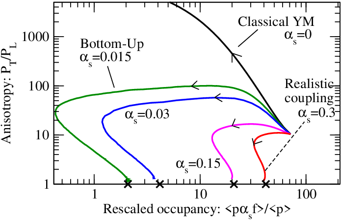
Fig. 4 displays the non-equilibrium evolution of a system within kinetic theory from [27]. The initial condition for the kinetic theory evolution is a parametrization of a CYM simulation at a switching time . The parametrisation is chosen to match energy density and with the classical simulation of [19] at . The figure contains trajectories from simulations with different values of the coupling constant . The x-axis is rescaled with such that for all values of , overoccupied initial condition with falls on the same point in the plane of occupancy and aniostropy. With such a rescaling, taking the limit keeping the initial fixed, gives a non-trivial limit that corresponds to the CYM. In terms of the figure, this limit corresponds to sending to infinitely far to the left, so that occupancies of order one are never reached in a simulation. This trajectory is labelled “classical YM”, and indeed what is seen is consistent with CYM simulations. The system becomes ever more dilute and anisotropic and never thermalizes.
For a small but non-zero , the kinetic theory simulation eventually reaches , and the qualitative change in the dynamics is clearly visible in the line labelled “Bottom-Up” in Fig. 4. When the occupancies become small, the EKT simulation deviates from the classical limit and the growth of the anisotropy stops. Eventually the EKT evolution brings the trajectory close to thermal equilibrium Fig. 4 as anticipated by [6] and consistent with expectation of Fig. 1.
Increasing the coupling further does not lead into further qualitative change. At larger couplings, the features in the trajectory arising from the scale separations provided by the weak coupling do become less pronounced and the system takes a somewhat more straightforward path to equilibrium.
4.1 Hydrodynamization
As the kinetic theory evolution brings the system close to thermal equilibrium, it should at late times be described by hydrodynamics. This is illustrated in Fig. 5, which depicts the time evolution of the components of the energy momentum tensor from a simulation with (left) and (right). The energy density and the transverse and longitudinal pressures and are normalized by . With this normalization, if the evolution is described by ideal hydrodynamics (with conformal equation of state ) for which , the lines should be horizontal and fall on top of each other. It can be clearly seen from the figure that indeed at late times, the lines asymptote to horizontal lines, and at late times the system is indeed described by ideal hydrodynamics.
According to the hydrodynamical theory, the approach to ideal hydrodynamics should be described by viscous hydrodynamics, which gives a prediction that depends only on the shear viscosity of the matter. As this is a well known quantity at weak coupling [24], the comparison with the parameter free prediction of hydrodynamics provides a very robust test. The prediction from viscous hydrodynamics is shown as the blue dashed line in Fig. 5. The approach is well captured by the hydrodynamical prediction for both couplings shown. For the small coupling , the viscous hydrodynamics agrees with the kinetic theory simulation at very late times . The simulation with intermediate coupling shows qualitatively similar features but differs quantitatively; it follows the hydrodynamical line already around . Converting this to physical units using a typical estimate of GeV gives hydrodynamization times of fm/c. It is quite remarkable that the hydrodynamical theory works already at this time, when the anisotropies are still quite large .
5 Discussions
In these proceedings I have discussed the not-so-straight-forward way the heavy-ion collisions thermalize, isotropize, and reach hydrodynamical flow in the limit of weak coupling. The system undergoes two smoothly connected stages before hydrodynamizing, the overoccupied and the underoccupied stages. These stages must be described in terms of different degrees of freedom, either in terms of classical fields or in terms of (semi-)classical particles. The thermalization times, obtained from the weak coupling framework extrapolated to intermediate couplings show agreement with the phenomenological expectation of 1fm/c.
The effective kinetic theory framework that describes the thermalization is used also to describe physics at widely different energy scales in the collision such as photon production and jet quenching. As such, the unifying kinetic theory prescription and the early time dynamics builds a bridge between the soft physics of flow and hard probes.
At present there are still several caveats that need to be ironed out before the model is ready for realistic phenomenology. So far the studies do not include fermions, which play a subleading role in the process of thermalization due to fermi statistics and color factors. However, the thermalization of fermions is crucial, for example, to electromagnetic probes, and if the chemical equilibration happens delayed with respect to kinematic thermalization, one could question whether the 2+1 flavour equation of state is the right EoS to use at early times in hydrodynamical simulations. The current implementation of the EKT does not allow for transverse dynamics, which is a crucial for the preflow, and the numerical role of certain plasma unstable modes is still somewhat unclear. Also, further work in the interface between the CYM and EKT is needed. However, while there are still several caveats, the list is getting shorter and the field of weak coupling thermalization is becoming a quantitative field.
How much of this theoretical exercise performed at the weak coupling limit carries through to physical heavy-ion collisions that are performed at RHIC or at the LHC, which unfortunately do not run at the asymptotic limit ? Are we allowed to extrapolate the weak coupling results to the relevant interesting intermediate couplings around ? A pessimist view would be to note that perturbation theory at finite temperature is notoriously badly convergent at temperatures close to [28]. However, an optimist would notice that as the thermalization takes place rather fast, the resulting temperatures at are still of order . This does lie in the temperature range where the perturbation theory in its modern incarnations seems to describe lattice results. The hydrodynamical evolution will eventually cool the system to a temperature range where a weak coupling description of the medium most likely is inappropriate, but by then the system has been already passed to a hydrodynamical description. As the hydrodynamical analysis mostly constrain the minimum of around [29], not its value around , this picture is not in contrast with the phenomenology and the paradigm of small .
So far the strategy has been to extrapolate the weak coupling results to intermediate couplings expected to realize in physical collisions. The same goes for the strong coupling studies where the results obtained at infinite coupling are again extrapolated down to intermediate couplings. However, perhaps a better strategy than extrapolating would be to use all available information to constrain the intermediate couplings; to interpolate rather than extrapolate. First steps in this direction are taken in [30], where non-equilibrium evolutions of strongly and weakly coupled theories with similar initial conditions are compared.
Whether the strategy is to extrapolate or to interpolate in coupling, it is clear that it is of importance to push the calculations beyond the leading order accuracy, both at weak and at strong coupling in order to increase precision of the results and to better evaluate at what range of couplings they provide useful constraints. While it will be a long way to NLO, there have been important advances in the recent past to this direction [31].
References
- [1] R. Baier, P. Romatschke, D. T. Son, A. O. Starinets, M. A. Stephanov, Relativistic viscous hydrodynamics, conformal invariance, and holography, JHEP 04 (2008) 100. arXiv:0712.2451, doi:10.1088/1126-6708/2008/04/100.
- [2] P. M. Chesler, L. G. Yaffe, Horizon formation and far-from-equilibrium isotropization in supersymmetric Yang-Mills plasma, Phys. Rev. Lett. 102 (2009) 211601. arXiv:0812.2053, doi:10.1103/PhysRevLett.102.211601.
- [3] P. M. Chesler, L. G. Yaffe, Holography and colliding gravitational shock waves in asymptotically spacetime, Phys. Rev. Lett. 106 (2011) 021601. arXiv:1011.3562, doi:10.1103/PhysRevLett.106.021601.
- [4] W. van der Schee, P. Romatschke, S. Pratt, Fully Dynamical Simulation of Central Nuclear Collisions, Phys. Rev. Lett. 111 (22) (2013) 222302. arXiv:1307.2539, doi:10.1103/PhysRevLett.111.222302.
- [5] F. Gelis, E. Iancu, J. Jalilian-Marian, R. Venugopalan, The Color Glass Condensate, Ann. Rev. Nucl. Part. Sci. 60 (2010) 463–489. arXiv:1002.0333, doi:10.1146/annurev.nucl.010909.083629.
- [6] R. Baier, A. H. Mueller, D. Schiff, D. T. Son, ’Bottom up’ thermalization in heavy ion collisions, Phys. Lett. B502 (2001) 51–58. arXiv:hep-ph/0009237, doi:10.1016/S0370-2693(01)00191-5.
- [7] A. Kurkela, G. D. Moore, Thermalization in Weakly Coupled Nonabelian Plasmas, JHEP 12 (2011) 044. arXiv:1107.5050, doi:10.1007/JHEP12(2011)044.
- [8] A. Kurkela, G. D. Moore, UV Cascade in Classical Yang-Mills Theory, Phys. Rev. D86 (2012) 056008. arXiv:1207.1663, doi:10.1103/PhysRevD.86.056008.
- [9] S. Schlichting, Turbulent thermalization of weakly coupled non-abelian plasmas, Phys. Rev. D86 (2012) 065008. arXiv:1207.1450, doi:10.1103/PhysRevD.86.065008.
- [10] A. Kurkela, E. Lu, Approach to Equilibrium in Weakly Coupled Non-Abelian Plasmas, Phys. Rev. Lett. 113 (18) (2014) 182301. arXiv:1405.6318, doi:10.1103/PhysRevLett.113.182301.
- [11] A. Kurkela, G. D. Moore, Bjorken Flow, Plasma Instabilities, and Thermalization, JHEP 11 (2011) 120. arXiv:1108.4684, doi:10.1007/JHEP11(2011)120.
- [12] A. H. Mueller, D. T. Son, On the Equivalence between the Boltzmann equation and classical field theory at large occupation numbers, Phys. Lett. B582 (2004) 279–287. arXiv:hep-ph/0212198, doi:10.1016/j.physletb.2003.12.047.
- [13] S. Jeon, The Boltzmann equation in classical and quantum field theory, Phys. Rev. C72 (2005) 014907. arXiv:hep-ph/0412121, doi:10.1103/PhysRevC.72.014907.
- [14] T. Epelbaum, F. Gelis, Pressure isotropization in high energy heavy ion collisions, Phys. Rev. Lett. 111 (2013) 232301. arXiv:1307.2214, doi:10.1103/PhysRevLett.111.232301.
- [15] J. Berges, K. Boguslavski, S. Schlichting, R. Venugopalan, Universal attractor in a highly occupied non-Abelian plasma, Phys. Rev. D89 (11) (2014) 114007. arXiv:1311.3005, doi:10.1103/PhysRevD.89.114007.
- [16] A. Krasnitz, R. Venugopalan, Nonperturbative computation of gluon minijet production in nuclear collisions at very high-energies, Nucl. Phys. B557 (1999) 237. arXiv:hep-ph/9809433, doi:10.1016/S0550-3213(99)00366-1.
- [17] A. Krasnitz, R. Venugopalan, The Initial energy density of gluons produced in very high-energy nuclear collisions, Phys. Rev. Lett. 84 (2000) 4309–4312. arXiv:hep-ph/9909203, doi:10.1103/PhysRevLett.84.4309.
- [18] T. Lappi, Production of gluons in the classical field model for heavy ion collisions, Phys. Rev. C67 (2003) 054903. arXiv:hep-ph/0303076, doi:10.1103/PhysRevC.67.054903.
- [19] T. Lappi, Gluon spectrum in the glasma from JIMWLK evolution, Phys. Lett. B703 (2011) 325–330. arXiv:1105.5511, doi:10.1016/j.physletb.2011.08.011.
- [20] J. Berges, K. Boguslavski, S. Schlichting, R. Venugopalan, Turbulent thermalization process in heavy-ion collisions at ultrarelativistic energies, Phys. Rev. D89 (7) (2014) 074011. arXiv:1303.5650, doi:10.1103/PhysRevD.89.074011.
- [21] L. D. McLerran, R. Venugopalan, Gluon distribution functions for very large nuclei at small transverse momentum, Phys. Rev. D49 (1994) 3352–3355. arXiv:hep-ph/9311205, doi:10.1103/PhysRevD.49.3352.
- [22] G. Chen, R. J. Fries, J. I. Kapusta, Y. Li, Early Time Dynamics of Gluon Fields in High Energy Nuclear Collisions, Phys. Rev. C92 (2015) 064912. arXiv:1507.03524, doi:10.1103/PhysRevC.92.064912.
- [23] P. B. Arnold, G. D. Moore, L. G. Yaffe, Effective kinetic theory for high temperature gauge theories, JHEP 01 (2003) 030. arXiv:hep-ph/0209353, doi:10.1088/1126-6708/2003/01/030.
- [24] P. B. Arnold, G. D. Moore, L. G. Yaffe, Transport coefficients in high temperature gauge theories. 2. Beyond leading log, JHEP 05 (2003) 051. arXiv:hep-ph/0302165, doi:10.1088/1126-6708/2003/05/051.
- [25] B. Schenke, C. Gale, S. Jeon, MARTINI: An Event generator for relativistic heavy-ion collisions, Phys. Rev. C80 (2009) 054913. arXiv:0909.2037, doi:10.1103/PhysRevC.80.054913.
- [26] M. C. Abraao York, A. Kurkela, E. Lu, G. D. Moore, UV cascade in classical Yang-Mills theory via kinetic theory, Phys. Rev. D89 (7) (2014) 074036. arXiv:1401.3751, doi:10.1103/PhysRevD.89.074036.
- [27] A. Kurkela, Y. Zhu, Isotropization and hydrodynamization in weakly coupled heavy-ion collisions, Phys. Rev. Lett. 115 (18) (2015) 182301. arXiv:1506.06647, doi:10.1103/PhysRevLett.115.182301.
- [28] K. Kajantie, M. Laine, K. Rummukainen, Y. Schroder, The Pressure of hot QCD up to g6 ln(1/g), Phys. Rev. D67 (2003) 105008. arXiv:hep-ph/0211321, doi:10.1103/PhysRevD.67.105008.
- [29] H. Niemi, K. J. Eskola, R. Paatelainen, Event-by-event fluctuations in perturbative QCD + saturation + hydro model: pinning down QCD matter shear viscosity in ultrarelativistic heavy-ion collisionsarXiv:1505.02677.
- [30] L. Keegan, A. Kurkela, P. Romatschke, W. van der Schee, Y. Zhu, Weak and strong coupling equilibration in nonabelian gauge theoriesarXiv:1512.05347.
- [31] J. Ghiglieri, G. D. Moore, D. Teaney, Jet-Medium Interactions at NLO in a Weakly-Coupled Quark-Gluon PlasmaarXiv:1509.07773.