Analysis of SDFEM on Shishkin triangular meshes and hybrid meshes for problems with characteristic layers Note: This research was partly supported by NSF of China ( Grant Nos. 11501335, 11401349 and 11501334) and NSF of Shandong Province (Grant Nos. BS2014SF008 and ZR2015FQ014).

Jin Zhang Corresponding author: Corresponding author: jinzhangalex@hotmail.com Address: School of Mathematical Sciences, Shandong Normal University, Jinan 250014, China Xiaowei Liu Note: Email: xwliuvivi@hotmail.com Address: College of Science, Qilu University of Technology, Jinan 250353, China.

Abstract

In this paper, we analyze the streamline diffusion finite element method (SDFEM) for a model singularly perturbed convection-diffusion equation on a Shishkin triangular mesh and hybrid meshes. Supercloseness property of $u^{I}-u^{N}$ is obtained, where $u^{I}$ is the interpolant of the solution $u$ and $u^{N}$ is the SDFEM’s solution. The analysis depends on novel integral inequalities for the diffusion and convection parts in the bilinear form. Furthermore, analysis on hybrid meshes shows that bilinear elements should be recommended for the exponential layer, not for the characteristic layer. Finally, numerical experiments support these theoretical results.

1 Introduction

We consider the singularly perturbed boundary value problem

\begin{array}[]{rcl}-\varepsilon\Delta u+bu_{x}+cu=f&\mbox{in}&\Omega=(0,1)^{2},\\ u=0&\mbox{on}&\partial\Omega,\end{array}

(1.1)

where $\varepsilon\ll|b|$ is a small positive parameter, the functions $b(x,y)$ , $c(x,y)$ and $f(x,y)$ are supposed sufficiently smooth. We also assume

b(x,y)\geq\beta>0,\,c(x,y)-\frac{1}{2}b_{x}(x,y)\geq\mu_{0}>0\quad\text{on $\bar{\Omega},$}

where $\beta$ and $\mu_{0}$ are some constants. The solution of (1.1) typically has an exponential layer of width $O(\varepsilon\ln(1/\varepsilon))$ near the outflow boundary at $x=1$ and two characteristic (or parabolic) layers of width $O(\sqrt{\varepsilon}\ln(1/\varepsilon))$ near the characteristic boundaries at $y=0$ and $y=1$ .

Because of the presence of layers, standard finite element methods suffer from nonphysical oscillations unless meshes are taken sufficiently fine which are useless for practical purposes. Thus, stabilized methods and/or a priori adapted meshes (see [15, 12]) are widely used in order to get discrete solutions with satisfactory stability and accuracy. Among them, the streamline diffusion finite element method (SDFEM) [7] combined with the Shishkin mesh [14] presents good numerical performances and has been widely studied, see [17, 5, 3, 18].

In this work, we will analyze supercloseness property of the SDFEM for problem (1.1). Here “supercloseness” means the convergence order of $u^{I}-u^{N}$ in some norm is greater than one of $u-u^{I}$ . This property in the case of rectangular meshes has been analyzed in [17, 5] by means of integral identities [10] and it is helpful to derive optimal $L^{2}$ estimates, $L^{\infty}$ bounds and postprocessing procedures. Unfortunately, on triangular meshes few results of supercloseness property could be found up to now. In this article, we present it in Theorem 4.1 by means of novel integral inequalities, i.e., Lemmas 3.1 and 3.2. Furthermore, the SDFEM is analyzed on Shishkin hybrid meshes which consist of rectangles and triangles. Theorem 5.1 shows that rectangles are strongly recommended for the exponential layer and not necessary for the characteristic layer.

Here is the outline of this article. In §2 we give some a priori information for the solution of (1.1), then introduce a Shishkin mesh and a streamline diffusion finite element method on the mesh. In §3 we present integral inequalities and the interpolation errors. In §4 we analyze the supercloseness property on the Shishkin triangular mesh. In §5 we obtain supercloseness property again on hybrid meshes. Finally, some numerical results are presented in §6.

Throughout the article, the standard notations for the Sobolev spaces and norms will be used; and generic constants $C$ , $C_{i}$ are independent of $\varepsilon$ and $N$ . An index will be attached to indicate an inner product or a norm on a subdomain $D$ , for example, $(\cdot,\cdot)_{D}$ and $\|\cdot\|_{D}$ .

2 Regularity results, Shishkin meshes and the SDFEM

2.1 Regularity results

As mentioned before the solution $u$ of (1.1) possesses an exponential layer at $x=1$ and two characteristic layers at $y=0$ and $y=1$ . For our later analysis we shall make the following assumption.

Assumption 2.1.

The solution $u$ of (1.1) can be decomposed as

	$u=S+E_{1}+E_{2}+E_{12},\quad\forall(x,y)\in\bar{\Omega}.$	(2.1a)
For $0\leq i+j\leq 3$ , the regular part satisfies
	$\left\|\frac{\partial^{i+j}S}{\partial x^{i}\partial y^{j}}(x,y)\right\|\leq C,$	(2.1b)
while for $0\leq i+j\leq 3$ , the layer terms satisfy
	$\left\|\frac{\partial^{i+j}E_{1}}{\partial x^{i}\partial y^{j}}(x,y)\right\|\leq C\varepsilon^{-i}e^{-\beta(1-x)/\varepsilon},$	(2.1c)
	$\left\|\frac{\partial^{i+j}E_{2}}{\partial x^{i}\partial y^{j}}(x,y)\right\|\leq C\varepsilon^{-j/2}(e^{-y/\sqrt{\varepsilon}}+e^{-(1-y)/\sqrt{\varepsilon}}),$	(2.1d)
and
	$\quad\quad\quad\left\|\frac{\partial^{i+j}E_{12}}{\partial x^{i}\partial y^{j}}(x,y)\right\|\leq C\varepsilon^{-(i+j/2)}e^{-\beta(1-x)/\varepsilon}(e^{-y/\sqrt{\varepsilon}}+e^{-(1-y)/\sqrt{\varepsilon}}).$	(2.1e)

Remark 2.1.

In [8, 9] Kellogg and Stynes presented sufficient compatibility conditions on $f$ for constant functions $b$ , $c$ that ensure the existence of (2.1a)–(2.1e).

2.2 Shishkin meshes

When discretizing (1.1), first we divide the domain $\Omega$ into four(six) subdomains as $\bar{\Omega}=\Omega_{s}\cup\Omega_{x}\cup\Omega_{y}\cup\Omega_{xy}$ (see Fig. 2), where

		$\displaystyle\Omega_{s}:=\left[0,1-\lambda_{x}\right]\times\left[\lambda_{y},1-\lambda_{y}\right],$		$\displaystyle\Omega_{y}:=\left[0,1-\lambda_{x}\right]\times\left(\left[0,\lambda_{y}\right]\cup\left[1-\lambda_{y},1\right]\right),$
		$\displaystyle\Omega_{x}:=\left[1-\lambda_{x},1\right]\times\left[\lambda_{y},1-\lambda_{y}\right],$		$\displaystyle\Omega_{xy}:=\left[1-\lambda_{x},1\right]\times\left(\left[0,\lambda_{y}\right]\cup\left[1-\lambda_{y},1\right]\right).$

Two parameters $\lambda_{x}$ and $\lambda_{y}$ are used here for mesh transition from coarse to fine and are defined by

\lambda_{x}:=\min\left\{\frac{1}{2},\rho\frac{\varepsilon}{\beta}\ln N\right\}\quad\mbox{and}\quad\lambda_{y}:=\min\left\{\frac{1}{4},\rho\sqrt{\varepsilon}\ln N\right\}.

For technical reasons, we set $\rho=2.5$ . Moreover, we assume $\varepsilon\leq\min\{N^{-1},\ln^{-6}N\}$ and

\lambda_{x}=\rho\varepsilon\beta^{-1}\ln N\leq\frac{1}{2}\quad\text{and}\quad\lambda_{y}=\rho\sqrt{\varepsilon}\ln N\leq\frac{1}{4}

as is typically the case for (1.1).

Refer to caption — Fig.1: Dissection of $\Omega$ and triangulation $\mathcal{T}_{N}$ .

Next, we introduce the set of mesh points $\left\{(x_{i},y_{j})\in\bar{\Omega}:\;i,\,j=0,\,\cdots,\,N\right\}$ defined by

	$\displaystyle x_{i}=$	$\displaystyle 2i(1-\lambda_{x})/N,$	for $i=0,\,\cdots,\,N/2$ ,
	$\displaystyle x_{i}=$	$\displaystyle 1-2(N-i)\lambda_{x}/N,$	for $i=N/2+1,\,\cdots,\,N$

and

$\displaystyle y_{j}=$	$\displaystyle 3j\lambda_{y}/N,$	for $j=0,\,\cdots,\,N/3$ ,
$\displaystyle y_{j}=$	$\displaystyle(3j/N-1)-3(2j-N)\lambda_{y}/N,$	for $j=N/3+1,\,\cdots,\,2N/3$ ,
$\displaystyle y_{j}=$	$\displaystyle 1-3(N-j)\lambda_{y}/N,$	for $j=2N/3+1,\,\cdots,\,N$ .

By drawing lines through these mesh points parallel to the $x$ -axis and $y$ -axis, the domain $\Omega$ is partitioned into rectangles and triangles by drawing the diagonal in each rectangle (see Fig. 2). This yields a piecewise uniform triangulation of $\Omega$ denoted by $\mathcal{T}_{N}$ .

We define $h_{x,i}:=x_{i+1}-x_{i}$ and $h_{y,j}:=y_{j+1}-y_{j}$ which satisfy

	$\displaystyle N^{-1}\leq$	$\displaystyle h_{x,i}=:H_{x},h_{y,j}=:H_{y}\leq 3N^{-1},\quad 0\leq i<N/2,\;N/3\leq j<2N/3,$
	$\displaystyle C_{1}\varepsilon N^{-1}\ln N$	$\displaystyle\leq h_{x,i}=:h_{x}\leq C_{2}\varepsilon N^{-1}\ln N,\quad N/2\leq i<N,$
	$\displaystyle C_{1}\sqrt{\varepsilon}N^{-1}\ln N$	$\displaystyle\leq h_{y,j}=:h_{y}\leq C_{2}\sqrt{\varepsilon}N^{-1}\ln N,\quad j=0,\ldots,N/3-1;\;2N/3,\ldots,N-1.$

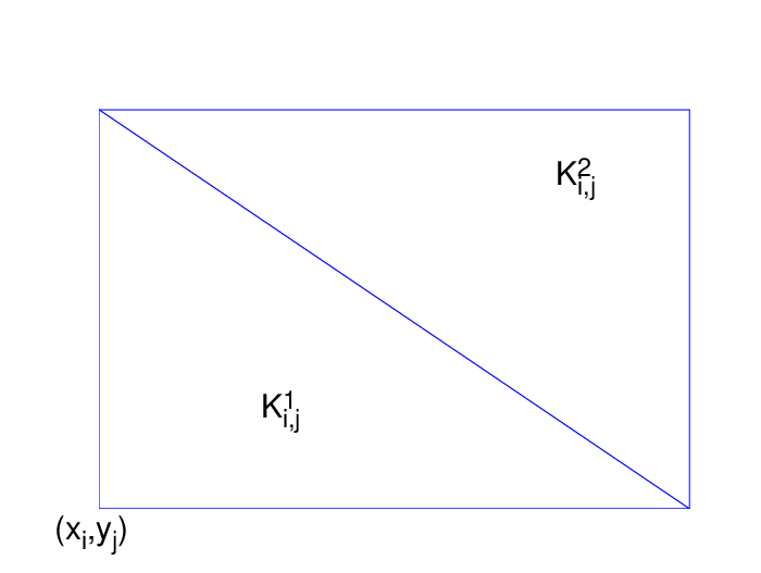
For mesh elements we shall use some notations: $K^{1}_{i,j}$ for the mesh triangle with vertices $(x_{i},y_{j})$ , $(x_{i+1},y_{j})$ and $(x_{i},y_{j+1})$ ; $K^{2}_{i,j}$ for the mesh triangle with vertices $(x_{i},y_{j+1})$ , $(x_{i+1},y_{j})$ and $(x_{i+1},y_{j+1})$ (see Fig. 2); $K$ for a generic mesh triangle.

2.3 The streamline diffusion finite element method

The variational formulation of problem (1.1) is:

\left\{\begin{array}[]{lr}\text{Find $u\in V$ such that for all $v\in V$}\\ \varepsilon(\nabla u,\nabla v)+(bu_{x}+cu,v)=(f,v),\end{array}\right.

(2.2)

where $V:=H^{1}_{0}(\Omega)$ . Note that the weak formulation (2.2) has a unique solution by means of the Lax-Milgram Lemma.

Let $V^{N}\subset V$ be the finite element space of piecewise linear elements on the Shishkin mesh $\mathcal{T_{N}}$ . The SDFEM consists in adding weighted residuals to the standard Galerkin method in order to stabilize the discretization. It reads:

\left\{\begin{array}[]{lr}\text{Find $u^{N}\in V^{N}$ such that for all $v^{N}\in V^{N}$},\\ a_{SD}(u^{N},v^{N})=(f,v^{N})+\underset{K\subset\Omega}{\sum}(f,\delta_{K}bv^{N}_{x})_{K},\end{array}\right.

(2.3)

where

a_{SD}(u^{N},v^{N})=a_{Gal}(u^{N},v^{N})+a_{stab}(u^{N},v^{N})

and

	$\displaystyle a_{Gal}(u^{N},v^{N})$	$\displaystyle=\varepsilon(\nabla u^{N},\nabla v^{N})+(bu^{N}_{x}+cu^{N},v^{N}),$
	$\displaystyle a_{stab}(u^{N},v^{N})$	$\displaystyle=\sum_{K\subset\Omega}(-\varepsilon\Delta u^{N}+bu^{N}_{x}+cu^{N},\delta_{K}bv^{N}_{x})_{K}.$

Note that $\Delta u^{N}=0$ in $K$ for $u^{N}|_{K}\in P_{1}(K)$ and $\delta_{K}=\delta(x,y)|_{K}$ . In this article, the stabilization parameter $\delta$ is chosen to be constant on each subdomain of $\Omega$ . Denote by $\delta_{s}$ the restriction of $\delta$ in $\Omega_{s}$ and similar $\delta_{x}$ , $\delta_{y}$ and $\delta_{xy}$ .

The SDFEM satisfies the following orthogonality

a_{SD}(u-u^{N},v^{N})=0,\quad\forall v^{N}\in V^{N}.

(2.4)

Moreover, as shown in [12], if the stabilization parameter satisfies

0\leq\delta_{K}\leq\frac{\mu_{0}}{2\|c\|^{2}_{L^{\infty}(K)}},

(2.5)

the SDFEM is coercive with respect to the streamline diffusion norm

a_{SD}(v^{N},v^{N})\geq\frac{1}{2}\|v^{N}\|^{2}_{SD},\quad\forall v^{N}\in V^{N}

(2.6)

where

\|v^{N}\|^{2}_{SD}:=\|v^{N}\|^{2}_{\varepsilon}+\sum_{K\subset\Omega}\delta_{K}\|bv^{N}_{x}\|^{2}_{K}

(2.7)

and $\|v^{N}\|^{2}_{\varepsilon}:=\varepsilon|v^{N}|^{2}_{1}+\mu_{0}\|v^{N}\|^{2}$ . Note that existence and uniqueness of the solution to (2.3) is guaranteed by the coercivity (2.6).

3 Integral inequalities and interpolation errors

In this section we present integral inequalities for the diffusion and convection parts in the bilinear form and some interpolation bounds for our later analysis. For notation convenience, we set

\partial^{l}_{x}\partial^{m}_{y}v:=\frac{\partial^{l+m}v}{\partial x^{l}\partial y^{m}}.

The following lemma will be used to obtain sharp estimates of the diffusion part in the bilinear form $a_{SD}(\cdot,\cdot)$ .

Lemma 3.1.

Assume that $w\in C^{3}(\bar{\Omega})$ and $v^{N}\in V^{N}$ . Let $w^{I}$ be the standard nodal linear interpolation on $\mathcal{T}_{N}$ and $l$ , $m$ be nonnegative integers. If $h_{y,j-1}=h_{y,j}$ , then we have

\left|\int_{\mathcal{Q}_{i,j}}(w-w^{I})_{x}v^{N}_{x}\mathrm{d}x\mathrm{d}y\right|\leq C\sum_{l+m=2}h^{l}_{x,i}h^{m}_{y,j}\|\partial^{l+1}_{x}\partial^{m}_{y}w\|_{L^{\infty}(\mathcal{Q}_{i,j})}\|v^{N}_{x}\|_{L^{1}(\mathcal{Q}_{i,j})},

where $\mathcal{Q}_{i,j}:=K^{1}_{i,j}\cup K^{2}_{i,j-1}$ . If $h_{x,i-1}=h_{x,i}$ , then we have

\left|\int_{\mathcal{S}_{i,j}}(w-w^{I})_{y}v^{N}_{y}\mathrm{d}x\mathrm{d}y\right|\leq C\sum_{l+m=2}h^{l}_{x,i}h^{m}_{y,j}\|\partial^{l}_{x}\partial^{m+1}_{y}w\|_{L^{\infty}(\mathcal{S}_{i,j})}\|v^{N}_{y}\|_{L^{1}(\mathcal{S}_{i,j})}

where $\mathcal{S}_{i,j}:=K^{2}_{i-1,j}\cup K^{1}_{i,j}$ .

Proof.

Note that $v^{N}_{x}$ is a constant on the set $\mathcal{Q}_{i,j}$ . First we expand $(w-w^{I})_{x}$ by Taylor’s formula at $(x_{i},y_{j})$ with Lagrange form of the remainder. After integration on $\mathcal{Q}_{i,j}$ , we can offset terms involving low derivatives of $w$ . Then the first inequality is obtained. The second inequality can be proved similarly . See [19, Lemma 2.1] for more details. ∎

The following integral inequalities provide sharp estimates of the convection part in the bilinear form $a_{SD}(\cdot,\cdot)$ .

Lemma 3.2.

Assume that $w\in C^{3}(\bar{\Omega})$ and let $w^{I}$ be the piecewise linear interpolation of $w$ on $\mathcal{T}_{N}$ . Set $\alpha=1$ or $\alpha=2$ and $p,q,l,m$ are nonnegative integers satisfying $0\leq p+q\leq 1$ . Suppose $h_{x,i-1}=h_{x,i}$ , then we have

		$\displaystyle\left\|\int_{K^{\alpha}_{i-1,j}}\partial^{p}_{x}\partial^{q}_{y}(w-w^{I})\mathrm{d}x\mathrm{d}y-\int_{K^{\alpha}_{i,j}}\partial^{p}_{x}\partial^{q}_{y}(w-w^{I})\mathrm{d}x\mathrm{d}y\right\|$		(3.1)
	$\displaystyle\leq$	$\displaystyle C\sum_{l+m=3}h^{l+1-p}_{x,i}h^{m+1-q}_{y,j}\left\\|\partial^{l}_{x}\partial^{m}_{y}w\right\\|_{L^{\infty}(K^{\alpha}_{i-1,j}\cup K^{\alpha}_{i,j})}.$

Suppose $h_{y,j-1}=h_{y,j}$ , then we have

		$\displaystyle\left\|\int_{K^{\alpha}_{i,j-1}}\partial^{p}_{x}\partial^{q}_{y}(w-w^{I})\mathrm{d}x\mathrm{d}y-\int_{K^{\alpha}_{i,j}}\partial^{p}_{x}\partial^{q}_{y}(w-w^{I})\mathrm{d}x\mathrm{d}y\right\|$		(3.2)
	$\displaystyle\leq$	$\displaystyle C\sum_{l+m=3}h^{l+1-p}_{x,i}h^{m+1-q}_{y,j}\left\\|\partial^{l}_{x}\partial^{m}_{y}w\right\\|_{L^{\infty}(K^{\alpha}_{i,j-1}\cup K^{\alpha}_{i,j})}.$

Proof.

We just prove (3.1) for $\alpha=1$ and $p=q=0$ . The other estimates can be obtained similarly.

Expanding $(w-w^{I})_{x}$ by Taylor’s formula at $(x_{i},y_{j})$ , we have

		$\displaystyle(w-w^{I})\|_{K^{1}_{i,j}}=w(x,y)-(w(x_{i},y_{j})\lambda_{1}+w(x_{i+1},y_{j})\lambda_{2}+w(x_{i},y_{j+1})\lambda_{3})$
		$\displaystyle=w(x_{i},y_{j})+\left(w_{x}(x_{i},y_{j})(x-x_{i})+w_{y}(x_{i},y_{j})(y-y_{j})\right)$
		$\displaystyle+\left(w_{xx}(x_{i},y_{j})\frac{(x-x_{i})^{2}}{2}+w_{xy}(x_{i},y_{j})(x-x_{i})(y-y_{j})+w_{yy}(x_{i},y_{j})\frac{(y-y_{j})^{2}}{2}\right)$
		$\displaystyle-\left(w(x_{i},y_{j})+w_{x}(x_{i},y_{j})h_{x,i}\lambda_{2}+w_{y}(x_{i},y_{j})h_{y,j}\lambda_{3}\right)$
		$\displaystyle-\left(w_{xx}(x_{i},y_{j})\frac{h^{2}_{x,i}}{2}\lambda_{2}+w_{yy}(x_{i},y_{j})\frac{h^{2}_{y,j}}{2}\lambda_{3}\right)+\mathcal{R}_{i,j},$

where $\lambda_{1}=1-\lambda_{2}-\lambda_{3}$ , $\lambda_{2}=\frac{x-x_{i}}{h_{x,i}}$ , $\lambda_{3}=\frac{y-y_{j}}{h_{y,j}}$ are the area basis functions and

\|\mathcal{R}_{i,j}\|_{L^{\infty}(K^{1}_{i,j})}\leq C\sum_{l+m=3}h^{l}_{x,i}h^{m}_{y,j}\left\|\partial^{l}_{x}\partial^{m}_{y}w\right\|_{L^{\infty}(K^{1}_{i,j})}.

(3.3)

Direct calculations yield

	$\displaystyle\int_{K^{1}_{i,j}}(w-w^{I})\mathrm{d}x\mathrm{d}y=$	$\displaystyle w_{xx}(x_{i},y_{j})\left(-\frac{h^{3}_{x,i}h_{y,j}}{24}\right)+w_{xy}(x_{i},y_{j})\left(\frac{h^{2}_{x,i}h^{2}_{y,j}}{24}\right)$		(3.4)
		$\displaystyle+w_{yy}(x_{i},y_{j})\left(-\frac{h_{x,i}h^{3}_{y,j}}{24}\right)+\int_{K^{1}_{i,j}}\mathcal{R}_{i,j}\mathrm{d}x\mathrm{d}y.$

Similarly, we have

	$\displaystyle\int_{K^{1}_{i-1,j}}(w-w^{I})\mathrm{d}x\mathrm{d}y=$	$\displaystyle w_{xx}(x_{i},y_{j})\left(-\frac{h^{3}_{x,i}h_{y,j}}{24}\right)+w_{xy}(x_{i},y_{j})\left(\frac{h^{2}_{x,i}h^{2}_{y,j}}{24}\right)$		(3.5)
		$\displaystyle+w_{yy}(x_{i},y_{j})\left(-\frac{h_{x,i}h^{3}_{y,j}}{24}\right)+\int_{K^{1}_{i-1,j}}\mathcal{R}_{i-1,j}\mathrm{d}x\mathrm{d}y$

and

\|\mathcal{R}_{i-1,j}\|_{L^{\infty}(K^{1}_{i-1,j})}\leq\sum_{l+m=3}h^{l}_{x,i}h^{m}_{y,j}\left\|\partial^{l}_{x}\partial^{m}_{y}w\right\|_{L^{\infty}(K^{1}_{i-1,j})}

(3.6)

where the condition $h_{x,i-1}=h_{x,i}$ has been used in (3.5).

Combining (3.3)—(3.6), we obtain (3.1) for $\alpha=1$ and $p=q=0$ . ∎

For analysis on Shishkin meshes, we need the following anisotropic interpolation error bounds given in [6, Lemma 3.2].

Lemma 3.3.

Let $K\in\mathcal{T}_{N}$ and $p\in(1,\infty]$ and suppose that $K$ is $K^{1}_{i,j}$ or $K^{2}_{i,j}$ . Assume that $w\in W^{2,p}(\Omega)$ and denote by $w^{I}$ the linear function that interpolates to $w$ at the vertices of $K$ . Then

		$\displaystyle\\|w-w^{I}\\|_{L^{p}(K)}\leq C\sum_{l+m=2}h^{l}_{x,i}h^{m}_{y,j}\\|\partial^{l}_{x}\partial^{m}_{y}w\\|_{L^{p}(K)},$
		$\displaystyle\\|(w-w^{I})_{x}\\|_{L^{p}(K)}\leq C\sum_{l+m=1}h^{l}_{x,i}h^{m}_{y,j}\\|\partial^{l+1}_{x}\partial^{m}_{y}w\\|_{L^{p}(K)},$
		$\displaystyle\\|(w-w^{I})_{y}\\|_{L^{p}(K)}\leq C\sum_{l+m=1}h^{l}_{x,i}h^{m}_{y,j}\\|\partial^{l}_{x}\partial^{m+1}_{y}w\\|_{L^{p}(K)},$

where $l$ and $m$ are nonnegative integers.

The following local estimates will also be frequently used.

Lemma 3.4.

Let $u^{I}$ and $E^{I}$ denote the piecewise linear interpolation of $u$ and $E$ , respectively, on the Shishkin mesh $\mathcal{T}_{N}$ , where $E$ can be any one of $E_{1}$ , $E_{2}$ or $E_{12}$ . Suppose that $u$ satisfies Assumption 2.1, then

		$\displaystyle\\|u-u^{I}\\|_{L^{\infty}(K)}\leq\left\{\begin{array}[]{ll}CN^{-2},&\text{if $K\subset\Omega_{s}$}\\ CN^{-2}\ln^{2}N,&\text{otherwise}\end{array}\right.,$
		$\displaystyle\\|E^{I}\\|_{L^{\infty}(\Omega_{s})}+\\|\nabla E^{I}\\|_{L^{1}(\Omega_{s})}\leq CN^{-\rho},$
		$\displaystyle\\|E^{I}_{1}\\|_{L^{\infty}(\Omega_{y})}+\\|E^{I}_{12}\\|_{L^{\infty}(\Omega_{y})}\leq CN^{-\rho},$
		$\displaystyle\\|(E^{I}_{12})_{y}\\|_{L^{1}(\Omega_{y})}\leq CN^{-(1+\rho)},$
		$\displaystyle\\|\nabla E^{I}_{1}\\|_{L^{1}(\Omega_{y})}+\\|(E^{I}_{12})_{x}\\|_{L^{1}(\Omega_{y})}\leq C\varepsilon^{1/2}N^{-\rho}\ln N.$

Proof.

The first inequality can be obtained in a similar way as [16, Theorem 4.2]. Here we only prove the second inequality for $E=E_{1}$ and the others can be proved similarly. Recalling $E^{I}_{1}$ is the piecewise linear interpolation of $E_{1}$ , we have

\|E^{I}_{1}\|_{L^{\infty}(\Omega_{s})}\leq\|E_{1}\|_{L^{\infty}(\Omega_{s})}\leq CN^{-\rho}

(3.7)

and

\displaystyle(E^{I}_{1})_{y}|_{K^{1}_{i,j}}

\displaystyle=\frac{E_{1}(x_{i},y_{j+1})-E_{1}(x_{i},y_{j})}{h_{y,j}}=(E_{1})_{y}(x_{i},\eta_{j})

where $\eta_{j}\in(y_{j},y_{j+1})$ . Similarly, we have $(E^{I}_{1})_{y}|_{K^{2}_{i,j}}=(E_{1})_{y}(x_{i+1},\tilde{\eta}_{j})$ with $\tilde{\eta}_{j}\in(y_{j},y_{j+1})$ and

(E^{I}_{1})_{x}|_{K^{1}_{i,j}}=(E_{1})_{x}(\xi_{i},y_{j}),\quad(E^{I}_{1})_{x}|_{K^{2}_{i,j}}=(E_{1})_{x}(\tilde{\xi}_{i},y_{j+1})

(3.8)

where $\xi_{i},\tilde{\xi}_{i}\in(x_{i},x_{i+1})$ . Recalling Assumption 2.1, we obtain

\displaystyle\left|(E^{I}_{1})_{y}|_{K}\right|\leq C\|(E_{1})_{y}\|_{L^{\infty}(\Omega_{s})}\leq CN^{-\rho},\;\forall K\subset\Omega_{s}.

Then we have

\|(E^{I}_{1})_{y}\|_{L^{1}(\Omega_{s})}\leq CN^{-\rho}.

(3.9)

Setting $\Omega_{s,r}:=\cup_{j=N/3}^{2N/3-2}\cup_{m=1}^{2}K^{m}_{N/2-1,j}$ . Recalling (3.8) and Assumption 2.1, we obtain

$\displaystyle\\|(E^{I}_{1})_{x}\\|_{L^{1}(\Omega_{s}\setminus\Omega_{s,r})}$	$\displaystyle=\sum_{i=0}^{N/2-2}\sum_{j=N/3}^{2N/3-1}\sum_{m=1}^{2}\\|(E^{I}_{1})_{x}\\|_{L^{1}(K^{m}_{i,j})}$	(3.10)
	$\displaystyle\leq C\sum_{i=0}^{N/2-2}N^{-1}\varepsilon^{-1}e^{-\beta(1-x_{i+1})/\varepsilon}$
	$\displaystyle\leq C\sum_{i=0}^{N/2-2}\int_{x_{i}}^{x_{i+1}}\varepsilon^{-1}e^{-\beta(1-x)/\varepsilon}\mathrm{d}x$
	$\displaystyle\leq C\int_{x_{0}}^{x_{N/2}}\varepsilon^{-1}e^{-\beta(1-x)/\varepsilon}\mathrm{d}x\leq CN^{-\rho}.$

Note that $\mathrm{meas}(\Omega_{s,r})\leq CN^{-1}$ , then we have

$\displaystyle\\|(E^{I}_{1})_{x}\\|_{L^{1}(\Omega_{s,r})}$	$\displaystyle\leq CN\\|E^{I}_{1}\\|_{L^{1}(\Omega_{s,r})}$	(3.11)
	$\displaystyle\leq CN\\|E^{I}_{1}\\|_{L^{\infty}(\Omega_{s,r})}\mathrm{meas}(\Omega_{s,r})$
	$\displaystyle\leq CN^{-\rho}$

where inverse estimates [2, Theorem 3.2.6] have been used.

Now collecting (3.7), (3.9), (3.10) and (3.11), we prove the inequality $\|E^{I}_{1}\|_{L^{\infty}(\Omega_{s})}+\|\nabla E^{I}_{1}\|_{L^{1}(\Omega_{s})}\leq CN^{-\rho}$ . ∎

4 Supercloseness property on triangular meshes

In this section, we will estimate each term in $a_{SD}(u-u^{I},v^{N})$ to derive the bound of $\|u^{I}-u^{N}\|_{SD}$ on the Shishkin triangular mesh $\mathcal{T}_{N}$ .

Lemma 4.1.

Let $u$ be the solution of (1.1) that satisfies Assumption 2.1, and $u^{I}\in V^{N}$ be the linear interpolation of $u$ on the Shishkin mesh. Then for all $v^{N}\in V^{N}$ , we have

\left|\varepsilon(\nabla(u-u^{I}),\nabla v^{N})\right|\leq C(\varepsilon^{1/4}N^{-3/2}+N^{-3/2})\ln^{3/2}N\;\|v^{N}\|_{SD}.

Proof.

Recalling the decomposition (2.1a), we set $E=E_{1}+E_{2}+E_{12}$ . Then we have

(\nabla(u-u^{I}),\nabla v^{N})=\mathrm{I}+\mathrm{II}+\mathrm{III},

where

	$\displaystyle\mathrm{I}:=$	$\displaystyle\left(\nabla(E_{2}-E^{I}_{2}),\nabla v^{N}\right)_{\Omega_{y}}+\left(\nabla(E-E^{I}),\nabla v^{N}\right)_{\Omega_{xy}}+\left(\nabla(S-S^{I}),\nabla v^{N}\right)_{\Omega_{s}\cup\Omega_{y}},$
	$\displaystyle\mathrm{II}:=$	$\displaystyle\left(\nabla(E-E^{I}),\nabla v^{N}\right)_{\Omega_{s}}+\left(\nabla(E_{1}-E^{I}_{1}),\nabla v^{N}\right)_{\Omega_{y}}+\left(\nabla(S-S^{I}),\nabla v^{N}\right)_{\Omega_{xy}}$
		$\displaystyle+\left(\nabla(E_{12}-E^{I}_{12}),\nabla v^{N}\right)_{\Omega_{y}},$
	$\displaystyle\mathrm{III}:=$	$\displaystyle\left(\nabla(S-S^{I}),\nabla v^{N}\right)_{\Omega_{x}}+\left((E_{1}-E^{I}_{1})_{y},v^{N}_{y}\right)_{\Omega_{x}}+\left(\nabla(E_{2}-E^{I}_{2}),\nabla v^{N}\right)_{\Omega_{x}}$
		$\displaystyle+\left(\nabla(E_{12}-E^{I}_{12}),\nabla v^{N}\right)_{\Omega_{x}}+\left((E_{1}-E^{I}_{1})_{x},v^{N}_{x}\right)_{\Omega_{x}}$
	$\displaystyle=:$	$\displaystyle\mathrm{III}_{1}+\ldots+\mathrm{III}_{4}+\mathrm{III}_{5}.$

The estimates of $\mathrm{I}$ depend on Lemma 3.1. Here we just present the detailed analysis for $((E_{2}-E^{I}_{2})_{y},v^{N}_{y})_{\Omega_{y}^{d}}$ where $\Omega_{y}^{d}:=[0,1-\lambda_{x}]\times[0,\lambda_{y}]$ , since the other terms can be analyzed in a similar way. First, we have

	$\displaystyle((E_{2}-E^{I}_{2})_{y},v^{N}_{y})_{\Omega_{y}^{d}}$	$\displaystyle=\sum_{i=0}^{N/2-1}\sum_{j=0}^{N/3-1}\sum_{m=1}^{2}((E_{2}-E^{I}_{2})_{y},v^{N}_{y})_{K^{m}_{i,j}}$
		$\displaystyle=\sum_{j=0}^{N/3-1}((E_{2}-E^{I}_{2})_{y},v^{N}_{y})_{K^{1}_{0,j}}+\sum_{j=0}^{N/3-1}((E_{2}-E^{I}_{2})_{y},v^{N}_{y})_{K^{2}_{N/2-1,j}}$
		$\displaystyle\;\;\;+\sum_{i=1}^{N/2-1}\sum_{j=0}^{N/3-1}((E_{2}-E^{I}_{2})_{y},v^{N}_{y})_{K^{2}_{i-1,j}\cup K^{1}_{i,j}}$
		$\displaystyle=:\mathrm{T}_{1}+\mathrm{T}_{2}+\mathrm{T}_{3}.$

Considering $v^{N}|_{\partial\Omega}=0$ , we have

\mathrm{T}_{1}=0.

(4.1)

Hölder inequalities and Lemma 3.3 yield

$\displaystyle\|\mathrm{T}_{2}\|$	$\displaystyle\leq C\\|(E_{2}-E^{I}_{2})_{y}\\|_{L^{\infty}(\Omega_{y,r})}\cdot\\|v^{N}_{y}\\|_{L^{1}(\Omega_{y,r})}$	(4.2)
	$\displaystyle\leq C\varepsilon^{-1/2}N^{-1}\ln N\cdot\varepsilon^{1/4}N^{-1/2}\ln^{1/2}N\\|v^{N}_{y}\\|_{\Omega_{y}}$
	$\displaystyle\leq C\varepsilon^{-3/4}N^{-3/2}\ln^{3/2}N\cdot\varepsilon^{1/2}\\|v^{N}_{y}\\|_{\Omega_{y}},$

where $\Omega_{y,r}=\bigcup_{j=0}^{N/3-1}K_{N/2-1,j}^{2}$ and we have used $\mathrm{meas}(\Omega_{y,r})\leq C\varepsilon^{1/2}N^{-1}\ln N$ . Using Lemma 3.1, we obtain

$\displaystyle\|\mathrm{T}_{3}\|$	$\displaystyle\leq C\varepsilon^{-1/2}N^{-2}\ln^{2}N\cdot\\|v^{N}_{y}\\|_{L^{1}(\Omega_{y}^{d})}$	(4.3)
	$\displaystyle\leq C\varepsilon^{-1/2}N^{-2}\ln^{2}N\cdot\varepsilon^{1/4}\ln^{1/2}N\\|v^{N}_{y}\\|_{\Omega_{y}}$
	$\displaystyle\leq C\varepsilon^{-3/4}N^{-2}\ln^{5/2}N\cdot\varepsilon^{1/2}\\|v^{N}_{y}\\|_{\Omega_{y}}.$

From (4.1)—(4.3), we obtain

|((E_{2}-E^{I}_{2})_{y},v^{N}_{y})_{\Omega_{y}}|\leq C\varepsilon^{-3/4}N^{-3/2}\ln^{3/2}N\;\|v^{N}\|_{SD}.

Similarly, we can estimate the remained terms in $\mathrm{I}$ and obtain

|\mathrm{I}|\leq C\varepsilon^{-3/4}N^{-3/2}\ln^{3/2}N\;\|v^{N}\|_{SD}.

(4.4)

Analysis of $\mathrm{II}$ depends on Lemmas 3.3, 3.4 and/or smallness of layer functions and layer domains. For example, inverse estimates [2, Theorem 3.2.6] and Lemma 3.4 yield

	$\displaystyle\|\left(\nabla(E-E^{I}),\nabla v^{N}\right)_{\Omega_{s}}\|\leq$	$\displaystyle\\|\nabla(E-E^{I})\\|_{L^{1}(\Omega_{s})}\\|\nabla v^{N}\\|_{L^{\infty}(\Omega_{s})}$
	$\displaystyle\leq$	$\displaystyle CN^{-\rho}\cdot N\\|\nabla v^{N}\\|_{\Omega_{s}}$
	$\displaystyle\leq$	$\displaystyle C\varepsilon^{-1/2}N^{1-\rho}\\|v^{N}\\|_{SD}.$

Thus we obtain

|\mathrm{II}|\leq C(\varepsilon^{-1/2}+\varepsilon^{-1/4}\ln^{1/2}N+\varepsilon^{-3/4}N^{-1}\ln^{1/2}N)N^{1-\rho}\|v^{N}\|_{SD}.

(4.5)

The analysis of $\mathrm{III}_{1}$ – $\mathrm{III}_{4}$ is similar to one of $\mathrm{II}$ and the estimate of $\mathrm{III}_{5}$ is similar to one of $\mathrm{I}$ . Thus we have

		$\displaystyle\|\mathrm{III}_{1}\|+\ldots+\|\mathrm{III}_{4}\|\leq C(N^{-1}\ln^{3/2}N+\varepsilon^{-1}N^{-\rho}\ln^{1/2}N)\\|v^{N}\\|_{SD},$		(4.6)
		$\displaystyle\|\mathrm{III}_{5}\|\leq C\varepsilon^{-1}N^{-3/2}\ln^{3/2}N\\|v^{N}\\|_{SD}.$		(4.7)

Collecting (4.4)–(4.7), the proof is done. ∎

Lemma 4.2.

Let $u$ be the solution of (1.1) that satisfies Assumption 2.1, and $u^{I}\in V^{N}$ be the linear interpolation of $u$ on the Shishkin mesh. Then for all $v^{N}\in V^{N}$ , we have

\left|(b(u-u^{I})_{x}+c(u-u^{I}),v^{N})\right|\leq C(A_{s}+A_{y}+(1+\varepsilon^{1/4}\ln N)N^{-2}\ln^{5/2}N)\|v^{N}\|_{SD},

(4.8)

where

\displaystyle A_{s}:=\min\{N^{-\rho}\delta_{s}^{-1/2},N^{1-\rho}\},A_{y}:=\varepsilon^{1/4}\min\{N^{-\rho}\delta_{y}^{-1/2},N^{1-\rho}\}\ln^{1/2}N.

Proof.

Integration by parts yields

\displaystyle(b(u-u^{I})_{x}+c(u-u^{I}),v^{N})

\displaystyle=-(b(u-u^{I}),v^{N}_{x})+((c-b_{x})(u-u^{I}),v^{N}).

Lemma 3.4 yields

|((c-b_{x})(u-u^{I}),v^{N})|\leq CN^{-2}\ln^{2}N\|v^{N}\|\leq CN^{-2}\ln^{2}N\|v^{N}\|_{SD}.

(4.9)

Recalling the decomposition (2.1a) and setting $E=E_{1}+E_{2}+E_{12}$ , we have

(b(u-u^{I}),v^{N}_{x})=\mathcal{I}+\mathcal{II},

where

	$\displaystyle\mathcal{I}:=$	$\displaystyle(b(E-E^{I}),v^{N}_{x})_{\Omega_{s}}+(b(u-u^{I}),v^{N}_{x})_{\Omega_{x}\cup\Omega_{xy}}$
		$\displaystyle+(b(E_{1}+E_{12}-(E^{I}_{1}+E^{I}_{12}),v^{N}_{x})_{\Omega_{y}},$
	$\displaystyle\mathcal{II}:=$	$\displaystyle(b(S-S^{I}),v^{N}_{x})_{\Omega_{s}}+(b(S-S^{I}),v^{N}_{x})_{\Omega_{y}}+(b(E_{2}-E^{I}_{2}),v^{N}_{x})_{\Omega_{y}}.$

The analysis of $\mathcal{I}$ is similar to one of $\mathrm{II}$ in Lemma 4.1. For example,

	$\displaystyle\|(b(E-E^{I}),v^{N}_{x})_{\Omega_{s}}\|$	$\displaystyle\leq CN^{-\rho}\\|v^{N}_{x}\\|_{L^{1}(\Omega_{s})}\leq CN^{-\rho}\\|v^{N}_{x}\\|_{\Omega_{s}}$
		$\displaystyle\leq\left\{\begin{array}[]{l}CN^{-\rho}\delta_{s}^{-1/2}\cdot\delta^{1/2}_{s}\\|v^{N}_{x}\\|_{\Omega_{s}}\\ CN^{1-\rho}\cdot\\|v^{N}\\|_{\Omega_{s}}\end{array}\right..$

Thus, we have

|\mathcal{I}|\leq C(A_{s}+A_{y}+N^{-2}\ln^{5/2}N)\|v^{N}\|_{SD},

(4.10)

where $A_{s}:=\min\{N^{-\rho}\delta_{s}^{-1/2},N^{1-\rho}\}$ , $A_{y}:=\varepsilon^{1/4}\min\{N^{-\rho}\delta_{y}^{-1/2},N^{1-\rho}\}\ln^{1/2}N.$

Next we are to analyze $\mathcal{II}$ . Lemmas 3.2 and 3.3 yield

		$\displaystyle\left\|(S-S^{I},w)_{K^{m}_{i-1,j-(m-1)}}-(S-S^{I},w)_{K^{m}_{i,j-(m-1)}}\right\|$		(4.11)
		$\displaystyle\leq\left\|(S-S^{I},w(x_{i},y_{j}))_{K^{m}_{i-1,j-(m-1)}}-(S-S^{I},w(x_{i},y_{j}))_{K^{m}_{i,j-(m-1)}}\right\|$
		$\displaystyle\;\;\;+\sum_{k=i-1}^{i}\left\|(S-S^{I},w-w(x_{i},y_{j}))_{K^{m}_{k,j-(m-1)}}\right\|\leq CN^{-5},$

where $m=1$ or $2$ , $1\leq i\leq N/2-1$ and $N/3\leq j-(m-1)\leq 2N/3-1$ . Also we have used $w\in C^{1}(K)$ , $\|w\|_{C^{1}(K)}\leq C$ and $\|w-w(x_{i},y_{j})\|_{L^{\infty}(K)}\leq CN^{-1}$ where $K=K^{m}_{k,j-(m-1)}\subset\Omega_{s}$ . We decompose the first term of $\mathcal{II}$ as follows:

		$\displaystyle(b(S-S^{I}),v^{N}_{x})_{\Omega_{s}}=\sum_{i=0}^{N/2-1}\sum_{j=N/3}^{2N/3-1}\sum_{m=1}^{2}(S-S^{I},bv^{N}_{x})_{K^{m}_{i,j}}$
	$\displaystyle=$	$\displaystyle\frac{1}{H_{x}}\sum_{i=0}^{N/2-1}\sum_{j=N/3}^{2N/3-1}\sum_{m=1}^{2}\left(S-S^{I},b(v^{N}(x_{i+1},y_{j+m-1})-v^{N}(x_{i},y_{j+m-1}))\right)_{K^{m}_{i,j}}$
	$\displaystyle=$	$\displaystyle-\frac{1}{H_{x}}\sum_{j=N/3}^{2N/3-1}\sum_{m=1}^{2}(S-S^{I},bv^{N}(x_{0},y_{j+m-1}))_{K^{m}_{0,j}}$
		$\displaystyle+\frac{1}{H_{x}}\sum_{j=N/3}^{2N/3-1}\sum_{m=1}^{2}(S-S^{I},bv^{N}(x_{N/2},y_{j+m-1}))_{K^{m}_{N/2-1,j}}$
		$\displaystyle+\frac{1}{H_{x}}\sum_{j=N/3}^{2N/3-1}\sum_{i=1}^{N/2-1}\sum_{m=1}^{2}v^{N}(x_{i},y_{j+m-1})\left((S-S^{I},b)_{K^{m}_{i-1,j}}-(S-S^{I},b)_{K^{m}_{i,j}}\right)$
	$\displaystyle=:$	$\displaystyle\mathscr{T}_{1}+\mathscr{T}_{2}+\mathscr{T}_{3}.$

Considering $w^{N}|_{\partial\Omega}=0$ , we have

\mathscr{T}_{1}=0.

(4.12)

Note that $x_{N/2}=1-\lambda_{x}$ , we have

$\displaystyle\|\mathscr{T}_{2}\|$	$\displaystyle\leq CN^{-3}\sum_{j=N/3}^{2N/3-1}\|v^{N}(x_{N/2},y_{j})\|\leq CN^{-3}\sum_{j=N/3}^{2N/3-1}\left\|\int_{x_{N/2}}^{1}v^{N}_{x}(x,y_{j})\mathrm{d}x\right\|$	(4.13)
	$\displaystyle\leq CN^{-3}\sum_{j=N/3}^{2N/3-1}\sum_{i=N/2}^{N-1}\int_{x_{i}}^{x_{i+1}}\left\|v^{N}_{x}(x,y_{j})\right\|\mathrm{d}x$
	$\displaystyle\leq CN^{-3}\cdot H^{-1}_{y}\sum_{j=N/3}^{2N/3-1}\sum_{i=N/2}^{N-1}\sum_{m=1}^{2}\\|v^{N}_{x}\\|_{L^{1}(K^{m}_{i,j})}\leq CN^{-2}\\|v^{N}_{x}\\|_{L^{1}(\Omega_{x})}$
	$\displaystyle\leq CN^{-2}\cdot\varepsilon^{1/2}\ln^{1/2}N\\|v^{N}_{x}\\|_{\Omega_{x}}\leq CN^{-2}\ln^{1/2}N\\|v^{N}\\|_{SD}.$

Using (4.11), we obtain

	$\displaystyle\|\mathscr{T}_{3}\|$	$\displaystyle\leq C\frac{1}{H_{x}}\sum_{i=1}^{N/2-1}\sum_{j=N/3}^{2N/3-1}\sum_{m=1}^{2}N^{-5}\|v^{N}(x_{i},y_{j+m-1})\|$		(4.14)
		$\displaystyle\leq CN^{-2}\\|v^{N}\\|_{L^{1}(\Omega_{s})}\leq CN^{-2}\\|v^{N}\\|_{SD}.$

Collecting (4.12),(4.13) and (4.14), we have

|(b(S-S^{I}),v^{N}_{x})_{\Omega_{s}}|\leq CN^{-2}\ln^{1/2}N\|v^{N}\|_{SD}.

(4.15)

Similarly, using Lemma 3.2 we have the estimates of the other terms of $\mathcal{II}$ :

	$\displaystyle\|(b(S-S^{I}),v^{N}_{x})_{\Omega_{y}}\|$	$\displaystyle\leq C\varepsilon^{1/4}N^{-2}\ln N\\|v^{N}\\|_{SD},$
	$\displaystyle\|(b(E_{2}-E^{I}_{2}),v^{N}_{x})_{\Omega_{y}}\|$	$\displaystyle\leq C\varepsilon^{1/4}N^{-2}\ln^{7/2}N\\|v^{N}\\|_{SD}.$

Thus, we have

|\mathcal{II}|\leq CN^{-2}(1+\varepsilon^{1/4}\ln^{3}N)\ln^{1/2}N\|v^{N}\|_{SD}.

(4.16)

Collecting (4.9), (4.10) and (4.16), the proof is done. ∎

Lemma 4.3.

Let Assumption 2.1 hold true. Suppose the stabilization parameter $\delta$ satisfies (2.5), then

$\displaystyle\left\|a_{stab}(u-u^{I},v^{N})\right\|\leq$	$\displaystyle C(\delta_{s}\varepsilon\ln^{1/2}N+\delta^{1/2}_{s}N^{-3/2})\\|v^{N}\\|_{SD}$	(4.17)
	$\displaystyle+C\varepsilon^{1/4}(\delta_{y}+\delta^{1/2}_{y}N^{-3/2}\ln^{1/2}N)\ln N\\|v^{N}\\|_{SD}$
	$\displaystyle+C\varepsilon^{-1}\delta_{x}\ln^{1/2}N\\|v^{N}\\|_{SD}+C\varepsilon^{-3/4}\delta_{xy}\ln N\\|v^{N}\\|_{SD}.$

Proof.

We have

a_{stab}(u-u^{I},v^{N})=(-\varepsilon\Delta u+b(u-u^{I})_{x}+c(u-u^{I}),\delta bv^{N}_{x}).

For $(\varepsilon\Delta u,\delta bv^{N}_{x})$ , the reader is referred to [5, Theorem 5]. Its bound is

$\displaystyle\|(\varepsilon\Delta u,\delta bv^{N}_{x})\|\leq$	$\displaystyle C(\varepsilon\delta_{s}\ln^{1/2}N+\delta^{1/2}_{s}N^{-3/2})\\|v^{N}\\|_{SD}$	(4.18)
	$\displaystyle+C\varepsilon^{1/4}(\delta_{y}\ln N+\delta_{y}^{1/2}N^{-3/2}\ln^{1/2}N)\\|v^{N}\\|_{SD}$
	$\displaystyle+C(\varepsilon^{-1}\delta_{x}\ln^{1/2}N+\varepsilon^{-3/4}\delta_{xy}\ln N)\\|v^{N}\\|_{SD}.$

We can analyze $(b(u-u^{I})_{x},\delta bv^{N}_{x})$ in a similar way as in Lemma 4.1 and deal with $b$ as in (4.11). Then we have

	$\displaystyle\|(b(u-u^{I})_{x},\delta bv^{N}_{x})\|\leq$	$\displaystyle C(\delta_{s}^{1/2}N^{-3/2}+\delta_{y}^{1/2}\varepsilon^{1/4}N^{-3/2}\ln^{3/2}N)\\|v^{N}\\|_{SD}$		(4.19)
		$\displaystyle+C(\delta_{x}\varepsilon^{-1}N^{-1}\ln^{3/2}N+\delta_{xy}\varepsilon^{-3/4}N^{-1}\ln^{2}N)\\|v^{N}\\|_{SD}.$

According to the bounds of $(b(u-u^{I}),v^{N}_{x})$ in Lemma 4.2, we obtain

$\displaystyle\|(c(u-u^{I}),\delta bv^{N}_{x})\|\leq$	$\displaystyle C(\delta_{s}^{1/2}N^{-\rho}+\delta_{s}N^{-2}\ln^{1/2}N)\\|v^{N}\\|_{SD}$	(4.20)
	$\displaystyle+\varepsilon^{1/4}(\delta_{y}^{1/2}N^{-\rho}\ln^{1/2}N+\delta_{y}N^{-2}\ln^{7/2}N)\\|v^{N}\\|_{SD}$
	$\displaystyle+(\delta_{x}+\delta_{xy})N^{-2}\ln^{5/2}N\\|v^{N}\\|_{SD}.$

Collecting (4.18), (4.19) and (4.20), we are done. ∎

Theorem 4.1.

Let Assumption 2.1 hold true. Suppose the stabilization parameter $\delta$ satisfies (2.5) and

\delta_{s}\leq C^{*}N^{-1/2},\quad\delta_{y}\leq C^{*}\varepsilon^{-1/4}N^{-3/2},\quad\delta_{x}\leq C^{*}\varepsilon N^{-3/2},\quad\delta_{xy}\leq C^{*}\varepsilon^{3/4}N^{-3/2},

(4.21)

where $C^{*}$ is a positive constant independent of $\varepsilon$ and the mesh. Then we have

\|u^{I}-u^{N}\|_{\varepsilon}\leq\|u^{I}-u^{N}\|_{SD}\leq CN^{-3/2}\ln^{3/2}N.

Proof.

Considering the coercivity (2.6) and orthogonality (2.4) of $a_{SD}(\cdot,\cdot)$ , we have

\displaystyle\frac{1}{2}\|u^{I}-u^{N}\|^{2}_{\varepsilon}

\displaystyle\leq\frac{1}{2}\|u^{I}-u^{N}\|^{2}_{SD}\leq a_{SD}(u^{I}-u,u^{I}-u^{N}).

Taking $v^{N}=u^{I}-u^{N}$ in Lemmas 4.1, 4.2 and 4.3, the proof is finished. ∎

Remark 4.1.

The convergence order of $\|u^{I}-u^{N}\|_{\varepsilon}$ is only $3/2$ , as also appears in the following numerical tests (see §6). Note that this convergence order is different from one in the case of rectangular meshes, which is almost $2$ (see [5, Theorem 5] and [17, Theorem 4.5]).

Remark 4.2.

Theorem 4.1 allows the construction of a simple postprocessing as in [17, Section 5.2]. A local postprocessing of $u^{N}$ will yield a piecewise quadratic solution $Pu^{N}$ for which in general $\|u-Pu^{N}\|_{\varepsilon}\ll\|u-u^{N}\|_{\varepsilon}$ .

5 Supercloseness property on hybrid meshes

In this section, we will study an interesting problem which has been discussed in [11] and [5]: Where the use of bilinears has to be strongly recommended so that the bound $\|u^{I}-u^{N}\|_{SD}$ is of almost order 2? Careful observations of the proofs of Lemmas 4.1, 4.2 and 4.3, we find that in the case of triangles, only the term $\mathrm{III}_{5}$ in Lemma 4.1 and the stabilization parameter $\delta$ limit the order of $\|u^{I}-u^{N}\|_{SD}$ .

Theorem 5.1.

Suppose that Assumption 2.1 holds true. Take $\delta_{s}=C^{*}N^{-1}$ , $\delta_{y}\leq C^{*}\max\{N^{-3/2},\varepsilon^{-1/4}N^{-2}\}$ and $\delta_{x}=\delta_{xy}=0$ where $C^{*}$ is a positive constant independent of $\varepsilon$ and the mesh such that $\delta$ satisfies (2.5). For problems (1.1), if we use bilinear elements in $\Omega_{x}$ and linear elements in $\Omega\setminus\Omega_{x}$ , we have

\|u^{I}-u^{N}\|_{SD}\leq C(\varepsilon^{1/4}N^{-3/2}\ln^{3/2}N+N^{-2}\ln^{2}N).

(5.1)

Proof.

Note that we use bilinear elements in $\Omega_{x}$ and linear elements in $\Omega\setminus\Omega_{x}$ . Now we consider

a_{SD}(u-u^{I},v^{N})=a_{SD;\Omega\setminus\Omega_{x}}(u-u^{I},v^{N})+a_{SD;\Omega_{x}}(u-u^{I},v^{N})

where $a_{SD;\Omega_{x}}(\cdot,\cdot)$ and $a_{SD;\Omega\setminus\Omega_{x}}(\cdot,\cdot)$ mean the integrations in $a_{SD}(\cdot,\cdot)$ are restricted to $\Omega_{x}$ and $\Omega\setminus\Omega_{x}$ respectively.

According to Lemmas 4.1, 4.2 and 4.3, we have

	$\displaystyle\|a_{SD;\Omega\setminus\Omega_{x}}(u-u^{I},v^{N})\|\leq$	$\displaystyle C\varepsilon^{1/4}N^{-3/2}\ln^{3/2}N\\|v^{N}\\|_{SD}$
		$\displaystyle+C(A_{s}+A_{y}+(1+\varepsilon^{1/4}\ln^{3}N)N^{-2}\ln^{1/2}N))\\|v^{N}\\|_{SD}$
		$\displaystyle+C(\delta_{s}\varepsilon\ln^{1/2}N+\delta^{1/2}_{s}N^{-3/2})\\|v^{N}\\|_{SD}$
		$\displaystyle+C\varepsilon^{1/4}(\delta_{y}+\delta^{1/2}_{y}N^{-3/2}\ln^{1/2}N)\ln N\\|v^{N}\\|_{SD}$
		$\displaystyle+C\varepsilon^{-3/4}\delta_{xy}\ln N\\|v^{N}\\|_{SD},$

where $A_{s}$ and $A_{y}$ are defined as in Lemma 4.2. Considering the definitions of $\delta_{s}$ , $\delta_{y}$ and $\delta_{xy}$ and $\varepsilon\ln^{6}N\leq 1$ , we obtain

|a_{SD;\Omega\setminus\Omega_{x}}(u-u^{I},v^{N})|\leq C(\varepsilon^{1/4}N^{-3/2}\ln^{3/2}N+N^{-2}\ln N)\|v^{N}\|_{SD}.

(5.2)

Note that $\delta_{x}=0$ . According to [4, Theorem 5], we have

|a_{SD;\Omega_{x}}(u-u^{I},v^{N})|\leq CN^{-2}\ln^{2}N\|v^{N}\|_{SD}.

(5.3)

Collecting (5.2) and (5.3), we are done. ∎

Remark 5.1.

Once we use linear elements in $\Omega_{x}$ , similar analysis shows that $\|u^{I}-u^{N}\|_{SD}$ is of almost order $3/2$ again. Theorem 5.1 shows that bilinear elements should be recommended for exponential layers to preserve $2$ nd convergence of $\|u^{I}-u^{N}\|_{SD}$ , and in the remained domain linear or bilinear elements could be used.

6 Numerical results

In this section we give numerical results that appear to support our theoretical results. Errors and convergence rates of $u^{I}-u^{N}$ on Shishkin triangular meshes and hybrid meshes are presented. For the computations we set

\delta_{s}=N^{-1},\quad\delta_{y}=N^{-3/2},\quad\delta_{x}=\delta_{xy}=0.

All calculations were carried out by using Intel Visual Fortran 11. The discrete problems were solved by the nonsymmetric iterative solver GMRES(c.f. e.g.,[1, 13]).

We will illustrate our results by computing errors and convergence orders for the following boundary value problems

	$\displaystyle-\varepsilon\Delta u+(2-x)u_{x}+1.5u$	$\displaystyle=f(x,y)\quad$		$\displaystyle\text{in $\Omega=(0,1)^{2}$},$
	$\displaystyle u$	$\displaystyle=0$		on $\partial\Omega$

where the right-hand side $f$ is chosen such that

u(x,y)=\left(\sin\frac{\pi x}{2}-\frac{e^{-(1-x)/\varepsilon}-e^{-1/\varepsilon}}{1-e^{-1/\varepsilon}}\right)\frac{(1-e^{-y/\sqrt{\varepsilon}})(1-e^{-(1-y)/\sqrt{\varepsilon}})}{1-e^{-1/\sqrt{\varepsilon}}}

is the exact solution.

The errors in Tables 1–4 are measured as follows

	$\displaystyle e^{N}_{SD}:$	$\displaystyle=\underset{\varepsilon=10^{-6},10^{-8},\ldots,10^{-16}}{\max}\left(\sum_{K\subset\Omega}\\|u^{I}-u^{N}\\|^{2}_{SD,K}\right)^{1/2},$
	$\displaystyle e^{N}_{\varepsilon}:$	$\displaystyle=\underset{\varepsilon=10^{-6},10^{-8},\ldots,10^{-16}}{\max}\left(\sum_{K\subset\Omega}\\|u^{I}-u^{N}\\|^{2}_{\varepsilon,K}\right)^{1/2}.$

The corresponding rates of convergence $p^{N}$ are computed from the formula

p^{N}=\frac{\ln e^{N}-\ln e^{2N}}{\ln 2},

(6.1)

where $e^{N}$ could be $e^{N}_{SD}$ or $e^{N}_{\varepsilon}$ .

Table 1: Errors and convergence orders on Shishkin triangular meshes

$N$	$\\|u^{I}-u^{N}\\|_{\varepsilon}$	Rate	$\\|u^{I}-u^{N}\\|_{SD}$	Rate
12	$6.008\times 10^{-2}$	$1.14$	$6.019\times 10^{-2}$	$1.14$
24	$2.727\times 10^{-2}$	$1.27$	$2.729\times 10^{-2}$	$1.27$
48	$1.134\times 10^{-2}$	$1.33$	$1.134\times 10^{-2}$	$1.33$
96	$4.511\times 10^{-3}$	$1.36$	$4.511\times 10^{-3}$	$1.36$
192	$1.757\times 10^{-3}$	$1.37$	$1.758\times 10^{-3}$	$1.37$
384	$6.788\times 10^{-4}$	$---$	$6.788\times 10^{-4}$	$---$

In Table 1, the errors and convergence rates for $\|u^{I}-u^{N}\|_{\varepsilon}$ and $\|u^{I}-u^{N}\|_{SD}$ on the Shishkin triangular mesh are displayed. We observe $\varepsilon$ -independence of the errors and convergence rates. These numerical results support Theorem 4.1: almost $3/2$ order convergence for $\|u^{I}-u^{N}\|_{\varepsilon}$ and $\|u^{I}-u^{N}\|_{SD}$ on Shishkin triangular meshes. Also, Fig. 3 shows that the behavior of $\|u^{I}-u^{N}\|_{SD}$ is similar to $N^{-3/2}\ln^{3/4}N$ in the case of $\varepsilon=10^{-6},10^{-8},\cdots,10^{-16}$ , as to some extent supports Theorem 4.1.

Tables 2, 3 and 4 present errors and convergence orders of $\|u^{I}-u^{N}\|_{\varepsilon}$ and $\|u^{I}-u^{N}\|_{SD}$ on the hybrid mesh I, II and Shishkin rectangular mesh respectively. Among them, the hybrid mesh I consists of rectangles in $\Omega_{x}$ and triangles in $\Omega\setminus\Omega_{x}$ , while the hybrid mesh II consists of triangles in $\Omega_{x}$ and rectangles in $\Omega\setminus\Omega_{x}$ . Numerical results in Table 2 are similar with ones in Table 4 and support Theorem 5.1: almost $2$ order convergence for $\|u^{I}-u^{N}\|_{\varepsilon}$ and $\|u^{I}-u^{N}\|_{SD}$ . Besides, if we use linear elements in $\Omega_{x}$ and bilinear elements elsewhere, Table 3 presents almost $3/2$ order convergence again and shows similarity with Table 1.

Table 2: Errors and convergence orders on the hybrid mesh I

$N$	$\\|u^{I}-u^{N}\\|_{\varepsilon}$	Rate	$\\|u^{I}-u^{N}\\|_{SD}$	Rate
12	$4.226\times 10^{-2}$	$1.24$	$4.251\times 10^{-2}$	$1.25$
24	$1.786\times 10^{-2}$	$1.40$	$1.789\times 10^{-2}$	$1.40$
48	$6.753\times 10^{-3}$	$1.51$	$6.758\times 10^{-3}$	$1.51$
96	$2.368\times 10^{-3}$	$1.59$	$2.369\times 10^{-3}$	$1.59$
192	$7.886\times 10^{-4}$	$1.64$	$7.887\times 10^{-4}$	$1.64$
384	$2.531\times 10^{-4}$	$---$	$2.531\times 10^{-4}$	$---$

Table 3: Errors and convergence orders on the hybrid mesh II

$N$	$\\|u^{I}-u^{N}\\|_{\varepsilon}$	Rate	$\\|u^{I}-u^{N}\\|_{SD}$	Rate
12	$6.122\times 10^{-2}$	$1.15$	$6.136\times 10^{-2}$	$1.16$
24	$2.750\times 10^{-2}$	$1.27$	$2.752\times 10^{-2}$	$1.27$
48	$1.139\times 10^{-2}$	$1.33$	$1.139\times 10^{-2}$	$1.33$
96	$4.519\times 10^{-3}$	$1.36$	$4.519\times 10^{-3}$	$1.36$
192	$1.759\times 10^{-3}$	$1.37$	$1.759\times 10^{-3}$	$1.37$
384	$6.791\times 10^{-4}$	$---$	$6.791\times 10^{-4}$	$---$

Table 4: Errors and convergence orders on Shishkin rectangular mesh

$N$	$\\|u^{I}-u^{N}\\|_{\varepsilon}$	Rate	$\\|u^{I}-u^{N}\\|_{SD}$	Rate
12	$4.230\times 10^{-2}$	$1.24$	$4.242\times 10^{-2}$	$1.25$
24	$1.787\times 10^{-2}$	$1.41$	$1.789\times 10^{-2}$	$1.41$
48	$6.745\times 10^{-3}$	$1.51$	$6.749\times 10^{-3}$	$1.51$
96	$2.361\times 10^{-3}$	$1.59$	$2.362\times 10^{-3}$	$1.59$
192	$7.852\times 10^{-4}$	$1.64$	$7.854\times 10^{-4}$	$1.64$
384	$2.517\times 10^{-4}$	$---$	$2.517\times 10^{-4}$	$---$

References

[1] M. Benzi, G.H. Golub, and J. Liesen. Numerical solution of saddle point problems. Acta numerica, 14(1):1–137, 2005.
[2] P.G. Ciarlet. The finite element method for elliptic problems. North-Holland, 1978.
[3] S. Franz, R. B. Kellogg, and M. Stynes. Galerkin and streamline diffusion finite element methods on a Shishkin mesh for a convection-diffusion problem with corner singularities. Math. Comp., 81(278):661–685, 2012.
[4] S. Franz and T. Linß. Superconvergence analysis of the Galerkin FEM for a singularly perturbed convection–diffusion problem with characteristic layers. Numer. Meth. Part. D. E., 24(1):144–164, 2007.
[5] S. Franz, T. Linß, and H.-G. Roos. Superconvergence analysis of the SDFEM for elliptic problems with characteristic layers. Appl. Numer. Math., 58:1818–1829, 2008.
[6] W. Guo and M. Stynes. Pointwise error estimates for a streamline diffusion scheme on a Shishkin mesh for a convection–diffusion problem. IMA J. Numer. Anal., 17:29–59, 1997.
[7] T.J.R. Hughes and A. Brooks. A multidimensional upwind scheme with no crosswind diffusion. In Thomas J. R. Hughes, editor, Finite element methods for convection dominated flows, volume AMD 34. American Society of Mechanical Engineers. Applied Mechanics Division, New York, 1979.
[8] R.B. Kellogg and M. Stynes. Corner singularities and boundary layers in a simple convection-diffusion problem. J. Differential Equations, 213:81–120, 2005.
[9] R.B. Kellogg and M. Stynes. Sharpened bounds for corner singularities and boundary layers in a simple convection-diffusion problem. Appl. Math. Lett., 20:539–544, 2007.
[10] Q. Lin, N.N. Yan, and A.H. Zhou. A rectangle test for interpolated finite elements. In Proc. Sys. Sci. and Sys. Eng.(Hong Kong), Great Wall Culture Publ. Co, pages 217–229, 1991.
[11] H.-G. Roos. Superconvergence on a hybrid mesh for singularly perturbed problems with exponential layers. ZAMM Z. Angew. Math. Me., 86(8):649–655, 2006.
[12] H. G. Roos, M. Stynes, and L. Tobiska. Robust numerical methods for singularly perturbed differential equations: convection-diffusion-reaction and flow problems. Springer-Verlag, Berlin Heidelberg, 2008.
[13] Y. Saad and M.H. Schultz. GMRES: A generalized minimal residual algorithm for solving nonsymmetric linear systems. SIAM Journal on scientific and statistical computing, 7(3):856–869, 1986.
[14] G.I. Shishkin. Grid approximation of singularly perturbed elliptic and parabolic equations. Second doctorial thesis, Keldysh Institute, Moscow, 1990. In Russian.
[15] M. Stynes. Steady-state convection-diffusion problems. Acta Numer., 14:445–508, 2005.
[16] M. Stynes and E. O’Riordan. A uniformly convergent Galerkin method on a Shishkin mesh for a convection-diffusion problem. J. Math. Anal. Applic., 214:36–54, 1997.
[17] M. Stynes and L. Tobiska. The SDFEM for a convection–diffusion problem with a boundary layer: optimal error analysis and enhancement of accuracy. SIAM J. Numer. Anal., 41(5):1620–1642, 2003.
[18] M. Stynes and L. Tobiska. Using rectangular $Q_{p}$ elements in the SDFEM for a convection–diffusion problem with a boundary layer. Appl. Numer. Math., 58(12):1789–1802, 2008.
[19] J. Zhang and X.W. Liu. Supercloseness of the SDFEM on Shishkin triangular meshes for problems with exponential layers. submitted, 2015.

		$\displaystyle\\|u-u^{I}\\|_{L^{\infty}(K)}\leq\left\{\begin{array}[]{ll}CN^{-2},&\text{if $K\subset\Omega_{s}$}\\ CN^{-2}\ln^{2}N,&\text{otherwise}\end{array}\right.,$
		$\displaystyle\\|E^{I}\\|_{L^{\infty}(\Omega_{s})}+\\|\nabla E^{I}\\|_{L^{1}(\Omega_{s})}\leq CN^{-\rho},$
		$\displaystyle\\|E^{I}_{1}\\|_{L^{\infty}(\Omega_{y})}+\\|E^{I}_{12}\\|_{L^{\infty}(\Omega_{y})}\leq CN^{-\rho},$
		$\displaystyle\\|(E^{I}_{12})_{y}\\|_{L^{1}(\Omega_{y})}\leq CN^{-(1+\rho)},$
		$\displaystyle\\|\nabla E^{I}_{1}\\|_{L^{1}(\Omega_{y})}+\\|(E^{I}_{12})_{x}\\|_{L^{1}(\Omega_{y})}\leq C\varepsilon^{1/2}N^{-\rho}\ln N.$

$\displaystyle\\|(E^{I}_{1})_{x}\\|_{L^{1}(\Omega_{s,r})}$	$\displaystyle\leq CN\\|E^{I}_{1}\\|_{L^{1}(\Omega_{s,r})}$	(3.11)
	$\displaystyle\leq CN\\|E^{I}_{1}\\|_{L^{\infty}(\Omega_{s,r})}\mathrm{meas}(\Omega_{s,r})$
	$\displaystyle\leq CN^{-\rho}$

$\displaystyle\|\mathrm{T}_{2}\|$	$\displaystyle\leq C\\|(E_{2}-E^{I}_{2})_{y}\\|_{L^{\infty}(\Omega_{y,r})}\cdot\\|v^{N}_{y}\\|_{L^{1}(\Omega_{y,r})}$	(4.2)
	$\displaystyle\leq C\varepsilon^{-1/2}N^{-1}\ln N\cdot\varepsilon^{1/4}N^{-1/2}\ln^{1/2}N\\|v^{N}_{y}\\|_{\Omega_{y}}$
	$\displaystyle\leq C\varepsilon^{-3/4}N^{-3/2}\ln^{3/2}N\cdot\varepsilon^{1/2}\\|v^{N}_{y}\\|_{\Omega_{y}},$

$\displaystyle\|\mathrm{T}_{3}\|$	$\displaystyle\leq C\varepsilon^{-1/2}N^{-2}\ln^{2}N\cdot\\|v^{N}_{y}\\|_{L^{1}(\Omega_{y}^{d})}$	(4.3)
	$\displaystyle\leq C\varepsilon^{-1/2}N^{-2}\ln^{2}N\cdot\varepsilon^{1/4}\ln^{1/2}N\\|v^{N}_{y}\\|_{\Omega_{y}}$
	$\displaystyle\leq C\varepsilon^{-3/4}N^{-2}\ln^{5/2}N\cdot\varepsilon^{1/2}\\|v^{N}_{y}\\|_{\Omega_{y}}.$

	$\displaystyle\|\left(\nabla(E-E^{I}),\nabla v^{N}\right)_{\Omega_{s}}\|\leq$	$\displaystyle\\|\nabla(E-E^{I})\\|_{L^{1}(\Omega_{s})}\\|\nabla v^{N}\\|_{L^{\infty}(\Omega_{s})}$
	$\displaystyle\leq$	$\displaystyle CN^{-\rho}\cdot N\\|\nabla v^{N}\\|_{\Omega_{s}}$
	$\displaystyle\leq$	$\displaystyle C\varepsilon^{-1/2}N^{1-\rho}\\|v^{N}\\|_{SD}.$