跳到论文正文
W Papers独立论文阅读器 arXiv:1601.03244 论文正文 计算阅读时间 · 0%
引用这篇论文根据当前论文元数据生成,正式投稿前建议核对。


License: arXiv.org perpetual non-exclusive license
arXiv:1601.03244v1 [math.AP] 13 Jan 2016

A kinetic equation for economic value estimation with irrationality and herdingThanks: The first author is supported by the Leverhulme Trust research project grant “Novel discretisations for higher-order nonlinear PDE” (RPG-2015-69). The second and third authors acknowledge partial support from the European Union in the FP7-PEOPLE-2012-ITN Program under Grant Agreement Number 304617 and from the Austrian Science Fund (FWF), grants P22108, P24304, and W1245

Bertram Düring Address: Department of Mathematics, University of Sussex, Pevensey II, Brighton BN1 9QH, United Kingdom Email address: b.during@sussex.ac.uk , Ansgar Jüngel Address: Institute for Analysis and Scientific Computing, Vienna University of Technology, Wiedner Hauptstraße 8–10, 1040 Wien, Austria Email address: juengel@tuwien.ac.at and Lara Trussardi Address: Institute for Analysis and Scientific Computing, Vienna University of Technology, Wiedner Hauptstraße 8–10, 1040 Wien, Austria Email address: lara.trussardi@tuwien.ac.at Dedicated to Peter A. Markowich on the occasion of his 6060th birthday
Date: August 24, 2026
Abstract.

A kinetic inhomogeneous Boltzmann-type equation is proposed to model the dynamics of the number of agents in a large market depending on the estimated value of an asset and the rationality of the agents. The interaction rules take into account the interplay of the agents with sources of public information, herding phenomena, and irrationality of the individuals. In the formal grazing collision limit, a nonlinear nonlocal Fokker-Planck equation with anisotropic (or incomplete) diffusion is derived. The existence of global-in-time weak solutions to the Fokker-Planck initial-boundary-value problem is proved. Numerical experiments for the Boltzmann equation highlight the importance of the reliability of public information in the formation of bubbles and crashes. The use of Bollinger bands in the simulations shows how herding may lead to strong trends with low volatility of the asset prices, but eventually also to abrupt corrections.

Key words and phrases: 
Inhomogeneous Boltzmann equation, public information, herding, Fokker-Planck equation, existence of solutions, sociophysics.
2000 Mathematics Subject Classification
35Q20, 35Q84, 91G80, 35K65

1. Introduction

Herding behavior and the formation of speculative bubbles (and subsequent crashes) are observed in many financial and commodity markets. There are many historical examples, from the so-called Dutch tulip bulb mania in 1637 to the recent credit crunch in the US housing market in 2007. Despite the obvious importance of these phenomena, herding behavior and bubble formation were investigated in the scientific literature only in the last two decades. The aim of this paper is to propose and investigate a kinetic model describing irrationality and herding of market agents, motivated by the works of Toscani [26] and Delitala and Lorenzi [13].

Herding in economic markets is characterized by a homogenization of the actions of the market participants, which behave at a certain time in the same way. Herding may lead to strong trends with low volatility of asset prices, but eventually also to abrupt corrections, so it promotes the occurence of bubbles and crashes. Numerous socio-economic papers [4, 8, 17, 23, 24] and research in biological sciences [1, 19] show that herding interactions play a crucial role in social scenarios. Herding behavior is driven by emotions and usually occurs because of the social pressure of conformity. Another cause is the appeal to belief that it is unlikey that a large number of people could be wrong. A market participant might follow the herd in spite of another opinion. This phenomenon is known as an information cascade [5].

While most approaches to herding in the literature are based on agent models, our approach uses techniques from kinetic theory, similar to opinion-formation models [7, 15, 26]. These methods employ ideas from statistical mechanics to describe the behavior of a large number of individuals in a society [22]. Binary collisions between gas molecules are replaced by interactions of market individuals, and the phase-space variables are interpreted as socio-economic variables, in our case: the rationality x∈ℝx\in{\mathbb{R}} and the estimated asset value w∈ℝ+:=[0,∞)w\in{\mathbb{R}}^{+}:=[0,\infty), assigned to the asset by an individual. When x>0x>0, we say that the agent behaves rational, otherwise irrational. We refer to the review [14] for a discussion of rational herding models.

Denoting by f⁡(x,w,t)f(x,w,t) the distribution of the agents at time t≥0t\geq 0, its time evolution is given by the inhomogenous Boltzmann-type equation

(1) ∂tf+(Φ⁡(x,w)​f)x=Q~I​(f)+Q~H​(f,f),(x,w)∈ℝ×ℝ+,t>0,\partial_{t}f+(\Phi(x,w)f)_{x}=\widetilde{Q}_{I}(f)+\widetilde{Q}_{H}(f,f),\quad(x,w)\in{\mathbb{R}}\times{\mathbb{R}}^{+},\ t>0,

with the boundary condition f=0f=0 at w=0w=0 and initial condition f=f0f=f_{0} at t=0t=0. The first term on the right-hand side describes an interaction that is soley based on economic fundamentals. After the interaction, the individuals change their estimated asset value influenced by sources of public information such as financial reports, balance sheet numbers, etc. The second term describes binary interactions of the agents modeling the exchange of information and possibly leading to herding and imitation phenomena.

When the asset value lies within a certain range around the “fair” prize, determined by fundamentals, the agents may suffer from psychological biases like overconfidence and limited attention [21], and we assume that they behave more irrational. This means that the drift field Φ⁡(x,w)\Phi(x,w) is negative in that range. When the asset value becomes too low or too large compared to the “fair” prize the asset values are believed to be driven by speculation. We assume that the market agents recognize this fact at a certain point and are becoming more rational. In this case, the drift field Φ⁡(x,w)\Phi(x,w) is positive. We expect that the estimated asset value will in average be not too far from the “fair” price, and we confirm this expectation by computing the moment of f⁡(x,w,t)f(x,w,t) with respect to ww in Section 2.2. For details on the modeling, we refer to Section 2.

Our setting is influenced by the models investigated by Toscani [26] and Delitala and Lorenzi [13]. Toscani [26] described the interaction of individuals in the context of opinion formation. Our modeling of public information and herding is similar to [26]. The idea to include public information and herding is due to [13]. In contrast to [13], we allow for the drift field Φ⁡(x,w)\Phi(x,w), leading to the inhomogeneous Boltzmann-type equation (1). Such equations were also studied in [16] but using a different drift field. The relationship of rational herd behavior and asset values was investigated in [3] but no dynamics were analyzed. The novelty of the present work is the combination of dynamics, transport, public information, and herding.

Our main results are as follows. We derive formally in the grazing collision limit (as in [26]) the nonlinear Fokker-Planck equation

(2) ∂tg+(Φ⁡(x,w)​g)x=(K⁡[g]​g)w+(H⁡(w)​g)w+(D⁡(w)​g)w​w,\displaystyle\partial_{t}g+(\Phi(x,w)g)_{x}=(K[g]g)_{w}+(H(w)g)_{w}+(D(w)g)_{ww},
(3) g⁡(x,0,t)=0,g⁡(x,w,0)=g0​(x,w),(x,w)∈ℝ×ℝ+,t>0.\displaystyle g(x,0,t)=0,\quad g(x,w,0)=g_{0}(x,w),\quad(x,w)\in{\mathbb{R}}\times{\mathbb{R}}^{+},\ t>0.

Here, K⁡[g]K[g] is a nonlocal operator related to the attitude of the agents to change their mind because of herding mechanisms, H⁡(w)H(w) is an average of the compromise propensity, and D⁡(w)D(w) models diffusion, which can be interpreted as a self-thinking process, and satisfies D⁡(0)=0D(0)=0. Again, we refer to Section 2 for details. A different herding diffusion model in the context of crowd motion was derived and analyzed in [9]. Other kinetic and macroscopic crowd models were considered in [12].

Equation (2) is nonlinear, nonlocal, degenerate in ww, and anisotropic in xx (incomplete diffusion). It is well known that partial diffusion may lead to singularity formation [20], and often the existence of solutions can be shown only in the class of very weak or entropy solutions [2, 18]. Our situation is better than in [2, 18], since the transport in xx is linear. Exploiting the linear structure, we prove the existence of global weak solutions to (2)-(3). However, we need the assumption that D⁡(w)D(w) is strictly positive to get rid of the degeneracy in ww. Unfortunately, our estimates depend on infD⁡(w)\inf D(w) and become useless when D⁡(0)=0D(0)=0.

Finally, we present some numerical experiments for the inhomogeneous Boltzmann-type equation (1) using a splitting scheme. The collisional part (i.e. (1) with Φ=0\Phi=0) is approximated using the interaction rules and a modified Bird scheme. The transport part (i.e. (1) with Q~I=Q~H=0\widetilde{Q}_{I}=\widetilde{Q}_{H}=0) is discretized using a combination of an upwind and Lax-Wendroff scheme. The numerical experiments highlight the importance of the reliability of public information in the formation of bubbles and crashes. The use of Bollinger bands in the simulations shows how herding may lead to strong trends with low volatility of the asset prices, but eventually also to abrupt corrections.

The paper is organized as follows. In Section 2, the kinetic model is detailed and the grazing collision limit is performed. The resulting Fokker-Planck model (2)-(3) is analyzed in Section 3. Furthermore, we discuss the time evolution of the moments of g⁡(x,w,t)g(x,w,t) in some specific examples. The numerical results are presented in Section 4.

2. Modeling

The aim of this section is to model the evolution of the distribution of the number of agents in a large market using a kinetic approach.

2.1. Public information and herding

We describe the behavior of the market agents by means of microscopic interactions among the agents. The state of the market is assumed to be characterized by two continuous variables: the estimated asset value w∈ℝ+:=[0,∞)w\in{\mathbb{R}}^{+}:=[0,\infty) and the rationality x∈ℝx\in{\mathbb{R}}. We say that the agent has a rational behavior if x>0x>0 and an irrational behavior if x<0x<0. The changes in asset valuation are based on binary interactions. We take into account two different types: the interaction with public sources, which characterizes a rational agent, and the effect of herding, characterizing an irrational agent. In the following, we define the corresponding interaction rules.

Let ww be the estimated asset value of an arbitrary agent before the interaction and w∗w^{*} the asset value after exchanging information with the public source. Given the background W=W⁡(t)W=W(t), which may be interpreted as a “fair” value, the interaction is given, similarly as in [10], by

(4) w∗=w−α​P​(|w−W|)​(w−W)+η​d​(w).w^{*}=w-\alpha P(|w-W|)(w-W)+\eta d(w).

The function PP measures the compromise propensity and takes values in [0,1][0,1], and the parameter α>0\alpha>0 is a measure of the strength of this effect. Furthermore, the function dd with values in [0,1][0,1] describes the modification of the asset value due to diffusion, and η\eta is a random variable with distribution μ\mu with variance σI2\sigma_{I}^{2} and zero mean taking values on ℝ{\mathbb{R}}, i.e. ⟨w⟩=∫ℝw​𝑑μ​(w)=0\langle w\rangle=\int_{\mathbb{R}}wd\mu(w)=0 and ⟨w2⟩=∫ℝw2​𝑑μ​(w)=σI2\langle w^{2}\rangle=\int_{\mathbb{R}}w^{2}d\mu(w)=\sigma_{I}^{2}. An example for PP is [26]

P(|w−W|)=1{|w−W|<r},P(|w-W|)=1_{\{|w-W|<r\}},

where r>0r>0 and 1A1_{A} denotes the characteristic function on the set AA. Thus, if the estimated asset value is too far from the value available from public sources (the “fair” value), the effect of public information will be discarded (selective perception). The idea behind (4) is that if a market agent trusts an information source, she will update her estimated asset value to make it closer to the one suggested by the public information. We expect that a rational investor follows such a strategy.

The interaction rule (4) has to ensure that the post-interaction value w∗w^{*} remains in the interval ℝ+{\mathbb{R}}^{+}. We have to require that diffusion vanishes at the border w=0w=0, i.e. d⁡(0)=0d(0)=0. In the absence of diffusion, it follows that w∗=w−α​P​(|w−W|)​(w−W)≥w−α⁡(w−W)=(1−α)​w+α​W≥0w^{*}=w-\alpha P(|w-W|)(w-W)\geq w-\alpha(w-W)=(1-\alpha)w+\alpha W\geq 0 if w>Ww>W and w∗=w+α​P​(|w−W|)​(W−w)≥w≥0w^{*}=w+\alpha P(|w-W|)(W-w)\geq w\geq 0 if w≤Ww\leq W. Therefore, the post-interaction value w∗w^{*} stays in the domain ℝ+{\mathbb{R}}^{+}.

The second interaction rule aims to model the effect of herding, i.e., we take into account the interaction between a market agent and other investors. We suggest the interaction rule, similarly as in [26],

(5) w∗\displaystyle w^{*} =w−β​γ​(v,w)​(w−v)+η1​d​(w),\displaystyle=w-\beta\gamma(v,w)(w-v)+\eta_{1}d(w),
v∗\displaystyle v^{*} =v−β​γ​(v,w)​(v−w)+η2​d​(v).\displaystyle=v-\beta\gamma(v,w)(v-w)+\eta_{2}d(v).

The pairs (w,v)(w,v) and (w∗,v∗)(w^{*},v^{*}) denote the asset values of two arbitrary agents before and after the interaction, respectively. In (5), β∈(0,1/2]\beta\in(0,1/2] is a constant which measures the attitude of the market participants to change their mind because of herding mechanisms. Furthermore, η1\eta_{1}, η2\eta_{2} are random variables, modeling diffusion effects, with the same distribution with variance σH2\sigma_{H}^{2} and zero mean, and, to simplify, the function dd is the same as in (4). The function γ\gamma with values in [0,1][0,1] describes a socio-economic scenario where individuals are highly confident in the asset. An example, taken from [13], reads as

(6) γ(v,w)=1{w<v}vf(w),\gamma(v,w)=1_{\{w<v\}}vf(w),

where ff is nonincreasing, f⁡(0)=1f(0)=1, and limw→∞f⁡(w)=0\lim_{w\to\infty}f(w)=0. If an agent has an asset value ww smaller than vv, the function γ\gamma will push this agent to assume a higher value w∗w^{*} than that one before the interaction. This means that the agent trusts other agents that assign a higher value. If ww is larger than vv, the agent hesitates to lower his asset value and nothing changes. Agents that assign a small value ww tend to herd with a higher rate, i.e. ff is nonincreasing. Another choice is given by γ(v,w)=1{|w−v|<rH}\gamma(v,w)=1_{\{|w-v|<r_{H}\}} [13]. In this case, the interaction occurs only when the two interacting agents have asset values which are not too different from each other.

The interaction does not take place if w∗w^{*}, v∗v^{*} are negative. In the absence of diffusion, adding both equations in (5) gives w∗+v∗=v+ww^{*}+v^{*}=v+w which means that the total momentum is conserved. Subtracting both equations in (5) yields w∗−v∗=(1−2​β​γ​(v,w))​(w−v)w^{*}-v^{*}=(1-2\beta\gamma(v,w))(w-v). Since 1−2​β​γ​(v,w)∈[0,1)1-2\beta\gamma(v,w)\in[0,1) (observe that 0<β≤1/20<\beta\leq 1/2), the post-interaction difference w∗−v∗w^{*}-v^{*} in the asset values is smaller than the pre-interaction difference w−vw-v. We infer that w∗w^{*}, v∗v^{*} remain nonnegative.

When diffusion is taken into account, we need to specify the range of values the random variables η1\eta_{1}, η2\eta_{2} in (5) can assume. This clearly depends on the choice of d⁡(w)d(w), and we refer to [15, page 3691] for a more detailed discussion.

2.2. The kinetic equation

Instead of calculating the value xx and ww for each market agent, we prefer to investigate the evolution of the distribution f⁡(x,w,t)f(x,w,t) of the estimated value and the rationality of the market participants. The integral ∫Bf⁡(x,w,t)​𝑑z\int_{B}f(x,w,t)dz with z=(x,w)z=(x,w) represents the number of agents with asset value and rationality in B⊂ℝ×ℝ+B\subset{\mathbb{R}}\times{\mathbb{R}}^{+} at time t≥0t\geq 0. In analogy with classical kinetic theory of rarefied gases, we may identify the position variable with the rationality and the velocity with the asset value. Using standard methods of kinetic theory, f⁡(x,w,t)f(x,w,t) evolves according to the inhomogeneous Boltzmann equation

(7) ∂tf+(Φ⁡(x,w)​f)x=1τI​QI​(f)+1τH​QH​(f,f),(x,w)∈ℝ×ℝ+,t>0.\partial_{t}f+(\Phi(x,w)f)_{x}=\frac{1}{\tau_{I}}Q_{I}(f)+\frac{1}{\tau_{H}}Q_{H}(f,f),\quad(x,w)\in{\mathbb{R}}\times{\mathbb{R}}^{+},\ t>0.

Here, Φ⁡(x,w)\Phi(x,w) is the drift term, QIQ_{I} and QHQ_{H} are interaction integrals modeling the public information and herding, respectively, and 1/τI>01/\tau_{I}>0, 1/τH>01/\tau_{H}>0 describe the interaction frequencies. This equation is supplemented by the boundary condition f⁡(x,0,t)=0f(x,0,t)=0 (nobody believes that the asset has value zero) and the initial condition f⁡(x,w,0)=f0​(x,w)f(x,w,0)=f_{0}(x,w) for (x,w)∈ℝ×ℝ+(x,w)\in{\mathbb{R}}\times{\mathbb{R}}^{+}.

A simple model for Φ\Phi can be introduced as follows. If an agent gives an asset value that is much larger than the “fair” value WW, she will recognize that the value is overestimated and it is believed that she will become more rational. The same holds true when the estimated value is too low compared to WW. In this regime, the drift function Φ⁡(x,w)\Phi(x,w) should be positive since agents drift towards higher rationality x>0x>0. When the estimated value is not too far from the value WW, agents may behave more irrational and drift towards the region x<0x<0, so the drift function is negative. An example for such a function is

(8) Φ⁡(x,w)={−δ​κfor ​|w−W|<R,κfor ​|w−W|≥R,\Phi(x,w)=\left\{\begin{array}[]{ll}-\delta\kappa&\quad\mbox{for }|w-W|<R,\\ \kappa&\quad\mbox{for }|w-W|\geq R,\end{array}\right.

where δ\delta, κ\kappa, R>0R>0. The constant RR fixes the range |w−W|<R|w-W|<R in which bubbles and crashes do not occur. More realistic models are obtained when RR depends on time, and we consider such a case in Section 4). An alternative is to employ the mean asset value ∫ℝ∫ℝ+f​w​𝑑w​𝑑x\int_{\mathbb{R}}\int_{{\mathbb{R}}^{+}}fwdwdx instead of ww in |w−W|<R|w-W|<R to distinguish the ranges.

Next, we detail the choice of the interaction integrals. As pointed out in [10], the existence of a pre-interaction pair which returns the post-interaction pair (w∗,v∗)(w^{*},v^{*}) through an interaction of the type (4) is not guaranteed, because of the boundary constraint. Therefore, we will give the interaction rule in the weak form. Let ϕ⁡(w):=ϕ⁡(x,w)\phi(w):=\phi(x,w) be a regular test function and set Ω=ℝ×ℝ+\Omega={\mathbb{R}}\times{\mathbb{R}}^{+}, z=(x,w)z=(x,w). The weak form reads as

(9) ∫ΩQI​(f)​ϕ​(w)​𝑑z=⟨∫ℝ+∫Ω(ϕ⁡(w∗)−ϕ⁡(w))​M​(W)​f​(x,w,t)​𝑑z​𝑑W⟩,\int_{\Omega}Q_{I}(f)\phi(w)dz=\left\langle\int_{{\mathbb{R}}^{+}}\int_{\Omega}\big(\phi(w^{*})-\phi(w)\big)M(W)f(x,w,t)dzdW\right\rangle,

where ⟨⋅⟩\langle\cdot\rangle is the expectation value with respect to the random variable η\eta in (4) and M⁡(W)≥0M(W)\geq 0 represents the fixed background satisfying ∫ℝ+M⁡(W)​𝑑W=1\int_{{\mathbb{R}}^{+}}M(W)dW=1. The Boltzmann equation for this operator, ∂tf=QI​(f)/τI\partial_{t}f=Q_{I}(f)/\tau_{I}, becomes in the weak form

∂t∫Ωf⁡(x,w,t)​ϕ​(w)​𝑑z=1τI​⟨∫ℝ+∫Ω(ϕ⁡(w∗)−ϕ⁡(w))​M​(W)​f​(x,w,t)​𝑑z​𝑑W⟩.\partial_{t}\int_{\Omega}f(x,w,t)\phi(w)dz=\frac{1}{\tau_{I}}\bigg\langle\int_{{\mathbb{R}}^{+}}\int_{\Omega}\big(\phi(w^{*})-\phi(w)\big)M(W)f(x,w,t)dzdW\bigg\rangle.

Choosing ϕ⁡(w)=1\phi(w)=1, the right-hand side vanishes, which expresses conservation of the number of agents:

∂t∫Ωf⁡(x,w,t)​𝑑z=0.\partial_{t}\int_{\Omega}f(x,w,t)dz=0.

The choice ϕ⁡(w)=w\phi(w)=w gives the time evolution of the mean asset value mw​(f)=∫Ωf​w​𝑑zm_{w}(f)=\int_{\Omega}fwdz:

∂tmw(f)=1τI⟨∫ℝ+∫Ω(w∗−w)M(W)f(x,w,t)dzdW⟩=−α∫ΩH(w)f(x,w,t)dz,\partial_{t}m_{w}(f)=\frac{1}{\tau_{I}}\bigg\langle\int_{{\mathbb{R}}^{+}}\int_{\Omega}(w^{*}-w)M(W)f(x,w,t)dzdW\bigg\rangle=-\alpha\int_{\Omega}H(w)f(x,w,t)dz,

where

(10) H⁡(w)=1τI​∫R+P⁡(|w−W|)​(w−W)​M​(W)​𝑑W.H(w)=\frac{1}{\tau_{I}}\int_{R^{+}}P(|w-W|)(w-W)M(W)dW.

For instance, if P=1P=1 and denoting by ρ:=∫Ωf​𝑑z\rho:=\int_{\Omega}fdz the (conserved) number of agents, we obtain H⁡(w)=τI−1​(w−M¯)H(w)=\tau_{I}^{-1}(w-\overline{M}), where M¯:=∫0∞W​M​(W)​𝑑W\overline{M}:=\int_{0}^{\infty}WM(W)dW, and

∂tmw(f)=−ατI∫Ω(w−M¯)f(x,w,t)dz=−ατImw(f)+ατIρM¯.\partial_{t}m_{w}(f)=-\frac{\alpha}{\tau_{I}}\int_{\Omega}(w-\overline{M})f(x,w,t)dz=-\frac{\alpha}{\tau_{I}}m_{w}(f)+\frac{\alpha}{\tau_{I}}\rho\overline{M}.

This shows that the mean asset value converges exponentially fast to the mean value of the background as t→∞t\to\infty.

The operator QH​(f,f)Q_{H}(f,f) models the binary interaction of the agents and, similary as in [26], we define

(11) ∫ΩQH​(f,f)​ϕ​(w)​𝑑z=⟨∫ℝ+∫Ω(ϕ⁡(w∗)−ϕ⁡(w))​f​(x,w,t)​f​(x,v,t)​𝑑z​𝑑v⟩,\int_{\Omega}Q_{H}(f,f)\phi(w)dz=\bigg\langle\int_{{\mathbb{R}}^{+}}\int_{\Omega}\big(\phi(w^{*})-\phi(w)\big)f(x,w,t)f(x,v,t)dzdv\bigg\rangle,

where (w,v)(w,v) is the pre-interaction pair that generates via (5) the post-interaction pair (w∗,v∗)(w^{*},v^{*}). Choosing ϕ=1\phi=1 in the Boltzmann equation ∂tf=QH​(f,f)\partial_{t}f=Q_{H}(f,f), we see that this operator also conserves the number of agents. Taking ϕ⁡(w)=w\phi(w)=w and using a symmetry argument, the interaction rule (5), and the fact that the random variables η1\eta_{1} and η2\eta_{2} have zero mean, we find that

∂tmw​(f)\displaystyle\partial_{t}m_{w}(f) =1τH​⟨∫ℝ+∫Ω(w∗−w)​f​(x,w,t)​f​(x,v,t)​𝑑z​𝑑v⟩\displaystyle=\frac{1}{\tau_{H}}\bigg\langle\int_{{\mathbb{R}}^{+}}\int_{\Omega}(w^{*}-w)f(x,w,t)f(x,v,t)dzdv\bigg\rangle
=12​τH​⟨∫ℝ+∫Ω(v∗+w∗−v−w)​f​(x,w,t)​f​(x,v,t)​𝑑z​𝑑v⟩\displaystyle=\frac{1}{2\tau_{H}}\bigg\langle\int_{{\mathbb{R}}^{+}}\int_{\Omega}(v^{*}+w^{*}-v-w)f(x,w,t)f(x,v,t)dzdv\bigg\rangle
=12​τH​⟨∫ℝ+∫Ω(η1​d​(w)+η2​d​(v))​f​(x,w,t)​f​(x,v,t)​𝑑z​𝑑v⟩=0,\displaystyle=\frac{1}{2\tau_{H}}\bigg\langle\int_{{\mathbb{R}}^{+}}\int_{\Omega}\big(\eta_{1}d(w)+\eta_{2}d(v)\big)f(x,w,t)f(x,v,t)dzdv\bigg\rangle=0,

We infer that herding conserves the mean asset value. This is reasonable as the crowd may tend to any direction depending on the herding.

2.3. Grazing collision limit

The analysis of the Boltzmann equation (7) is rather involved, and it is common in kinetic theory to investigate certain asymptotics leading to simplified models of Fokker-Planck type. Our aim is to perform the formal limit (α,β,σH2,σI2)→0(\alpha,\beta,\sigma_{H}^{2},\sigma_{I}^{2})\to 0 (in a certain sense made precise below), where α\alpha, β\beta appear in the interaction rules (4) and (5) and σH2\sigma_{H}^{2}, σI2\sigma_{I}^{2} are the variances of the random variables in these rules. The limit can be made rigorous using the techniques of [11, 26], but we prefer to consider the formal limit only. In the following, we proceed along the lines of [11, 26].

Set k=β/αk=\beta/\alpha, ts=α​tt_{s}=\alpha t, xs=α​xx_{s}=\alpha x, and introduce the functions g⁡(xs,w,ts)=f⁡(x,w,t)g(x_{s},w,t_{s})=f(x,w,t) Φs​(xs,w)=Φ⁡(x,w)\Phi_{s}(x_{s},w)=\Phi(x,w). After the change of variables (x,w)↦(xs,ts)(x,w)\mapsto(x_{s},t_{s}) and setting zs=(xs,w)z_{s}=(x_{s},w), the weak form of (7) reads as

∂∂ts\displaystyle\frac{\partial}{\partial t_{s}} ∫Ωg⁡(xs,w,ts)​ϕ​(w)​d​zs+∫Ω∂∂xs​(Φs​(xs,w)​g​(xs,w,ts))​ϕ​(w)​d​zs\displaystyle\int_{\Omega}g(x_{s},w,t_{s})\phi(w)dz_{s}+\int_{\Omega}\frac{\partial}{\partial x_{s}}\big(\Phi_{s}(x_{s},w)g(x_{s},w,t_{s})\big)\phi(w)dz_{s}
(12) =1α​τI​∫ΩQI,s​(g)​ϕ​(w)​d​zs+1α​τH​∫ΩQH,s​(g,g)​ϕ​(w)​d​zs,\displaystyle=\frac{1}{\alpha\tau_{I}}\int_{\Omega}Q_{I,s}(g)\phi(w)dz_{s}+\frac{1}{\alpha\tau_{H}}\int_{\Omega}Q_{H,s}(g,g)\phi(w)dz_{s},

where QI,s​(g)=QI​(f)Q_{I,s}(g)=Q_{I}(f), QH,s​(g,g)=QH​(f,f)Q_{H,s}(g,g)=Q_{H}(f,f) are defined in weak form in (9), (11), respectively. In the following, we omit the index ss.

Before performing the formal grazing collision limit, we rewrite the first term on the right-hand side of (12). By a Taylor expansion and the interaction rule (4), we can write

ϕ⁡(w∗)−ϕ⁡(w)\displaystyle\phi(w^{*})-\phi(w) =ϕ′​(w)​(w∗−w)+12​ϕ′′​(w~)​(w∗−w)2\displaystyle=\phi^{\prime}(w)(w^{*}-w)+\frac{1}{2}\phi^{\prime\prime}(\widetilde{w})(w^{*}-w)^{2}
=ϕ′​(w)​(−α​P​(|w−W|)​(w−W)+η​d​(w))\displaystyle=\phi^{\prime}(w)\big(-\alpha P(|w-W|)(w-W)+\eta d(w)\big)
+12​ϕ′′​(w~)​(−α​P​(|w−W|)​(w−W)+η​d​(w))2,\displaystyle\phantom{xx}{}+\frac{1}{2}\phi^{\prime\prime}(\widetilde{w})\big(-\alpha P(|w-W|)(w-W)+\eta d(w)\big)^{2},

where w~=θ​w∗+(1−θ)​w\widetilde{w}=\theta w^{*}+(1-\theta)w for some θ∈[0,1]\theta\in[0,1]. Inserting this expression into (9), observing that ⟨η⟩=0\langle\eta\rangle=0, ⟨η2⟩=σI2\langle\eta^{2}\rangle=\sigma_{I}^{2}, and taking into account definition (10) for H⁡(w)H(w), it follows that

1α​τI\displaystyle\frac{1}{\alpha\tau_{I}} ∫ΩQI(g)ϕ(w)dz=−1τI∫ℝ+∫Ωϕ′(w)P(|w−W|)(w−W)M(W)g(x,w,t)dzdW\displaystyle\int_{\Omega}Q_{I}(g)\phi(w)dz=-\frac{1}{\tau_{I}}\int_{{\mathbb{R}}^{+}}\int_{\Omega}\phi^{\prime}(w)P(|w-W|)(w-W)M(W)g(x,w,t)dzdW
+12​τI∫ℝ+∫Ωϕ′′(w~)(αP(|w−W|)2(w−W)2+σI2αd(w)2)M(W)g(x,w,t)dzdW\displaystyle\phantom{xx}{}+\frac{1}{2\tau_{I}}\int_{{\mathbb{R}}^{+}}\int_{\Omega}\phi^{\prime\prime}(\widetilde{w})\bigg(\alpha P(|w-W|)^{2}(w-W)^{2}+\frac{\sigma_{I}^{2}}{\alpha}d(w)^{2}\bigg)M(W)g(x,w,t)dzdW
=−1τI∫Ωϕ′(w)H(w)g(x,w,t)dz+R(α,σI)\displaystyle=-\frac{1}{\tau_{I}}\int_{\Omega}\phi^{\prime}(w)H(w)g(x,w,t)dz+R(\alpha,\sigma_{I})
+12​τI∫ℝ+∫Ωϕ′′(w)(αP(|w−W|)2(w−W)2+σI2αd(w)2)M(W)g(x,w,t)dzdW,\displaystyle\phantom{xx}{}+\frac{1}{2\tau_{I}}\int_{{\mathbb{R}}^{+}}\int_{\Omega}\phi^{\prime\prime}(w)\bigg(\alpha P(|w-W|)^{2}(w-W)^{2}+\frac{\sigma_{I}^{2}}{\alpha}d(w)^{2}\bigg)M(W)g(x,w,t)dzdW,

where

R⁡(α,σI)\displaystyle R(\alpha,\sigma_{I}) =12​τI​∫ℝ+∫Ω(ϕ′′​(w~)−ϕ′′​(w))​(α​P​(|w−W|)2​(w−W)2+σI2α​d​(w)2)\displaystyle=\frac{1}{2\tau_{I}}\int_{{\mathbb{R}}^{+}}\int_{\Omega}\big(\phi^{\prime\prime}(\widetilde{w})-\phi^{\prime\prime}(w)\big)\bigg(\alpha P(|w-W|)^{2}(w-W)^{2}+\frac{\sigma_{I}^{2}}{\alpha}d(w)^{2}\bigg)
×M⁡(W)​g​(x,w,t)​d​z​d​W.\displaystyle\phantom{xx}{}\times M(W)g(x,w,t)dzdW.

We wish to pass to the limit α→0\alpha\to 0 and σI→0\sigma_{I}\to 0 such that λI:=σI2/α\lambda_{I}:=\sigma_{I}^{2}/\alpha is fixed. It is proved in [26, Section 4.1] that R⁡(α,σI)→0R(\alpha,\sigma_{I})\to 0 as (α,σI)→0(\alpha,\sigma_{I})\to 0. Then

lim(α,σI)→0\displaystyle\lim_{(\alpha,\sigma_{I})\to 0} 1α​τI​∫ΩQI​(g)​ϕ​(w)​𝑑z=1τI​∫Ω(−ϕ′​(w)​H​(w)+λI2​d​(w)2​ϕ′′​(w))​g​(x,w,t)​𝑑z\displaystyle\frac{1}{\alpha\tau_{I}}\int_{\Omega}Q_{I}(g)\phi(w)dz=\frac{1}{\tau_{I}}\int_{\Omega}\bigg(-\phi^{\prime}(w)H(w)+\frac{\lambda_{I}}{2}d(w)^{2}\phi^{\prime\prime}(w)\bigg)g(x,w,t)dz
=∫Ω((H⁡(w)​g)w+λI2​τI​(d​(w)2​g)w​w)​ϕ​(w)​𝑑z,\displaystyle=\int_{\Omega}\bigg((H(w)g)_{w}+\frac{\lambda_{I}}{2\tau_{I}}(d(w)^{2}g)_{ww}\bigg)\phi(w)dz,

where in the last step we integrated by parts. The boundary integrals vanish since g=0g=0 at w=0w=0 and d⁡(0)=0d(0)=0 imply that (d​(w)2​g)w|w=0=d′​(0)​g|w=0+d⁡(0)​gw|w=0=0(d(w)^{2}g)_{w}|_{w=0}=d^{\prime}(0)g|_{w=0}+d(0)g_{w}|_{w=0}=0.

The limit (α,σH)→0(\alpha,\sigma_{H})\to 0 in the last term of (12) is performed in a similar way. Using a Taylor expansion and (5), we have (with a different w~\widetilde{w} as above)

ϕ⁡(w∗)−ϕ⁡(w)\displaystyle\phi(w^{*})-\phi(w) =ϕ′​(w)​(−α​k​γ​(v,w)​(v−w)+η1​d​(w))\displaystyle=\phi^{\prime}(w)\big(-\alpha k\gamma(v,w)(v-w)+\eta_{1}d(w)\big)
+12​ϕ′′​(w~)​(−α​k​γ​(v,w)​(v−w)+η1​d​(w))2.\displaystyle\phantom{xx}{}+\frac{1}{2}\phi^{\prime\prime}(\widetilde{w})\big(-\alpha k\gamma(v,w)(v-w)+\eta_{1}d(w)\big)^{2}.

We insert this expansion into (11) and find that

1α​τH\displaystyle\frac{1}{\alpha\tau_{H}} ∫ΩQH​(g,g)​𝑑z=1τH​∫ℝ+∫Ω(−k​γ​(v,w)​(v−w)​ϕ′​(w)CLOSE\displaystyle\int_{\Omega}Q_{H}(g,g)dz=\frac{1}{\tau_{H}}\int_{{\mathbb{R}}^{+}}\int_{\Omega}\bigg(-k\gamma(v,w)(v-w)\phi^{\prime}(w)
OPEN+12​(α​k2​γ​(v,w)2​(v−w)2+σH2α​d​(w)2)​ϕ′′​(w))​g​(x,v,t)​g​(x,w,t)​d​z​d​v\displaystyle\phantom{xx}{}+\frac{1}{2}\bigg(\alpha k^{2}\gamma(v,w)^{2}(v-w)^{2}+\frac{\sigma_{H}^{2}}{\alpha}d(w)^{2}\bigg)\phi^{\prime\prime}(w)\bigg)g(x,v,t)g(x,w,t)dzdv
=∫Ω(−K⁡[g]​(x,w,t)​ϕ′​(w)+σH22​α​τH​d​(w)2​ρ​ϕ′′​(w))​g​(x,w,t)​𝑑z\displaystyle=\int_{\Omega}\bigg(-K[g](x,w,t)\phi^{\prime}(w)+\frac{\sigma_{H}^{2}}{2\alpha\tau_{H}}d(w)^{2}\rho\phi^{\prime\prime}(w)\bigg)g(x,w,t)dz
+α​k22​τH∫ℝ+∫Ωγ(v,w)2(v−w)2g(x,v,t)g(x,w,t)ϕ′′(w)dzdw,\displaystyle\phantom{xx}{}+\frac{\alpha k^{2}}{2\tau_{H}}\int_{{\mathbb{R}}^{+}}\int_{\Omega}\gamma(v,w)^{2}(v-w)^{2}g(x,v,t)g(x,w,t)\phi^{\prime\prime}(w)dzdw,

where we recall that ρ=∫Ωf​𝑑z\rho=\int_{\Omega}fdz and we have set

K[g](x,w,t)=kτH∫0∞γ(v,w)(v.w)g(x,v,t)dv.K[g](x,w,t)=\frac{k}{\tau_{H}}\int_{0}^{\infty}\gamma(v,w)(v.w)g(x,v,t)dv.

Keeping λH=σH2/α\lambda_{H}=\sigma_{H}^{2}/\alpha fixed, the limit (α,σH)→0(\alpha,\sigma_{H})\to 0 leads to

lim(α,σH)→01α​τH​∫ΩQH​(g,g)​𝑑z\displaystyle\lim_{(\alpha,\sigma_{H})\to 0}\frac{1}{\alpha\tau_{H}}\int_{\Omega}Q_{H}(g,g)dz =∫Ω(−K⁡[g]​(x,w,t)​ϕ′​(w)+λH2​τH​d​(w)2​ρ​ϕ′′​(w))​g​(x,w,t)​𝑑z\displaystyle=\int_{\Omega}\bigg(-K[g](x,w,t)\phi^{\prime}(w)+\frac{\lambda_{H}}{2\tau_{H}}d(w)^{2}\rho\phi^{\prime\prime}(w)\bigg)g(x,w,t)dz
=∫Ω((K⁡[g]​g)w+λH​ρ2​τH​(d​(w)2​g)w​w)​ϕ​(w)​𝑑z.\displaystyle=\int_{\Omega}\big((K[g]g)_{w}+\frac{\lambda_{H}\rho}{2\tau_{H}}(d(w)^{2}g)_{ww}\big)\phi(w)dz.

Therefore, the limit (α,σI,σH)→0(\alpha,\sigma_{I},\sigma_{H})\to 0 in (12) gives

∫Ω(∂tg+(Φ⁡(x,w)​g)x)​ϕ​𝑑z\displaystyle\int_{\Omega}\big(\partial_{t}g+(\Phi(x,w)g)_{x}\big)\phi dz =∫Ω((H⁡(w)​g)w+(K⁡[g]​g)wCLOSE\displaystyle=\int_{\Omega}\bigg((H(w)g)_{w}+(K[g]g)_{w}
OPEN+12​(λIτI+λH​ρτH)​(d​(w)2​g)w​w)​ϕ​d​z.\displaystyle\phantom{xx}{}+\frac{1}{2}\bigg(\frac{\lambda_{I}}{\tau_{I}}+\frac{\lambda_{H}\rho}{\tau_{H}}\bigg)(d(w)^{2}g)_{ww}\bigg)\phi dz.

Since ϕ\phi is an arbitrary test function, this is the weak form of the Fokker-Planck-type equation

(13) ∂tg+(Φ⁡(x,w)​g)x=(K⁡[g]​g+H⁡(w))w+12​(λIτI+λH​ρτH)​(d​(w)2​g)w​w\partial_{t}g+(\Phi(x,w)g)_{x}=(K[g]g+H(w))_{w}+\frac{1}{2}\bigg(\frac{\lambda_{I}}{\tau_{I}}+\frac{\lambda_{H}\rho}{\tau_{H}}\bigg)(d(w)^{2}g)_{ww}

for (x,w)∈ℝ×ℝ+(x,w)\in{\mathbb{R}}\times{\mathbb{R}}^{+}, t>0t>0. This equation is supplemented by the boundary condition g=0g=0 at w=0w=0 and the initial condition g⁡(0)=g0g(0)=g_{0} in Ω\Omega.

3. Analysis

The aim of this section is to analyze the Fokker-Planck-type equation derived in the previous section. To this end, we set

Γ⁡(v,w):=kτH​γ​(v,w)​(v−w),D⁡(w):=12​(λIτI+λH​ρτH)​d​(w)2.\Gamma(v,w):=\frac{k}{\tau_{H}}\gamma(v,w)(v-w),\quad D(w):=\frac{1}{2}\bigg(\frac{\lambda_{I}}{\tau_{I}}+\frac{\lambda_{H}\rho}{\tau_{H}}\bigg)d(w)^{2}.

Then (13) simplifies to

(14) ∂tg+(Φ⁡(x,w)​g)x=(K⁡[g]​g+H⁡(w)​g)w+(D⁡(w)​g)w​w,K⁡[g]=∫0∞Γ⁡(v,w)​g​(v)​𝑑v.\partial_{t}g+(\Phi(x,w)g)_{x}=(K[g]g+H(w)g)_{w}+(D(w)g)_{ww},\quad K[g]=\int_{0}^{\infty}\Gamma(v,w)g(v)dv.

3.1. Existence of weak solutions

We wish to show the existence of weak solutions to (3), (14) under the following hypotheses:

H1:

Φ∈W2,∞​(Ω)\Phi\in W^{2,\infty}(\Omega), H∈W1,∞​(ℝ+)H\in W^{1,\infty}({\mathbb{R}}^{+}), D∈W2,∞​(ℝ+)D\in W^{2,\infty}({\mathbb{R}}^{+}), and there exists δ>0\delta>0 such that D⁡(w)≥δ>0D(w)\geq\delta>0 for w∈(0,∞)w\in(0,\infty).

H2:

Γ∈L2​((ℝ+)2)\Gamma\in L^{2}(({\mathbb{R}}^{+})^{2}), Γ≥0\Gamma\geq 0, and Γw​(v,w)≤0\Gamma_{w}(v,w)\leq 0 for all vv, w≥0w\geq 0.

H3:

g0∈H1​(0,∞)g_{0}\in H^{1}(0,\infty) and 0≤g0≤M00\leq g_{0}\leq M_{0} for some M0>0M_{0}>0.

Then the main result reads as follows.

Theorem 1.

Let Hypotheses H1-H3 hold. Then there exists a weak solution gg to (2)-(3) satisfying 0≤g⁡(x,w,t)≤M0​eλ​t0\leq g(x,w,t)\leq M_{0}e^{\lambda t} for (x,w)∈Ω(x,w)\in\Omega, t>0t>0, where λ>0\lambda>0 depends on Φ\Phi, HH and DD, and it holds g∈L2​(0,T,H1​(Ω))g\in L^{2}(0,T;H^{1}(\Omega)), ∂tg∈L2​(0,T,H1​(Ω)′)\partial_{t}g\in L^{2}(0,T;H^{1}(\Omega)^{\prime}).

The idea of the proof is to regularize equation (2) by adding a second-order derivative with respect to xx, to truncate the nonlinearity, and to solve the equation in the finite interval w∈(0,R)w\in(0,R). Then we pass to the deregularization limit. Let R>0R>0, 0<ε<10<\varepsilon<1, M>0M>0, set

KM​[g]​(x,w,t)=∫0RΓ⁡(v,w)​(g)M​(x,v,t)​𝑑v,(g)M=max⁡{0,min⁡{M,g}},K_{M}[g](x,w,t)=\int_{0}^{R}\Gamma(v,w)(g)_{M}(x,v,t)dv,\quad(g)_{M}=\max\{0,\min\{M,g\}\},

where gg is an integrable function, and introduce ΩR=(−R,R)×(0,R)\Omega_{R}=(-R,R)\times(0,R). We split the boundary ∂ΩR=∂ΩD∪∂ΩN\partial\Omega_{R}=\partial\Omega_{D}\cup\partial\Omega_{N} into two parts: ∂ΩD={(x,w):x∈[−R,R],w=0,R}\partial\Omega_{D}=\{(x,w):x\in[-R,R],\ w=0,R\} and ∂ΩN={(x,w):x=±R,w∈(0,R)}\partial\Omega_{N}=\{(x,w):x=\pm R,\ w\in(0,R)\}. Finally, we set g+=max⁡{0,g}g^{+}=\max\{0,g\}. Consider the approximated nonlinear problem

(15) ∂tg+(Φ⁡(x,w)​g+)x=((KM​[g]+H⁡(w)+D′​(w))​g+)w+(D⁡(w)​gw)w+ε​gx​x,\displaystyle\partial_{t}g+(\Phi(x,w)g^{+})_{x}=\big((K_{M}[g]+H(w)+D^{\prime}(w))g^{+}\big)_{w}+(D(w)g_{w})_{w}+\varepsilon g_{xx},
(16) g=0on ​∂ΩD,gx=0on ​∂ΩN,g⁡(x,w,0)=0in ​ΩR.\displaystyle g=0\quad\mbox{on }\partial\Omega_{D},\quad g_{x}=0\quad\mbox{on }\partial\Omega_{N},\quad g(x,w,0)=0\quad\mbox{in }\Omega_{R}.

We introduce the space HD1​(ΩR)H_{D}^{1}(\Omega_{R}) consisting of those functions v∈H1​(ΩR)v\in H^{1}(\Omega_{R}) which satisfy v=0v=0 on ∂ΩD\partial\Omega_{D}, and we set HD−1​(ΩR)=(HD1​(ΩR))′H_{D}^{-1}(\Omega_{R})=(H_{D}^{1}(\Omega_{R}))^{\prime}.

The weak formulation of (15)-(16) reads as: For all v∈L2​(0,T,HD1​(ΩR))v\in L^{2}(0,T;H_{D}^{1}(\Omega_{R})),

(17) ∫0T⟨∂tg,v⟩​𝑑t\displaystyle\int_{0}^{T}\langle\partial_{t}g,v\rangle dt =−∫0T∫ΩR((Φx(x,w)g++Φ(x,w)gx+)v\displaystyle=-\int_{0}^{T}\int_{\Omega_{R}}\Big((\Phi_{x}(x,w)g^{+}+\Phi(x,w)g^{+}_{x})v
OPEN+(KM​[g]+H⁡(w)+D′​(w))​g+​vw+d⁡(w)​gw​vw+ε​gx​vx)​d​z​d​t,\displaystyle\phantom{xx}{}+\big(K_{M}[g]+H(w)+D^{\prime}(w)\big)g^{+}v_{w}+d(w)g_{w}v_{w}+\varepsilon g_{x}v_{x}\Big)dzdt,

where ⟨⋅,⋅⟩\langle\cdot,\cdot\rangle is the dual product between HD−1​(ΩR)H_{D}^{-1}(\Omega_{R}) and HD1​(ΩR)H_{D}^{1}(\Omega_{R}).

Proof of Theorem 1.

We wish to apply the Leray-Schauder fixed-point theorem. For this, we split the proof in several steps.

Step 1: solution of the linearized problem. Let T>0T>0, g~∈L2​(0,T,L2​(Ω))\widetilde{g}\in L^{2}(0,T;L^{2}(\Omega)), and η∈[0,1]\eta\in[0,1]. We introduce the forms

(18) a⁡(g,v)\displaystyle a(g,v) =∫ΩR(η​Φ​(x,w)​gx​v+D⁡(w)​gw​vw+ε​gx​vx)​𝑑z,g,v∈HD1​(ΩR),\displaystyle=\int_{\Omega_{R}}\big(\eta\Phi(x,w)g_{x}v+D(w)g_{w}v_{w}+\varepsilon g_{x}v_{x}\big)dz,\quad g,v\in H_{D}^{1}(\Omega_{R}),
(19) F⁡(v)\displaystyle F(v) =−η∫ΩR(Φx(x,w)g~+v+(KM[g~]+H(w)+D′(w))g~+vw)dz.\displaystyle=-\eta\int_{\Omega_{R}}\big(\Phi_{x}(x,w)\widetilde{g}^{+}v+(K_{M}[\widetilde{g}]+H(w)+D^{\prime}(w))\widetilde{g}^{+}v_{w}\big)dz.

Since KM​[g~]K_{M}[\widetilde{g}] is bounded, it is not difficult to see that aa is bilinear and continuous on HD1​(ΩR)2H_{D}^{1}(\Omega_{R})^{2} and FF is linear and continuous on HD1​(ΩR)H_{D}^{1}(\Omega_{R}). Furthermore, using Young’s inequality and D⁡(w)≥δ>0D(w)\geq\delta>0, it follows that, for some Cε>0C_{\varepsilon}>0,

a⁡(g,g)\displaystyle a(g,g) ≥12​∫ΩR(δ​gw2​𝑑z+ε⁡(gx2+g2))​𝑑z−(Cε+ε)​∫ΩRg2​𝑑z\displaystyle\geq\frac{1}{2}\int_{\Omega_{R}}\big(\delta g_{w}^{2}dz+\varepsilon(g_{x}^{2}+g^{2})\big)dz-(C_{\varepsilon}+\varepsilon)\int_{\Omega_{R}}g^{2}dz
≥min⁡{δ,ε}​‖g‖H1​(ΩR)2−(Cε+ε)​‖g‖L2​(ΩR)2.\displaystyle\geq\min\{\delta,\varepsilon\}\|g\|_{H^{1}(\Omega_{R})}^{2}-(C_{\varepsilon}+\varepsilon)\|g\|_{L^{2}(\Omega_{R})}^{2}.

By Corollary 23.26 in [27], there exists a unique solution g∈L2​(0,T,HD1​(ΩR))∩H1​(0,TCLOSE;g\in L^{2}(0,T;H^{1}_{D}(\Omega_{R}))\cap H^{1}(0,T; OPENHD−1​(ΩR))H^{-1}_{D}(\Omega_{R})) to

(20) ⟨∂tg,v⟩+a⁡(g,v)=F⁡(v),t>0,g⁡(0)=η​g0.\langle\partial_{t}g,v\rangle+a(g,v)=F(v),\quad t>0,\quad g(0)=\eta g_{0}.

This defines the fixed-point operator S:L2​(0,T,L2​(ΩR))×[0,1]→L2​(0,T,L2​(ΩR))S:L^{2}(0,T;L^{2}(\Omega_{R}))\times[0,1]\to L^{2}(0,T;L^{2}(\Omega_{R})), S⁡(g~,η)=gS(\widetilde{g},\eta)=g, where gg solves (20). This operator satisfies S⁡(g~,0)=0S(\widetilde{g},0)=0. Standard arguments show that SS is continuous (employing H1H^{1} estimates depending on ε\varepsilon). Since L2​(0,T,HD1​(ΩR))∩H1​(0,TCLOSE;L^{2}(0,T;H^{1}_{D}(\Omega_{R}))\cap H^{1}(0,T; OPENHD−1​(ΩR))H^{-1}_{D}(\Omega_{R})) is compactly embedded in L2​(0,T,L2​(ΩR))L^{2}(0,T;L^{2}(\Omega_{R})), the operator is also compact. In order to apply the fixed-point theorem of Leray-Schauder, we need to show uniform estimates.

Step 2: L∞L^{\infty} bound. Let gg be a fixed point of S⁡(⋅,η)S(\cdot,\eta), i.e., gg solves (20) with g~=g\widetilde{g}=g. We choose v=g−:=min⁡{0,g}∈L2​(0,T,HD1​(ΩR))v=g^{-}:=\min\{0,g\}\in L^{2}(0,T;H_{D}^{1}(\Omega_{R})) as a test function in (20) and integrate over (0,t)(0,t). Since g+​g−=0g^{+}g^{-}=0 and g−​(0)=g0−=0g^{-}(0)=g_{0}^{-}=0, we have

a⁡(g,g−)=∫ΩR(D⁡(w)​(gw−)2+ε​(gx−)2)​𝑑z≥0,F⁡(g−)=0,a(g,g^{-})=\int_{\Omega_{R}}\big(D(w)(g^{-}_{w})^{2}+\varepsilon(g^{-}_{x})^{2}\big)dz\geq 0,\quad F(g^{-})=0,

which shows that

12​∫ΩRg−​(t)2​𝑑z=12​∫ΩRg−​(0)2​𝑑z−∫0ta⁡(g,g−)​𝑑s≤0.\frac{1}{2}\int_{\Omega_{R}}g^{-}(t)^{2}dz=\frac{1}{2}\int_{\Omega_{R}}g^{-}(0)^{2}dz-\int_{0}^{t}a(g,g^{-})ds\leq 0.

This yields g−=0g^{-}=0 and g≥0g\geq 0 in ΩR\Omega_{R}, t>0t>0. In particular, we may write gg instead of g+g^{+} in (18)-(19).

For the upper bound, we choose the test function v=(g−M)+∈L2​(0,T,HD1​(ΩR))v=(g-M)^{+}\in L^{2}(0,T;H_{D}^{1}(\Omega_{R})) in (17), where M=M0​eλ​tM=M_{0}e^{\lambda t} for some λ>0\lambda>0 which will be determined later. By Hypothesis H3, (g−M)+​(0)=(g0−M0)+=0(g-M)^{+}(0)=(g_{0}-M_{0})^{+}=0. Observing that ∂tM=λ​M\partial_{t}M=\lambda M, (g−M)​(g−M)w+=12​[((g−M)+)2]w(g-M)(g-M)_{w}^{+}=\frac{1}{2}[((g-M)^{+})^{2}]_{w} and integrating by parts in the integrals involving KM​[g]+H⁡(w)+D′​(w)K_{M}[g]+H(w)+D^{\prime}(w), we find that

12\displaystyle\frac{1}{2} ∫ΩR(g−M)+(t)2dz=−λ∫0t∫ΩRM(g−M)+dzds\displaystyle\int_{\Omega_{R}}(g-M)^{+}(t)^{2}dz=-\lambda\int_{0}^{t}\int_{\Omega_{R}}M(g-M)^{+}dzds
−η∫0t∫ΩR(Φx(x,w)((g−M)+M)+Φ(x,w)(g−M)x+)(g−M)+dzds\displaystyle\phantom{xx}{}-\eta\int_{0}^{t}\int_{\Omega_{R}}\big(\Phi_{x}(x,w)((g-M)+M)+\Phi(x,w)(g-M)_{x}^{+}\big)(g-M)^{+}dzds
−η∫0t∫ΩR(KM[g]+H(w)+D′(w))((g−M)+M)(g−M)w+dzds\displaystyle\phantom{xx}{}-\eta\int_{0}^{t}\int_{\Omega_{R}}(K_{M}[g]+H(w)+D^{\prime}(w))((g-M)+M)(g-M)_{w}^{+}dzds
−∫0t∫ΩR(D(w)((g−M)w+)2+ε((g−M)x+)2)dzds\displaystyle\phantom{xx}{}-\int_{0}^{t}\int_{\Omega_{R}}\big(D(w)((g-M)_{w}^{+})^{2}+\varepsilon((g-M)_{x}^{+})^{2}\big)dzds
=−η∫0t∫ΩR(Φx(x,w)+λ)M(g−M)+dzds−η∫0t∫ΩRΦx(x,w)((g−M)+)2dzds\displaystyle=-\eta\int_{0}^{t}\int_{\Omega_{R}}(\Phi_{x}(x,w)+\lambda)M(g-M)^{+}dzds-\eta\int_{0}^{t}\int_{\Omega_{R}}\Phi_{x}(x,w)((g-M)^{+})^{2}dzds
−η∫0t∫ΩRΦ(x,w)(g−M)x+(g−M)+dzds\displaystyle\phantom{xx}{}-\eta\int_{0}^{t}\int_{\Omega_{R}}\Phi(x,w)(g-M)_{x}^{+}(g-M)^{+}dzds
+η2∫0t∫ΩR(KM[g]w+H′(w)+D′′(w))((g−M)+)2dzds\displaystyle\phantom{xx}{}+\frac{\eta}{2}\int_{0}^{t}\int_{\Omega_{R}}\big(K_{M}[g]_{w}+H^{\prime}(w)+D^{\prime\prime}(w)\big)((g-M)^{+})^{2}dzds
+η∫0t∫ΩR(KM[g]w+H′(w)+D′′(w))M(g−M)+dzds\displaystyle\phantom{xx}{}+\eta\int_{0}^{t}\int_{\Omega_{R}}\big(K_{M}[g]_{w}+H^{\prime}(w)+D^{\prime\prime}(w)\big)M(g-M)^{+}dzds
−∫0t∫ΩR(D(w)((g−M)w+)2+ε((g−M)x+)2)dzds.\displaystyle\phantom{xx}{}-\int_{0}^{t}\int_{\Omega_{R}}\big(D(w)((g-M)_{w}^{+})^{2}+\varepsilon((g-M)_{x}^{+})^{2}\big)dzds.

The third integral on the right-hand side can be estimated by Young’s inequality,

−η∫0t∫ΩRΦ(x,w)(g−M)x+(g−M)+dzds\displaystyle-\eta\int_{0}^{t}\int_{\Omega_{R}}\Phi(x,w)(g-M)_{x}^{+}(g-M)^{+}dzds ≤η2​ε​‖Φ‖L∞​(Ω)2​∫0t∫ΩR((g−M)+)2​𝑑z​𝑑s\displaystyle\leq\frac{\eta}{2\varepsilon}\|\Phi\|^{2}_{L^{\infty}(\Omega)}\int_{0}^{t}\int_{\Omega_{R}}((g-M)^{+})^{2}dzds
+ε2∫0t∫ΩR((g−M)x+)2dzds.\displaystyle\phantom{xx}{}+\frac{\varepsilon}{2}\int_{0}^{t}\int_{\Omega_{R}}((g-M)_{x}^{+})^{2}dzds.

Then, collecting the integrals involving M​(g−M)+M(g-M)^{+} and ((g−M)+)2((g-M)^{+})^{2} and observing that Γw≤0\Gamma_{w}\leq 0 implies that KM​[g]w≤0K_{M}[g]_{w}\leq 0, it follows that

12\displaystyle\frac{1}{2} ∫ΩR(g−M)+​(t)2​𝑑z≤η​∫0t∫ΩR(−Φx​(x,w)+H′​(w)+D′′​(w)−λ)​M​(g−M)+​𝑑z​𝑑s\displaystyle\int_{\Omega_{R}}(g-M)^{+}(t)^{2}dz\leq\eta\int_{0}^{t}\int_{\Omega_{R}}\big(-\Phi_{x}(x,w)+H^{\prime}(w)+D^{\prime\prime}(w)-\lambda\big)M(g-M)^{+}dzds
+η2∫0t∫ΩR(1ε∥Φ∥L∞​(Ω)2−2Φx(x,w)+H′(w)+D′′(w))((g−M)+)2dzds\displaystyle\phantom{xx}{}+\frac{\eta}{2}\int_{0}^{t}\int_{\Omega_{R}}\bigg(\frac{1}{\varepsilon}\|\Phi\|^{2}_{L^{\infty}(\Omega)}-2\Phi_{x}(x,w)+H^{\prime}(w)+D^{\prime\prime}(w)\bigg)((g-M)^{+})^{2}dzds
−∫0t∫ΩR(D(w)((g−M)w+)2+ε2((g−M)x+)2)dzds.\displaystyle\phantom{xx}{}-\int_{0}^{t}\int_{\Omega_{R}}\bigg(D(w)((g-M)_{w}^{+})^{2}+\frac{\varepsilon}{2}((g-M)_{x}^{+})^{2}\bigg)dzds.

Choosing λ≥‖Φx‖L∞​(Ω)+‖H′‖L∞​(0,∞)+‖D′′‖L∞​(0,∞)\lambda\geq\|\Phi_{x}\|_{L^{\infty}(\Omega)}+\|H^{\prime}\|_{L^{\infty}(0,\infty)}+\|D^{\prime\prime}\|_{L^{\infty}(0,\infty)}, the first integral on the right-hand side is nonpositive. The last integral is nonpositive too, and the second integral can be estimated by some constant Cε>0C_{\varepsilon}>0. We conclude that

∫ΩR(g−M)+​(t)2​𝑑z≤Cε​∫0t∫ΩR((g−M)+)2​𝑑z​𝑑s.\int_{\Omega_{R}}(g-M)^{+}(t)^{2}dz\leq C_{\varepsilon}\int_{0}^{t}\int_{\Omega_{R}}((g-M)^{+})^{2}dzds.

Then Gronwall’s lemma implies that (g−M)+=0(g-M)^{+}=0 and g≤Mg\leq M in ΩR\Omega_{R}, t>0t>0. In particular, we can write K⁡[g]K[g] instead of KM​[g]K_{M}[g] in (17).

The L∞L^{\infty} bound provides the desired bound for the fixed-point operator in L2​(0,TCLOSE;L^{2}(0,T; OPENL2​(ΩR))L^{2}(\Omega_{R})), yielding the existence of a weak solution to (17).

Step 3: uniform H1H^{1} bound. We wish to derive H1H^{1} bounds independent of ε\varepsilon. To this end, we choose first the test function v=g∈L2​(0,T,HD1​(ΩR))v=g\in L^{2}(0,T;H_{D}^{1}(\Omega_{R})) in (17) (replacing TT by t∈(0,T)t\in(0,T)):

12​∫ΩRg​(t)2​𝑑z\displaystyle\frac{1}{2}\int_{\Omega_{R}}g(t)^{2}dz =−∫0t∫ΩRΦx(x,w)g2dzds−∫0t∫ΩRΦ(x,w)gxgdzds\displaystyle=-\int_{0}^{t}\int_{\Omega_{R}}\Phi_{x}(x,w)g^{2}dzds-\int_{0}^{t}\int_{\Omega_{R}}\Phi(x,w)g_{x}gdzds
−12∫0t∫ΩR(K[g]+H(w)+D′(w))(g2)wdzds\displaystyle\phantom{xx}{}-\frac{1}{2}\int_{0}^{t}\int_{\Omega_{R}}\big(K[g]+H(w)+D^{\prime}(w)\big)(g^{2})_{w}dzds
−∫0t∫ΩR(D(w)gw2+εgx2)dzds+12∫ΩRg02dz.\displaystyle\phantom{xx}{}-\int_{0}^{t}\int_{\Omega_{R}}\big(D(w)g_{w}^{2}+\varepsilon g_{x}^{2}\big)dzds+\frac{1}{2}\int_{\Omega_{R}}g_{0}^{2}dz.

Applying Young’s inequality to the second integral on the right-hand side, integrating by parts in the third integral, and observing that g=0g=0 at w∈{0,R}w\in\{0,R\} yields, for some constant C1>0C_{1}>0 which depends on the L∞L^{\infty} norms of Φx\Phi_{x}, H′H^{\prime}, and D′′D^{\prime\prime} (we use again that K​[g]w≤0K[g]_{w}\leq 0),

(21) 12​∫ΩRg​(t)2​𝑑z​𝑑t\displaystyle\frac{1}{2}\int_{\Omega_{R}}g(t)^{2}dzdt ≤C1​∫0t∫ΩRg2​𝑑z​𝑑s+C1​∫0T∫ΩRgx2​𝑑z​𝑑s\displaystyle\leq C_{1}\int_{0}^{t}\int_{\Omega_{R}}g^{2}dzds+C_{1}\int_{0}^{T}\int_{\Omega_{R}}g_{x}^{2}dzds
−∫0T∫ΩR(δgw2+εgx2)dzds+12∫ΩRg02dz.\displaystyle\phantom{xx}{}-\int_{0}^{T}\int_{\Omega_{R}}\big(\delta g_{w}^{2}+\varepsilon g_{x}^{2}\big)dzds+\frac{1}{2}\int_{\Omega_{R}}g_{0}^{2}dz.

Since C1>εC_{1}>\varepsilon is possible, this does not give an estimate, and we need a further argument.

Next, we differentiate (15) with respect to xx in the sense of distributions and set h:=gxh:=g_{x}:

(22) ∂th+(Φx​(x,w)​g+Φ⁡(x,w)​h)x\displaystyle\partial_{t}h+\big(\Phi_{x}(x,w)g+\Phi(x,w)h\big)_{x} =(K⁡[h]​g)w+((K⁡[g]+H⁡(w)+D′​(w))​h)w\displaystyle=(K[h]g)_{w}+\big((K[g]+H(w)+D^{\prime}(w))h\big)_{w}
+(D⁡(w)​hw)w+ε​hx​xin ​ΩR,t>0.\displaystyle\phantom{xx}{}+(D(w)h_{w})_{w}+\varepsilon h_{xx}\quad\mbox{in }\Omega_{R},\ t>0.

We observe that the boundary condition g=0g=0 on ∂ΩD\partial\Omega_{D} implies that also gx=0g_{x}=0 holds on ∂ΩD\partial\Omega_{D} and so, gx=0g_{x}=0 on ∂ΩR\partial\Omega_{R}. Hence, equation (22) is complemented with homogeneous Dirichlet boundary conditions. Furthermore, h⁡(x,w,0)=g0,x​(x,w)h(x,w,0)=g_{0,x}(x,w). The weak formulation of (22) reads as

∫0T⟨∂th,v⟩​𝑑t\displaystyle\int_{0}^{T}\langle\partial_{t}h,v\rangle dt =−∫0T∫ΩR((Φx​x(x,w)g+2Φx(x,w)h+Φ(x,w)hx)v\displaystyle=-\int_{0}^{T}\int_{\Omega_{R}}\Big(\big(\Phi_{xx}(x,w)g+2\Phi_{x}(x,w)h+\Phi(x,w)h_{x}\big)v
OPEN+K⁡[h]​g​vw+(K⁡[g]+H⁡(w)+D′​(w))​h​vw+D⁡(w)​hw​vw+ε​hx​vx)​d​z​d​t\displaystyle\phantom{xx}{}+K[h]gv_{w}+\big(K[g]+H(w)+D^{\prime}(w)\big)hv_{w}+D(w)h_{w}v_{w}+\varepsilon h_{x}v_{x}\Big)dzdt

for all v∈L2​(0,T,H01​(ΩR))v\in L^{2}(0,T;H_{0}^{1}(\Omega_{R})). This is a linear nonlocal problem for hh, with given gg, and we verify that there exists a solution h∈L2​(0,T,H01​(ΩR))∩H1​(0,T,H−1​(ΩR))h\in L^{2}(0,T;H^{1}_{0}(\Omega_{R}))\cap H^{1}(0,T;H^{-1}(\Omega_{R})), using similar arguments as above. Therefore, we can choose v=hv=h as a test function in (22):

12\displaystyle\frac{1}{2} ∫ΩRh(t)2dz=−∫0t∫ΩR((Φx​x(x,w)gh+2Φx(x,w)h2+12Φ(x,w)(h2)x)dzds\displaystyle\int_{\Omega_{R}}h(t)^{2}dz=-\int_{0}^{t}\int_{\Omega_{R}}\bigg((\Phi_{xx}(x,w)gh+2\Phi_{x}(x,w)h^{2}+\frac{1}{2}\Phi(x,w)(h^{2})_{x}\bigg)dzds
−∫0t∫ΩR(K[h]ghw+12(K[g]+H(w)+D′(w))(h2)w+D(w)hw2+εhx2)dzds\displaystyle\phantom{xx}{}-\int_{0}^{t}\int_{\Omega_{R}}\bigg(K[h]gh_{w}+\frac{1}{2}\big(K[g]+H(w)+D^{\prime}(w)\big)(h^{2})_{w}+D(w)h_{w}^{2}+\varepsilon h_{x}^{2}\bigg)dzds
+12∫ΩRgx(0)2dz.\displaystyle\phantom{xx}{}+\frac{1}{2}\int_{\Omega_{R}}g_{x}(0)^{2}dz.

We integrate by parts and employ the inequalities K​[g]w≤0K[g]_{w}\leq 0, D⁡(w)≥δD(w)\geq\delta:

12\displaystyle\frac{1}{2} ∫ΩRh(t)2dzds≤−∫0t∫ΩR(Φx​x(x,w)gh+32Φx(x,w)h2)dzds\displaystyle\int_{\Omega_{R}}h(t)^{2}dzds\leq-\int_{0}^{t}\int_{\Omega_{R}}\bigg(\Phi_{xx}(x,w)gh+\frac{3}{2}\Phi_{x}(x,w)h^{2}\bigg)dzds
(23) −∫0t∫ΩRK[h]ghwdzds+12∫0t∫ΩR(H′(w)+D′′(w))h2dzds\displaystyle\phantom{xx}{}-\int_{0}^{t}\int_{\Omega_{R}}K[h]gh_{w}dzds+\frac{1}{2}\int_{0}^{t}\int_{\Omega_{R}}\big(H^{\prime}(w)+D^{\prime\prime}(w)\big)h^{2}dzds
−∫0t∫ΩR(δhw2+εhx2)dzds+12∫ΩRgx(0)2dz.\displaystyle\phantom{xx}{}-\int_{0}^{t}\int_{\Omega_{R}}\big(\delta h_{w}^{2}+\varepsilon h_{x}^{2}\big)dzds+\frac{1}{2}\int_{\Omega_{R}}g_{x}(0)^{2}dz.

The first integral on the right-hand side is estimated by using Young’s inequality:

∫0t∫ΩR(Φx​x​(x,w)​g​h+32​Φx​(x,w)​h2)​𝑑z​𝑑s\displaystyle\int_{0}^{t}\int_{\Omega_{R}}\bigg(\Phi_{xx}(x,w)gh+\frac{3}{2}\Phi_{x}(x,w)h^{2}\bigg)dzds ≤12​‖Φx​x‖L∞​(Ω)​∫0t∫ΩR(g2+h2)​𝑑z​𝑑s\displaystyle\leq\frac{1}{2}\|\Phi_{xx}\|_{L^{\infty}(\Omega)}\int_{0}^{t}\int_{\Omega_{R}}(g^{2}+h^{2})dzds
+32∥Φx∥L∞​(Ω)∫0t∫ΩRh2dzds.\displaystyle\phantom{xx}{}+\frac{3}{2}\|\Phi_{x}\|_{L^{\infty}(\Omega)}\int_{0}^{t}\int_{\Omega_{R}}h^{2}dzds.

For the second integral on the right-hand side of (23), we observe that 0≤g≤M0\leq g\leq M and ‖K⁡[h]‖L2​(ΩR)≤CΓ​‖h‖L2​(ΩR)\|K[h]\|_{L^{2}(\Omega_{R})}\leq C_{\Gamma}\|h\|_{L^{2}(\Omega_{R})}, where CΓ2=∫0∞∫0∞Γ​(v,w)2​𝑑v​𝑑wC_{\Gamma}^{2}=\int_{0}^{\infty}\int_{0}^{\infty}\Gamma(v,w)^{2}dvdw. Thus,

−∫0t∫ΩRK[h]ghwdzds\displaystyle-\int_{0}^{t}\int_{\Omega_{R}}K[h]gh_{w}dzds ≤M​∫0t‖h‖L2​(ΩR)​‖hw‖L2​(ΩR)​𝑑s\displaystyle\leq M\int_{0}^{t}\|h\|_{L^{2}(\Omega_{R})}\|h_{w}\|_{L^{2}(\Omega_{R})}ds
≤δ2​∫0t∫ΩRhw2​𝑑z​𝑑s+M2​δ​∫0t∫ΩRh2​𝑑z​𝑑s.\displaystyle\leq\frac{\delta}{2}\int_{0}^{t}\int_{\Omega_{R}}h_{w}^{2}dzds+\frac{M}{2\delta}\int_{0}^{t}\int_{\Omega_{R}}h^{2}dzds.

This shows that, for some C2​(δ)>0C_{2}(\delta)>0,

12​∫ΩRh​(t)2​𝑑z\displaystyle\frac{1}{2}\int_{\Omega_{R}}h(t)^{2}dz ≤C2​(δ)​∫0t∫ΩR(g2+h2)​𝑑z​𝑑s−δ2​∫0t∫ΩRhw2​𝑑z​𝑑s\displaystyle\leq C_{2}(\delta)\int_{0}^{t}\int_{\Omega_{R}}(g^{2}+h^{2})dzds-\frac{\delta}{2}\int_{0}^{t}\int_{\Omega_{R}}h_{w}^{2}dzds
(24) −ε∫0t∫ΩRhx2dzds+12∫ΩRgx(0)2dz.\displaystyle\phantom{xx}{}-\varepsilon\int_{0}^{t}\int_{\Omega_{R}}h_{x}^{2}dzds+\frac{1}{2}\int_{\Omega_{R}}g_{x}(0)^{2}dz.

We add (21) and (24) to find that, for some C3​(δ)>0C_{3}(\delta)>0,

∫ΩR(g2+h2)​(t)​𝑑z+∫0t∫ΩR(δ​gw2+ε​h2+ε​hx2)​𝑑z​𝑑s\displaystyle\int_{\Omega_{R}}(g^{2}+h^{2})(t)dz+\int_{0}^{t}\int_{\Omega_{R}}\big(\delta g_{w}^{2}+\varepsilon h^{2}+\varepsilon h_{x}^{2}\big)dzds ≤C3​(δ)​∫0t∫ΩR(g2+h2)​𝑑z​𝑑s\displaystyle\leq C_{3}(\delta)\int_{0}^{t}\int_{\Omega_{R}}(g^{2}+h^{2})dzds
+12∫ΩR(g02+g0,x2)dz.\displaystyle\phantom{xx}{}+\frac{1}{2}\int_{\Omega_{R}}(g_{0}^{2}+g_{0,x}^{2})dz.

Gronwall’s lemma provides uniform estimates for gg and gx=hg_{x}=h:

(25) ‖g‖L∞​(0,T,L2​(ΩR))+‖gx‖L∞​(0,T,L2​(ΩR))+‖gw‖L2​(0,T,L2​(ΩR))≤C,\|g\|_{L^{\infty}(0,T;L^{2}(\Omega_{R}))}+\|g_{x}\|_{L^{\infty}(0,T;L^{2}(\Omega_{R}))}+\|g_{w}\|_{L^{2}(0,T;L^{2}(\Omega_{R}))}\leq C,

where C>0C>0 depends on δ\delta, MM, and the L∞L^{\infty} bounds for Φ\Phi, HH, D′D^{\prime} and their derivatives, but not on RR and ε\varepsilon.

Step 4: limit ε→0\varepsilon\to 0. We wish to pass to the limit ε→0\varepsilon\to 0 in (15). Let gε:=gg_{\varepsilon}:=g be a solution to (15)-(16) with K​[g]=KM​[g]K[g]=K_{M}[g]. First, we estimate ∂tgε\partial_{t}g_{\varepsilon}:

‖∂tgε‖L2​(0,T,HD−1​(ΩR))\displaystyle\|\partial_{t}g_{\varepsilon}\|_{L^{2}(0,T;H_{D}^{-1}(\Omega_{R}))} ≤‖Φ⁡(x,w)​gε‖L2​(0,T,L2​(ΩR))\displaystyle\leq\|\Phi(x,w)g_{\varepsilon}\|_{L^{2}(0,T;L^{2}(\Omega_{R}))}
(26) +‖K⁡[gε]+H⁡(w)+D′​(w)‖L∞​(0,T,L∞​(ΩR))​‖gε‖L2​(0,T,L2​(ΩR))\displaystyle\phantom{xx}{}+\|K[g_{\varepsilon}]+H(w)+D^{\prime}(w)\|_{L^{\infty}(0,T;L^{\infty}(\Omega_{R}))}\|g_{\varepsilon}\|_{L^{2}(0,T;L^{2}(\Omega_{R}))}
+(‖D‖L∞​(0,T,L∞​(ΩR))+1)​‖gε‖L2​(0,T,H1​(ΩR))≤C,\displaystyle\phantom{xx}{}+\big(\|D\|_{L^{\infty}(0,T;L^{\infty}(\Omega_{R}))}+1\big)\|g_{\varepsilon}\|_{L^{2}(0,T;H^{1}(\Omega_{R}))}\leq C,

where C>0C>0 does not depend on ε\varepsilon and RR (since K⁡[gε]K[g_{\varepsilon}] is uniformly bounded). Estimates (25) and (26) allow us to apply the Aubin-Lions lemma to conclude the existence of a subsequence of (gε)(g_{\varepsilon}), which is not relabeled, such that as ε→0\varepsilon\to 0,

gε→g\displaystyle g_{\varepsilon}\to g strongly in ​L2​(0,T,L2​(ΩR)),\displaystyle\quad\mbox{strongly in }L^{2}(0,T;L^{2}(\Omega_{R})),
gε⇀g\displaystyle g_{\varepsilon}\rightharpoonup g weakly in ​L2​(0,T,H1​(ΩR)),\displaystyle\quad\mbox{weakly in }L^{2}(0,T;H^{1}(\Omega_{R})),
∂tgε⇀∂tg\displaystyle\partial_{t}g_{\varepsilon}\rightharpoonup\partial_{t}g weakly in ​L2​(0,T,HD−1​(ΩR)).\displaystyle\quad\mbox{weakly in }L^{2}(0,T;H_{D}^{-1}(\Omega_{R})).

By the Cauchy-Schwarz inequality, this shows that

∥\displaystyle\| K[gε]−K[g]∥L2​(0,T,L2​(ΩR))\displaystyle K[g_{\varepsilon}]-K[g]\|_{L^{2}(0,T;L^{2}(\Omega_{R}))}
≤(∫0R∫0∞Γ​(v,w)2​𝑑v​𝑑w)​∫0T∫0R∫−RR(gε−g)2​(x,w,t)​𝑑x​𝑑w​𝑑t\displaystyle\leq\bigg(\int_{0}^{R}\int_{0}^{\infty}\Gamma(v,w)^{2}dvdw\bigg)\int_{0}^{T}\int_{0}^{R}\int_{-R}^{R}(g_{\varepsilon}-g)^{2}(x,w,t)dxdwdt
≤CΓ​‖gε−g‖L2​(0,T,L2​(ΩR))→0as ​ε→0.\displaystyle\leq C_{\Gamma}\|g_{\varepsilon}-g\|_{L^{2}(0,T;L^{2}(\Omega_{R}))}\to 0\quad\mbox{as }\varepsilon\to 0.

We infer that

K⁡[gε]​gε→K⁡[g]​gstrongly in ​L1​(0,T,L1​(ΩR)).K[g_{\varepsilon}]g_{\varepsilon}\to K[g]g\quad\mbox{strongly in }L^{1}(0,T;L^{1}(\Omega_{R})).

Since (K⁡[gε]​gε)(K[g_{\varepsilon}]g_{\varepsilon}) is bounded, this convergence holds in LpL^{p} for any p<∞p<\infty. Consequently, we may perform the limit ε→0\varepsilon\to 0 in (17) (with g+=gg^{+}=g and KM​[g]=K​[g]K_{M}[g]=K[g]) to obtain for all v∈L2​(0,T,HD1​(ΩR))v\in L^{2}(0,T;H_{D}^{1}(\Omega_{R})),

(27) ∫0T⟨∂tg,v⟩\displaystyle\int_{0}^{T}\langle\partial_{t}g,v\rangle =−∫0T∫ΩR((Φx(x,w)g+Φ(x,w)gx)v\displaystyle=-\int_{0}^{T}\int_{\Omega_{R}}\Big((\Phi_{x}(x,w)g+\Phi(x,w)g_{x})v
OPEN+(K⁡[g]+H⁡(w)+D′​(w))​g​vw+D⁡(w)​gw​vw)​d​z​d​t\displaystyle\phantom{xx}{}+\big(K[g]+H(w)+D^{\prime}(w)\big)gv_{w}+D(w)g_{w}v_{w}\Big)dzdt

Step 5: Limit R→∞R\to\infty. The limit R→∞R\to\infty is based on Cantor’s diagonal argument. We have shown that there exists a weak solution gng_{n} to (27) with gn​(0)=g0g_{n}(0)=g_{0} in the sense of HD−1​(Ωn)H_{D}^{-1}(\Omega_{n}), where n∈ℕn\in{\mathbb{N}}. In particular, (gn)(g_{n}) is bounded in L2​(0,T,H1​(Ωm))L^{2}(0,T;H^{1}(\Omega_{m})) for all n≥mn\geq m. We can extract a subsequence (gn,m)(g_{n,m}) of (gn)(g_{n}) that converges weakly in L2​(0,T,H1​(Ωm))L^{2}(0,T;H^{1}(\Omega_{m})) to some g(m)g^{(m)} as n→∞n\to\infty. Observing that the estimates in Step 4 are independent of R=nR=n, we obtain even the strong convergence gn,m→g(m)g_{n,m}\to g^{(m)} in L2​(0,T,L2​(Ωm))L^{2}(0,T;L^{2}(\Omega_{m})) and a.e. in Ωm×(0,T)\Omega_{m}\times(0,T). This yields the diagonal scheme

g1,1,g2,1,g3,1,\displaystyle g_{1,1},\ g_{2,1},\ g_{3,1},\ …→g(1)=u|Ω1×(0,T),\displaystyle\ldots\ \to g^{(1)}=u|_{\Omega_{1}\times(0,T)},
g2,2,g3,2,\displaystyle g_{2,2},\ g_{3,2},\ …→g(2)=u|Ω2×(0,T),\displaystyle\ldots\ \to g^{(2)}=u|_{\Omega_{2}\times(0,T)},
g3,3,\displaystyle g_{3,3},\ …→g(3)=u|Ω3×(0,T),\displaystyle\ldots\ \to g^{(3)}=u|_{\Omega_{3}\times(0,T)},
⋱⋮\displaystyle\ddots\phantom{\to xx}\vdots

This means that there exists a subsequence (gn,1)(g_{n,1}) of (gn)(g_{n}) that converges strongly in L2​(0,T,H1​(Ω1))L^{2}(0,T;H^{1}(\Omega_{1})) to some g(1)g^{(1)}. From this subsequence, we can select a subsequence (gn,2)(g_{n,2}) that converges strongly in L2​(0,T,H1​(Ω1))L^{2}(0,T;H^{1}(\Omega_{1})) to some g(2)g^{(2)} such that g(2)|Ω1×(0,T)=g(1)g^{(2)}|_{\Omega_{1}\times(0,T)}=g^{(1)}, etc. The diagonal sequence (gn,n)(g_{n,n}) converges to some g∈L2​(0,T,H1​(Ω))g\in L^{2}(0,T;H^{1}(\Omega)) which is a solution to (2)-(3). ∎

3.2. Asymptotic behavior of the moments

We analyze the time evolution of the macroscopic moments

mw​(g)=∫Ωg⁡(x,w,t)​w​𝑑z,mx​(g)=∫Ωg⁡(x,w,t)​x​𝑑z,m_{w}(g)=\int_{\Omega}g(x,w,t)wdz,\quad m_{x}(g)=\int_{\Omega}g(x,w,t)xdz,

where gg is a (smooth) solution to (2)-(3), in the special situation that P=1P=1 and Φ⁡(x,w)\Phi(x,w) is given by (8). Observe that P=1P=1 implies that (recall (10))

H⁡(w)=w−W,where ​W=∫0∞ω​M​(ω)​𝑑ω.H(w)=w-W,\quad\mbox{where }W=\int_{0}^{\infty}\omega M(\omega)d\omega.

The parameter WW may be the same as in the definition of Φ⁡(x,w)\Phi(x,w) in (8). First, we compute ∂tmw​(g)\partial_{t}m_{w}(g). Using g=0g=0 at w=0w=0 and integrating by parts with respect to ww, we obtain

∂tmw(g)=−∫Ω(K[g]g+H(w)g)dz≤−∫Ω(w−W)gdz=−mw(g)+Wρ,\partial_{t}m_{w}(g)=-\int_{\Omega}\big(K[g]g+H(w)g\big)dz\leq-\int_{\Omega}(w-W)gdz=-m_{w}(g)+W\rho,

where we have taken into account that K⁡[g]≥0K[g]\geq 0 and ρ=∫Ωg​𝑑z\rho=\int_{\Omega}gdz. By Gronwall’s lemma, mw​(g​(t))m_{w}(g(t)) converges exponentially fast to the mean value ρ​W\rho W as t→∞t\to\infty. This result is similar to the convergence of the mean asset value for solutions to the Boltzmann equation, as shown in Section 2.2.

Next, we compute ∂tmx​(g)\partial_{t}m_{x}(g). Then

∂tmx(g)=∫ℝΦ(x,w)gdw=−δκ∫ℝ∫{|w−W|<Rgdwdx+κ∫ℝ∫{|w−W|≥Rgdwdx.\partial_{t}m_{x}(g)=\int_{\mathbb{R}}\Phi(x,w)gdw=-\delta\kappa\int_{\mathbb{R}}\int_{\{|w-W|<R}gdwdx+\kappa\int_{\mathbb{R}}\int_{\{|w-W|\geq R}gdwdx.

This expression explains the role of the parameter δ\delta. Indeed, assume that in some time interval, the number of agents with estimated asset value around WW (|w−W|<R|w-W|<R) is of the same order as those with asset value which differs significantly from WW (|w−W|≥R|w-W|\geq R). Then, for δ≫1\delta\gg 1, the mean rationality is decreasing, and if δ≪1\delta\ll 1, it is increasing. Thus, δ\delta is a measure for the expected mean rationality.

The variance of gg with respect to ww is given by Vw​(g)=∫Ωg​(w−W)2​𝑑zV_{w}(g)=\int_{\Omega}g(w-W)^{2}dz. We compute

∂tVw(g)=−2∫Ω(K[g]+H(w))(w−W)gdz+2∫ΩD(w)gdz.\partial_{t}V_{w}(g)=-2\int_{\Omega}(K[g]+H(w))(w-W)gdz+2\int_{\Omega}D(w)gdz.

At this point, we need some simplifying assumptions. Let Γ⁡(v,w)=Γ0\Gamma(v,w)=\Gamma_{0} and D⁡(w)=wD(w)=w. Then K⁡[g]=Γ0​ρK[g]=\Gamma_{0}\rho and

∂tVw​(g)\displaystyle\partial_{t}V_{w}(g) =−2∫Ω(Γ0ρ(w−W)g+(w−W)2g)dz+2∫Ωgwdz\displaystyle=-2\int_{\Omega}\big(\Gamma_{0}\rho(w-W)g+(w-W)^{2}g\big)dz+2\int_{\Omega}gwdz
=2​(1−Γ0​ρ)​mw​(g)+2​Γ0​ρ2​W−2​Vw​(g).\displaystyle=2(1-\Gamma_{0}\rho)m_{w}(g)+2\Gamma_{0}\rho^{2}W-2V_{w}(g).

We infer from mw​(g​(t))→ρ​Wm_{w}(g(t))\to\rho W that the variance Vw​(g​(t))V_{w}(g(t)) converges to 2​ρ​W2\rho W as t→∞t\to\infty.

4. Numerical simulations

We illustrate the behavior of the solution to the kinetic model derived in Section 2.2 by numerical simulations.

4.1. The numerical scheme

The kinetic equation (7) is originally posed in the unbounded spatial domain (x,w)∈ℝ×ℝ+(x,w)\in{\mathbb{R}}\times{\mathbb{R}}^{+}. Numerically, we consider instead a bounded domain, similarly as for the approximate equation (15) in the existence analysis. For this, let (x,w)∈(−1,1)×(0,1)(x,w)\in(-1,1)\times(0,1). This means that agents with x=−1x=-1 are completely irrational and individuals with x=1x=1 are completely rational. The maximal possible asset value ww is normalized to one. We choose uniform subdivisions (x0,…,xN)(x_{0},\ldots,x_{N}) for the variable xx and (w0,…,wM)(w_{0},\ldots,w_{M}) for the variable ww. We take N=M=70N=M=70 in the simulations. The function f⁡(x,w,tk)f(x,w,t_{k}) is approximated by fi​jkf_{ij}^{k}, where x∈(xi,xi+1)x\in(x_{i},x_{i+1}), w∈(wj,wj+1)w\in(w_{j},w_{j+1}), and tk=k​△​tt_{k}=k\triangle t, where △​t\triangle t is the time step size (we choose △​t=10−5\triangle t=10^{-5}).

For the numerical approximation, we make an operator splitting ansatz, i.e., we split the Boltzmann equation (7) into a collisional part and a drift part. The collisional part

∂tf=QI​(f)or∂tf=QH​(f,f)\partial_{t}f=Q_{I}(f)\quad\mbox{or}\quad\partial_{t}f=Q_{H}(f,f)

is numerically solved by using the interaction rules (4) or (5), respectively, and a slightly modified Bird scheme [6]. First, we describe the choice of the interaction rule. The stochastic process η\eta is a point process with η=±0.06\eta=\pm 0.06 with probability 0.5. The total number of agents is normalized to one. We introduce the number of irrational agents Iirr​(w,t)=∫−10f⁡(x,w,t)​𝑑xI_{\rm irr}(w,t)=\int_{-1}^{0}f(x,w,t)dx and the number of rational agents Irat​(w,t)=∫01f⁡(x,w,t)​𝑑xI_{\rm rat}(w,t)=\int_{0}^{1}f(x,w,t)dx. If for fixed (w,t)(w,t), the majority of the agents is rational (Irat>0.6I_{\rm rat}>0.6), we select the herding interaction rule (5). If the majority of the market participants is irrational (Irat<0.4I_{\rm rat}<0.4), we choose the interaction rule (4). In the intermediate case, the choice of the interaction rule is random. Clearly, this choice could be refined by relating it to the value of the ratio Irat/IirrI_{\rm rat}/I_{\rm irr}. The pairs of individuals that interact are chosen randomly and at each step all the agents interact with the background and with another randomly chosen agent, respectively.

After the interaction part, we need to distribute the function ff on the grid. The distribution at w∗w^{*} is defined by f⁡(w∗)=f⁡(w)−f⁡(v)f(w^{*})=f(w)-f(v). Then the part f⁡(w∗)f(w^{*}) is distributed proportionally to the neighboring grid points wjw_{j} and wj+1w_{j+1}. In order to avoid that the post-interaction values become negative, some restriction on the random variables are needed; we refer to [16, Section 2.1] for details.

At each time step, we solve the transport part

∂tf=(Φ⁡(x,w)​f)x\partial_{t}f=(\Phi(x,w)f)_{x}

using a flux-limited Lax-Wendroff/upwind scheme. More precisely, let △​x=1/N\triangle x=1/N be the step size for the rationality variable, and recall that △​t=10−5\triangle t=10^{-5} is the time step size. The value f⁡(xi,wj,tk)f(x_{i},w_{j},t_{k}) is approximated by fikf_{i}^{k} for a fixed wjw_{j}. We recall that the upwind scheme reads as

fik+1={fik−△​t△​x​Φ​(xi,wj)​(fik−fi−1k)if ​Φ​(xi,wj)>0,fik−△​t△​x​Φ​(xi,wj)​(fi+1k−fik)if ​Φ​(xi,wj)≤0,f_{i}^{k+1}=\left\{\begin{array}[]{ll}f_{i}^{k}-\frac{\triangle t}{\triangle x}\Phi(x_{i},w_{j})(f_{i}^{k}-f_{i-1}^{k})&\quad\mbox{if }\Phi(x_{i},w_{j})>0,\\ f_{i}^{k}-\frac{\triangle t}{\triangle x}\Phi(x_{i},w_{j})(f_{i+1}^{k}-f_{i}^{k})&\quad\mbox{if }\Phi(x_{i},w_{j})\leq 0,\end{array}\right.

and the Lax-Wendroff scheme is given by

fik+1=fik−△​t2​△​x​Φ​(xi,wj)​(fi+1k−fi−1k)+(△​t)22​(△​x)2​Φ​(xi,wj)2​(fi+1k−2​fik+fi−1k).f_{i}^{k+1}=f_{i}^{k}-\frac{\triangle t}{2\triangle x}\Phi(x_{i},w_{j})(f^{k}_{i+1}-f_{i-1}^{k})+\frac{(\triangle t)^{2}}{2(\triangle x)^{2}}\Phi(x_{i},w_{j})^{2}(f_{i+1}^{k}-2f_{i}^{k}+f_{i-1}^{k}).

The Lax-Wendroff scheme has the advantage that it is of second order, while the first-order upwind scheme is employed close to discontinuities. The choice of the scheme depends on the smoothness of the data. In order to measure the smoothness, we compute the ratio θik\theta_{i}^{k} of the consecutive differences and introduce a smooth van-Leer limiter function Ψ⁡(θik)\Psi(\theta_{i}^{k}), defined by

Ψ⁡(θik)=|θik|+θik1+|θik|,where ​θik=fik−fi−1kfi+1k−fi.\Psi(\theta_{i}^{k})=\frac{|\theta_{i}^{k}|+\theta_{i}^{k}}{1+|\theta_{i}^{k}|},\quad\mbox{where }\theta_{i}^{k}=\frac{f_{i}^{k}-f_{i-1}^{k}}{f^{k}_{i+1}-f_{i}}.

Our final scheme is defined by

fik+1\displaystyle f_{i}^{k+1} =fik−△​t△​x​Φ​(xi,wj)​(Fi+1k−Fik),where\displaystyle=f_{i}^{k}-\frac{\triangle t}{\triangle x}\Phi(x_{i},w_{j})(F_{i+1}^{k}-F_{i}^{k}),\quad\mbox{where}
Fik\displaystyle F_{i}^{k} =12​(fi−1k−fik)−12​sgn​(Φ⁡(xi,wj))​(1−Ψ⁡(θi)​(1−△​t△​x​|Φ⁡(xi,wj)|))​(fik−fi−1k).\displaystyle=\frac{1}{2}(f_{i-1}^{k}-f_{i}^{k})-\frac{1}{2}\mbox{sgn}(\Phi(x_{i},w_{j}))\bigg(1-\Psi(\theta_{i})\bigg(1-\frac{\triangle t}{\triangle x}|\Phi(x_{i},w_{j})|\bigg)\bigg)(f_{i}^{k}-f_{i-1}^{k}).

4.2. Choice of functions and parameters

We still need to specify the functions used in the simulations. We take τH=τI=1\tau_{H}=\tau_{I}=1,

P(|w−W|)=1,d(w)=4w(1−w),γ(v,w)=1{w<v}v(1−w),P(|w-W|)=1,\quad d(w)=4w(1-w),\quad\gamma(v,w)=1_{\{w<v\}}v(1-w),

and Φ⁡(x,w)\Phi(x,w) is given by (8). The values of the parameters α\alpha, β\beta, RR, WW, δ\delta, and κ\kappa are specified below. With the simple setting P=1P=1, the interaction rule (4) becomes w∗=(1−α)​w+α​W+η​d​(w)w^{*}=(1-\alpha)w+\alpha W+\eta d(w). This means that α\alpha measures the influence of the public source: if α=1\alpha=1, the agent adopts the asset value WW, being the background value; if α=0\alpha=0, the agent is not influenced by the public source. The random variables η\eta is normally distributed with zero mean and standard deviation 0.060.06.

The diffusion coefficient d⁡(w)d(w) is chosen such that it vanishes at the boundary of the domain of definition of ww, i.e. at w=0w=0 and w=1w=1, and that its maximal value is one.

The choice of γ⁡(v,w)\gamma(v,w) is similar to that one in [13, Formula (11)], and we explained its structure already in Section 2.1. In (6), we have chosen f⁡(w)=1−wf(w)=1-w. This means that agents do not change their asset value due to herding when ww is close to its maximal value. When the asset value is very low, w≈0w\approx 0, we have w∗≈β​v+η1​d​(w)w^{*}\approx\beta v+\eta_{1}d(w), and the agent adopts the value β​v\beta v.

4.3. Numerical test 1: constant RR, constant WW

We choose R=0.025R=0.025 and W=0.5W=0.5. The aim is to understand the occurence of bubbles and crashes depending on the parameters α\alpha, β\beta, and κ\kappa. We say that a bubble (crash) occurs at time tt if the mean asset value mw​(f​(t))m_{w}(f(t)) is larger than W+RW+R (smaller than W−RW-R). This definition is certainly a strong simplification. However, there seems to be no commonly accepted scientific definition or classification of a bubble. Shiller [25, page 2] defines “a speculative bubble as a situation in which news of price increases spurs investor enthusiasm, which spreads by psychological contagion from person to person”. Our definition may be different from the usual perception of a bubble or crash in real markets.

Figure 1 (left) presents the percentage of bubbles and crashes for different values of α\alpha. More precisely, we count how often the mean asset value is larger than W+RW+R (smaller than W−RW-R) and how often it lies in the range [W−R,W+R][W-R,W+R]. The quotient defines the percentage of bubbles (crashes). The simulations were performed 200 times and the mean asset value is then averaged. We observe that bubbles occur more frequently when α\alpha is close to zero. This may be explained by the fact that α\alpha represents the reliability of the public information, and when this quantity is small, the agents do not trust the public source. If α\alpha is close to one, all the market participants rely on the public information. This means that they assume an asset value close to the “fair” prize WW. This corresponds to a herding behavior, and the herding interaction rule, which tends to higher values, applies, leading to bubble formation. A market that does neither overestimate nor underestimate public information leads to the smallest bubble percentage, here with α\alpha being around 0.50.5. Interestingly, the results vary only slightly with repect to the parameter β\beta.

Refer to caption
Refer to caption
Figure 1. Left: Percentage of bubbles (left) and crashes (right) depending on the choice of α\alpha and β\beta. The parameters are R=0.025R=0.025, W=0.5W=0.5, δ=κ=1\delta=\kappa=1.

The percentage of crashes is depicted in Figure 1 (right). Qualitatively, the percentage is small for values α\alpha not too far from 0.5, but the shape of the curves is more complex than those for bubbles. For instance, there is a local maximum at α=0.1\alpha=0.1 and a local minimum at α=0.85\alpha=0.85. The percentage of crashes is largest for α\alpha close to one. Again, the dependence on the parameter β\beta is very weak.

In the above simulations, we have assumed a constant value for α\alpha, i.e., all market participants have the same attitude to change their mind when interacting with public sources, We wish to show that nonconstant values lead to similar conclusions. For this, we generate α\alpha from a normal distribution with standard deviation 0.45 and various means ⟨α⟩\langle\alpha\rangle. The result is shown in Figure 2 for β=0.25\beta=0.25 and β=0.5\beta=0.5. For comparison, the percentages for constant α\alpha and β=0.05\beta=0.05 are also shown. It turns out that the results for nonconstant or constant α\alpha are qualitatively similar which justifies the use of constant α\alpha.

Refer to caption
Figure 2. Percentage of bubbles for varying α\alpha (β=0.25\beta=0.25) and constant α\alpha (β=0.5\beta=0.5 and β=0.05\beta=0.05).

4.4. Numerical test 2: constant RR, time-dependent W⁡(t)W(t)

Now, we chose R=0.025R=0.025 and

W⁡(t)=0.1+0.05​(sin⁡t500​△​t+12​exp⁡t1500​△​t),t≥0.W(t)=0.1+0.05\bigg(\sin\frac{t}{500\triangle t}+\frac{1}{2}\exp\frac{t}{1500\triangle t}\bigg),\quad t\geq 0.

The time evolution of the first moment mw​(f⁡(t))=∫Ω1f⁡(x,w,t)​w​𝑑zm_{w}(f(t))=\int_{\Omega_{1}}f(x,w,t)wdz is shown in Figure 3. We see that the mean asset value stays within the range [W⁡(t)−R,W⁡(t)+R][W(t)-R,W(t)+R] if α\alpha is small (except for increasing “fair” prices) and it has the tendency to take values larger than W⁡(t)W(t) if α\alpha is large.

Refer to caption
Refer to caption
Figure 3. Mean asset value mw​(f​(t))m_{w}(f(t)) versus time tt for α=0.5\alpha=0.5 (left) and α=0.05\alpha=0.05 (right). The function W⁡(t)W(t) is represented by the solid line in between the dashed lines which represent the functions W⁡(t)+RW(t)+R and W⁡(t)−RW(t)-R. The parameters are β=0.25\beta=0.25, R=0.025R=0.025, δ=2\delta=2, κ=1\kappa=1.

Figure 4 illustrates the influence of the parameter δ\delta which describes the strength of the drift in the region |w−W⁡(t)|<R|w-W(t)|<R. The background value W⁡(t)W(t) models a crash: It increases up to time t=0.2t=0.2 then decreases abruptly, and stays constant for t>0.2t>0.2. For small values of δ\delta, the mean asset value decreases slowly while it adapts to W⁡(t)W(t) more quickly when δ\delta is large. Interestingly, we observe a (small) time delay for small δ\delta although the equations do not contain any delay term. The delay is only caused by the slow drift term. The same phenomenon can be reproduced for abruptly increasing W⁡(t)W(t).

Refer to caption
Refer to caption
Figure 4. Mean asset value mw​(f​(t))m_{w}(f(t)) versus time for δ=0.01\delta=0.01 (left) and δ=100\delta=100 (right) with α=0.25\alpha=0.25, β=0.2\beta=0.2, R=0.025R=0.025, κ=1\kappa=1.

4.5. Numerical test 3: time-dependent R⁡(t)R(t)

The final numerical test is concerned with time-dependent bounds R⁡(t)R(t). We distinguish the upper and lower bound and accordingly the boundaries w=W⁡(t)+R+​(t)w=W(t)+R^{+}(t) and w=W⁡(t)−R−​(t)w=W(t)-R^{-}(t). The functions R±​(t)R^{\pm}(t) are defined as the Bollinger bands which are volatility bands above and below a moving average. They are employed in technical chart analysis although its interpretation may be delicate. The definition reads as

R±​(tk)=Mn​(tk)±k​σ​(tk),R^{\pm}(t_{k})=M_{n}(t_{k})\pm k\sigma(t_{k}),

where Mn​(tk)M_{n}(t_{k}) is the nn-period moving average (we take n=30n=30), kk is a factor (usually k=2k=2), and σ⁡(tk)\sigma(t_{k}) is the corrected sample standard deviation,

Mn​(tk)=1n​∑ℓ=1nmw​(f⁡(tk−ℓ)),σ⁡(tk)=(1n−1​∑ℓ=1n(mw​(f⁡(tk−ℓ))−Mn​(tk−ℓ))2)1/2.M_{n}(t_{k})=\frac{1}{n}\sum_{\ell=1}^{n}m_{w}(f(t_{k-\ell})),\quad\sigma(t_{k})=\bigg(\frac{1}{n-1}\sum_{\ell=1}^{n}\big(m_{w}(f(t_{k-\ell}))-M_{n}(t_{k-\ell})\big)^{2}\bigg)^{1/2}.

Figure 5 shows the time evolution of the mean asset value and the Bollinger bands for two different values of α\alpha and constant WW. One may say that the market is overbought (or undersold) when the asset value is close to the upper (or lower) Bollinger band. For small values of α\alpha, the market participants are not much influenced by the public information and they tend to increase their estimated asset value due to herding.

Refer to caption
Refer to caption
Figure 5. Mean asset value mw​(f​(t))m_{w}(f(t)) and Bollinger bands R±​(t)R^{\pm}(t) versus time for α=0.2\alpha=0.2 (left) and α=0.05\alpha=0.05 (right). The parameters are β=0.25\beta=0.25, W=0.5W=0.5, δ=1\delta=1, κ=1\kappa=1.

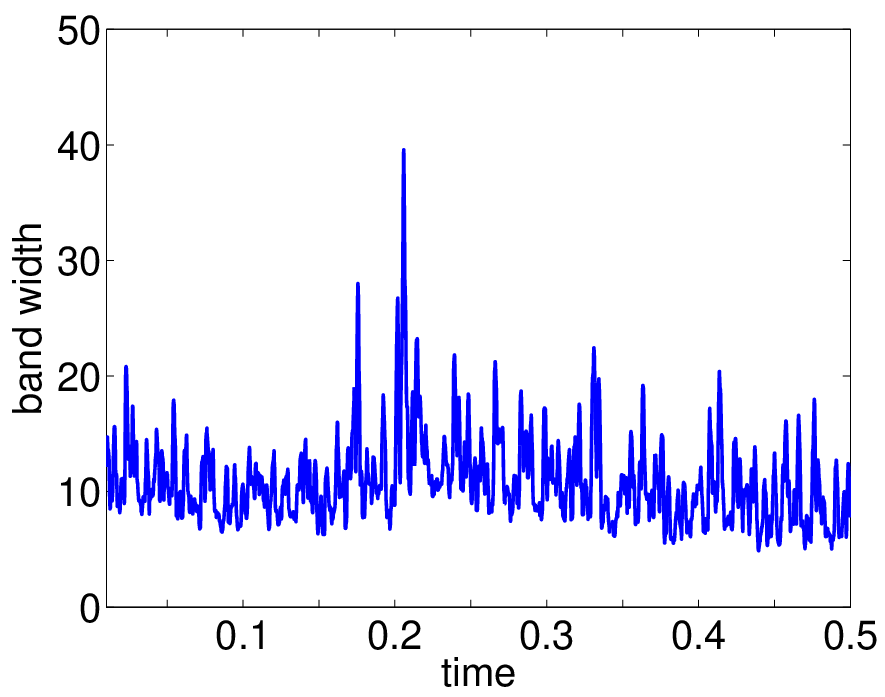
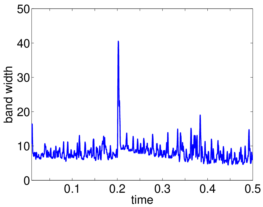
The mean asset value and the corresponding Bollinger bands for a discontinuous background value W⁡(t)W(t) is displayed in Figure 6 (left column). We have chosen d⁡(w)=w⁡(1−w)d(w)=w(1-w) and η=±0.06\eta=\pm 0.06 (upper row) or η=±0.18\eta=\pm 0.18 (lower row). The value W⁡(t)W(t) abruptly decreases at time t=0.2t=0.2. We are interested in the difference of the upper and lower Bollinger bands, more precisely in the Bollinger bandwidth B⁡(t)=100​(R+​(t)−R−​(t))/W⁡(t)B(t)=100(R^{+}(t)-R^{-}(t))/W(t), measuring the relative difference between the upper and lower Bollinger bands. According to chart analysts, falling (increasing) bandwidths reflect decreasing (increasing) volatility. In our simulation, the jump of W⁡(t)W(t) gives rise to a peak of the Bollinger bandwidth at t=0.2t=0.2; see Figure 6 (right column). Another small peak can be observed at t≈0.38t\approx 0.38 (upper right figure) when η=±0.06\eta=\pm 0.06. For larger values of η\eta (lower right figure), the fluctuations in the Bollinger bandwidth are larger.

In chart analysis, the bandwidth is employed to identify a band squeeze. When the asset value leaves the interval [R−,R+][R^{-},R^{+}], this situation may indicate a change of direction of the prices. Clearly, this interpretation cannot be directly applied to the present situation. On the other hand, the Bollinger bands are an additional tool to identify large changes in the mean asset value, for instance when the background value W⁡(t)W(t) is no longer deterministic but driven by some stochastic process. We leave this generalization for future work.

Refer to caption
Refer to caption
Refer to caption
Refer to caption
Figure 6. Mean asset value mw​(f​(t))m_{w}(f(t)) (left column) and Bollinger bands R±​(t)R^{\pm}(t) (right column) versus time. The function W⁡(t)W(t) has a jump at t=0.2t=0.2. The parameters are α=0.05\alpha=0.05, β=0.25\beta=0.25, R=0.025R=0.025, δ=κ=1\delta=\kappa=1. Upper row: η=±0.06\eta=\pm 0.06, lower row: η=±0.18\eta=\pm 0.18.

References

  • [1] E. Altshuler, O. Ramos, Y. Núñez, J. Fernández, A. Batista-Leyva, and C. Noda. Symmetry breaking in escaping ants. Aner. Natur. 166 (2005), 643-649.
  • [2] A. Amadori and R. Natalini. Entropy solutions to a strongly degenerate anisotropic convection-diffusion equation with application to utility theory. J. Math. Anal. Appl. 284 (2003), 511-531.
  • [3] C. Avery and P. Zemsky. Multidimensional uncertainty and herd behavior in financial markets. Amer. Econ. Rev. 88 (1998), 724-748.
  • [4] A. Banerjee. A simple model of herd behavior. Quart. J. Econ. 107 (1992), 797-817.
  • [5] S. Bickhchandani, D. Hirshleifter, and I. Welch. A theory of fads, fashion, custim, and cultural change as informational cascades. J. Polit. Econ. 100 (1992), 992-1026.
  • [6] G. Bird. Molecular Gas Dynamics and the Direct Simulation of Gas Flows. Oxford University Press, Oxford, 1994.
  • [7] L. Boudin and F. Salvarani. A kinetic approach to the study of opinion formation. ESAIM Math. Mod. Anal. Num. 43 (2009), 507-522.
  • [8] M. Brunnermeier. Asset Pricing under Asymmetric Information: Bubbles, Crashes, Technical Analysis, and Herding. Oxford University Press, Oxford, 2001.
  • [9] M. Burger, P. Markowich, and J.-F. Pietschmann. Continuous limit of a crowd motion and herding model: analysis and numerical simulations. Kinetic Related Models 4 (2011), 1025-1047.
  • [10] V. Comincioli, L. Della Croce, and G. Toscani. A Boltzmann-like equation for choice formation. Kinet. Relat. Models 2 (2009), 135-149.
  • [11] S. Cordier, L. Pareschi, and G. Toscani. On a kinetic model for a simple market economy. J. Stat. Phys. 120 (2005), 253-277.
  • [12] P. Degond, C. Appert-Rolland, M. Moussaïd, J. Pettré, and G. Theraulaz. A hierarchy of heuristic-based models of crowd dynamics. J. Stat. Phys. 152 (2013), 1033-1068.
  • [13] M. Delitala and T. Lorenzi. A mathematical model for value estimation with public information and herding. Kinet. Relat. Models 7 (2014), 29-44.
  • [14] A. Devenow and I. Welch. Rational herding in financial economics. Europ. Econ. Rev. 40 (1996), 603-615.
  • [15] B. Düring, P. Markowich, J.-F. Pietschmann, and M.-T. Wolfram. Boltzmann and Fokker-Planck equations modelling opinion formation in the presence of strong leaders. Proc. Roy. Soc. Lond. Ser. A Math. Phys. Eng. Sci. 465 (2009), 3687-3708.
  • [16] B. Düring and M.-T. Wolfram. Opinion dynamics: inhomogeneous Boltzmann-type equations modelling opinion leadership and political segregation. Proc. Roy. Soc. Lond. Ser. A Math. Phys. Eng. Sci. 471 (2015), 20150345.
  • [17] J. Dyer, A. Johansson, D. Helbing, I. Couzin, and J. Krause. Leadership, consensus decision making and collective behaviour in humans. Phil. Trans. Roy. Soc. B: Biol. Sci. 364 (2009), 781-789.
  • [18] M. Escobedo, J.-L. Vázquez, and E. Zuazua. Entropy solutions for diffusion-convection equations with partial diffusivity. Trans. Amer. Math. Soc. 343 (1994), 829-842.
  • [19] W. Hamilton. Geometry for the selfish herd. J. Theor. Biol. 31 (1971), 295-311.
  • [20] T. Hillen, K. Painter, and M. Winkler. Anisotropic diffusion in oriented environments can lead to singularity formation. Europ. J. Appl. Math. 24 (2013), 371-413.
  • [21] D. Hirshleifer. Investor psychology and asset pricing. J. Finance 56 (2001), 1533-1597.
  • [22] L. Pareschi and G. Toscani. Interacting Multiagent Systems. Kinetic Equations and Monte Carlo Methods. Oxford University Press, Oxford, 2014.
  • [23] R. Raafat, N. Chater, and C. Frith. Herding in humans. Trends Cognitive Sci. 13 (2009), 420-428.
  • [24] L. Rook. An economic psychological approach to herd behavior. J. Econ. 40 (2006), 75-95.
  • [25] R. Shiller. Irrational Exuberance. Princeton University Press, Princeton, 2015.
  • [26] G. Toscani. Kinetic models of opinion formation. Commun. Math. Sci. 4 (2006), 481-496.
  • [27] E. Zeidler. Nonlinear Functional Analysis and Applications. Vol. IIA. Springer, New York, 1990.