On the computational complexity of algebraic numbers : the Hartmanis–Stearns problem revisited

This project has received funding from the European Research Council (ERC) under the European Union’s Horizon 2020 research and innovation programme under the Grant Agreement No 648132.

Boris Adamczewski Address: CNRS, Université de Lyon, Université Lyon 1
Institut Camille Jordan
43 boulevard du 11 novembre 1918
69622 Villeurbanne Cedex, France Email: Boris.Adamczewski@math.cnrs.fr Julien Cassaigne Address: CNRS, Aix-Marseille Université
Institut de Mathématiques de Marseille
case 907, 163 avenue de luminy
13288 Marseille Cedex 9, France Email: Julien.Cassaigne@math.cnrs.fr Marion Le Gonidec Address: Université de la Réunion
Laboratoire d’Informatique et de Mathématiques
Parc technologique universitaire, 2 rue Joseph Wetzell
97490 Sainte-Clotilde, France Email: marion.le-gonidec@univ-reunion.fr

Résumé

We consider the complexity of integer base expansions of algebraic irrational numbers from a computational point of view. A major contribution in this area is that the base- $b$ expansion of algebraic irrational real numbers cannot be generated by finite automata. Our aim is to provide two natural generalizations of this theorem. Our main result is that the base- $b$ expansion of algebraic irrational real numbers cannot be generated by deterministic pushdown automata. Incidentally, this completely solves the Hartmanis–Stearns problem for the class of multistack machines. We also confirm an old claim of Cobham from 1968 proving that such real numbers cannot be generated by tag machines with dilation factor larger than one. In order to stick with the modern terminology, we also show that the latter generate the same class of real numbers than morphisms with exponential growth.

1 Introduction

An old source of frustration for mathematicians arises from the study of integer base expansions of classical constants like

\begin{array}[]{cccc}&\sqrt{2}&=&1.414\,213\,562\,373\,095\,048\,801\,688\,724\,209\,698\,078\,569\cdots\\ \text{ or}&&&\\ &\pi&=&3.141\,592\,653\,589\,793\,238\,462\,643\,383\,279\,502\,884\,197\cdots\end{array}

While these numbers admit very simple geometric descriptions, a close look at their digital expansion suggest highly complex phenomena. Over the years, different ways have been envisaged to formalize this old problem. This reoccurring theme appeared in particular in three fundamental papers using : the language of probability after É. Borel [17], the language of dynamical systems after Morse and Hedlund [35], and the language of Turing machines after Hartmanis and Stearns [29]. Each of these points of view leads to a different assortment of challenging conjectures. As its title suggests, the present paper will focus on the latter approach. It is addressed to researchers interested both in Number Theory and Theoretical Computer Science. In this respect, we took care to make the paper as self-contained as possible and hopefully readable by members from these different communities.

After the seminal work of Turing [43], real numbers can be rudely divided into two classes. On one side we find computable real numbers, those whose base- $b$ expansion can be produced by a Turing machine, while on the other side lie uncomputable real numbers which will belong for ever beyond the ability of computers. Note that, though most real numbers belong to the second class, classical mathematical constants are usually computable. This is in particular the case of any algebraic number. However, among computable numbers, some are quite easy to compute while others seem to have an inherent complexity that make them difficult to compute. In 1965, Hartmanis and Stearns [29] investigated the fundamental question of how hard a real number may be to compute, introducing the now classical time complexity classes. The notion of time complexity takes into account the number $T(n)$ of operations needed by a multitape deterministic Turing machine to produce the first $n$ digits of the expansion. In this regard, a real number is considered all the more simple as its base- $b$ expansion can be produced very fast by a Turing machine. At the end of their paper, Hartmanis and Stearns suggested the following problem.

Problem HS. — Do there exist irrational algebraic numbers for which the first $n$ binary digits can be computed in $O(n)$ operation by a multitape deterministic Turing machine ?

Let us briefly recall why Problem HS is still open and likely uneasy to solve. On the one hand, all known approaches to compute efficiently the base- $b$ expansion of algebraic irrational numbers intimately relate on the cost of the multiplication $M(n)$ of two $n$ -digits numbers (see for instance [18]). This operation is computable in quasilinear time¹¹ 1 This means computable in $O(n\log^{1+\varepsilon}n)$ operations for some $\varepsilon$ . but to determine whether one may have $M(n)=O(n)$ or not remains a famous open problem in this area. On the other hand, a negative answer to Problem HS²² 2 As observed in [26], this may be the less surprising issue. would contain a powerful transcendental statement, a very special instance of which is the transcendence of the following three simple irrational real-time computable numbers :

\sum_{n=1}^{\infty}\frac{1}{2^{n!}}\;,\;\sum_{n=1}^{\infty}\frac{1}{2^{n^{2}}}\;\mbox{ and }\sum_{n=1}^{\infty}\frac{1}{2^{n^{3}}}\,\cdot

Of course, for the first one, Liouville’s inequality easily does the job. But the transcendance of the second number only dates back to 1996 [16, 28] and its proof requires the deep work of Nesterenko about algebraic independence of values of Eisenstein’s series [37]. Finally, the transcendence of the third number remains unknown.

In 1968, Cobham [26] (see also [24, 25]) was the first to consider the restriction of the Hartmanis-Stearns problem to some classes of Turing machines. The model of computation he originally investigated is the so-called Tag machine. Though this model has some historical interest, this terminology is not much used today by the computer science community. However, their outputs precisely correspond to the class of morphic sequences, a well-known object of interest for both mathematicians and computer scientists. They are especially used in combinatorics on words and symbolic dynamics (see for instance [12, 40, 41]). In the sequel, we will present our result with this modern terminology but, for the interested reader, we will still describe the connection with tag machines in Section 5.1. In his paper, Cobham stated two main theorems without proof and only gave some hints that these statements should be deduced from a general transcendence method based on some functional equations, now known as Mahler’s method. His first claim was finally confirmed by the first author and Bugeaud [3], but using a totally different approach based on a $p$ -adic version of the subspace Theorem (see [3, 8])³³ 3 Very recently, some advances in Mahler’s method [39, 10] allow to complete the proof originally envisaged by Cobham..

Theorem AB (Cobham’s first claim). — The base- $b$ expansion of an algebraic irrational number cannot be generated by a uniform morphism or, equivalently, by a finite automaton.

Remark 1.1.

Theorem AB actually refers to two conceptually quite different models of computation : uniform morphisms and finite automata. There are two natural ways a multitape deterministic Turing machine can be used to define computable numbers. First, it can be considered as enumerator, which means that the machine will produce one by one all the digits, separated by a special symbol, on its output tape. Problem HS originally referred to the model of enumerators. The other way, referred to as Turing transducer, consists in feeding to the machine some input representing a positive integer $n$ and asking that the machine compute the $n$ -th digit on its output tape. In Theorem AB, uniform morphisms (or originally uniform tag machines) are enumerators while finite automata are used as transducers⁴⁴ 4 Note that, used as enumerators, finite automata can only produce eventually periodic sequences of digits and thus rational numbers. In contrast, used as transducers, finite automata output the interesting class of automatic sequences.. The fact that these two models are equivalent is due to Cobham [27].

Theorem AB is the main contribution up to date toward a negative solution to Problem HS. In this paper, we show that the approach developed in [3, 8] leads to two interesting generalizations of this result. Our first generalization is concerned with enumerators. In this direction, we confirm the second claim of Cobham.

Theorem 1.2 (Cobham’s second claim).

The base- $b$ expansion of an algebraic irrational number cannot be generated by a morphism with exponential growth.

We stress that, stated as this, Theorem 1.2 also appeared in the Thèse de Doctorat of Julien Albert [11]. In order to provide a self-contained proof of Cobham’s second claim, which was originally formulated in terms of tag machines, we will complete and reprove with permission some content of [11] in Section 4.1. The fact that Theorem 1.2 is well equivalent to Cobham’s second claim will be proved in Section 5.1.

Our second and main generalization of Theorem AB is concerned with transducers. We consider a classical computation model called the deterministic pushdown automaton. It is of great importance on the one hand for theoretical aspects because of Chomsky’s hierarchy [23] in formal language theory and on the other for practical applications, especially in parsing (see [30]). Roughly, such a device is a finite automaton with in addition a possibly infinite memory organized as a stack. Our main result is the following.

Theorem 1.3.

The base- $b$ expansion of an algebraic irrational number cannot be generated by a deterministic pushdown automaton.

In Section 5.2, we use Theorem 1.3 to revisit the Hartmanis–Stearns problem as follows : instead of some time constraint, we put some restriction based on the way the memory may be stored by Turing machines. This leads us to consider a classical computation model called multistack machine. It corresponds to a version of the deterministic Turing machine where the memory is simply organized by stacks. It is as general as the Turing machine if one allows two or more stacks. Furthermore the one-stack machine turns out to be equivalent to the deterministic pushdown automaton, while a zero-stack machine is just the finite automaton of Theorem AB, that is a machine with a strictly finite memory only stored in the finite state control. Incidentally, Theorems AB and 1.3 turn out to completely solve the Hartmanis–Stearns problem for multistack machines. Our approach also provides a method to prove the transcendence of some real numbers generated by linearly bounded Turing machines (see the example in Section 5.3).

This paper is organized as follows. Definitions related to finite automata, morphisms, and pushdown automata are given in Section 2. The useful combinatorial transcendence criterion of [8], on which our results are based, is recalled in Section 3. Section 4 is devoted to the proofs of our main results : Theorems 1.2 and 1.3. In connection with these results, two models of computation are discussed in Section 5 : the tag machine and the multistack machine. Finally, Section 6 is devoted to concluding remarks regarding factor complexity, some quantitative aspects of this method, and continued fractions.

2 Finite automata, morphic sequences and pushdown automata

In this section, we give definitions for a real number to be generated by a finite automaton, a morphism, and a deterministic pushdown automaton. This provides a precise meaning to Theorems AB, 1.2, and 1.3.

All along this paper, we will use the following notations. An alphabet $A$ is a finite set of symbols, also called letters. A finite word over $A$ is a finite sequence of letters in $A$ or equivalently an element of $A^{*}$ , the free monoid generated by $A$ . The length of a finite word $W$ , that is the number of symbols composing $W$ , is denoted by $|W|$ . We will denote by $\epsilon$ the empty word, that is the unique word of length $0$ , and $A^{+}$ the set of finite words of positive length over $A$ . If $a$ is a letter and $W$ a finite word, then $|W|_{a}$ stands for the number of occurrences of the letter $a$ in $W$ . Let $k\geq 2$ be a natural number. We let $\Sigma_{k}$ denote the alphabet $\left\{0,1,\ldots,k-1\right\}$ . Given a positive integer $n$ , we set $\langle n\rangle_{k}:=w_{r}w_{r-1}\cdots w_{1}w_{0}$ for the base- $k$ expansion of $n$ , which means that $n=\sum_{i=0}^{r}w_{i}k^{i}$ with $w_{i}\in\Sigma_{k}$ and $w_{r}\not=0$ . Note that by convention $\langle 0\rangle_{k}:=\epsilon$ . Conversely, if $w:=w_{1}\cdots w_{r}$ is a finite word over the alphabet $\Sigma_{k}$ , we set $[w]_{k}:=\sum_{i=0}^{r}w_{r-i}k^{i}$ . The usual notations $\{x\}$ , $\lfloor x\rfloor$ , and $\lceil x\rceil$ respectively stand for the fractional part, the floor, and the ceil of the real number $x$ .

2.1 Finite automata and automatic sequences

A sequence ${\bf a}:=(a_{n})_{n\geq 0}$ with values in a finite set is $k$ -automatic if it can be generated by a finite automaton used as a transducer. This means that there exists a finite-state machine (a deterministic finite automaton with output) that takes as input the base- $k$ expansion of $n$ and produces as output the symbol $a_{n}$ .

Let us give now a formal definition of a $k$ -automatic sequence. Let $k\geq 2$ be a natural number. A $k$ -automaton is defined as a $6$ -tuple $\displaystyle{\mathcal{A}}=\left(Q,\Sigma_{k},\delta,q_{0},\Delta,\tau\right),$ where :

—

$Q$ is a finite set of states,
—

$\delta:Q\times\Sigma_{k}\rightarrow Q$ is the transition function,
—

$q_{0}$ is the initial state,
—

$\Delta$ is the output alphabet,
—

and $\tau:Q\rightarrow\Delta$ is the output function.

Given a state $q$ in $Q$ and a finite word $w=w_{1}w_{2}\cdots w_{n}$ on the alphabet $\Sigma_{k}$ , we define $\delta(q,w)$ recursively by $\delta(q,w)=\delta(\delta(q,w_{1}w_{2}\cdots w_{n-1}),w_{n})$ .

Definition 2.1.

Let $\displaystyle{\mathcal{A}}=\left(Q,\Sigma_{k},\delta,q_{0},\Delta,\tau\right)$ be a $k$ -automaton. The output sequence produced by $\mathcal{A}$ is the sequence $(\tau(\delta(q_{0},\langle n\rangle_{k})))_{n\geq 1}$ . Such a sequence is called a $k$ -automatic sequence. A sequence or an infinite word is said to be automatic if it is $k$ -automatic for some integer $k\geq 2$ .

Example 2.2.

By a classical result of Lagrange, it is known that every non-negative integer can be written as the sum of four perfect squares. It is optimal in the sense that some natural numbers cannot be written as the sum of only three square numbers. More precisely, Legendre proved that

\exists\,a,b,c\mid n=a^{2}+b^{2}+c^{2}\iff\not\exists\,i,j\mid n=4^{i}(8j+7)\,,

where $n,a,b,c,i,j$ are nonnegative integers. As a consequence, the binary sequence ${\bf s}:=(s_{n})_{n\geq 0}$ defined by $s_{n}=1$ if $n$ can be written as the sum of three squares and $s_{n}=0$ otherwise is $2$ -automatic.

0,2)(6,-3) nclineawa nccurveaanaput[npos=.25] $0$ nccurveddnbput[npos=.25] $1$ ncarcabnbput[npos=.40] $1$ ncarcbanbput[npos=.40] $0$ ncarcebnbput[npos=.40] $1$ ncarcefnbput[npos=.40] $0$ ncarcfenbput[npos=.40] $0$ ncarcfbnaput[npos=.40] $1$ ncarccanbput[npos=.40] $0$ ncarccdnaput[npos=.40] $1$ ncarcbcnbput[npos=.40] $1$ ncarcdenbput[npos=.40] $0$

Figure 2.1: A

2

-automaton generating the sequence

{\bf s}

Definition 2.3.

A real number $\xi$ can be generated by a deterministic $k$ -automaton $\mathcal{A}$ if, for some integer $b\geq 2$ , one has $\langle\{\xi\}\rangle_{b}=0.a_{1}a_{2}\cdots$ , where $(a_{n})_{n\geq 1}$ corresponds to the output sequence produced by $\mathcal{A}$ .

Theorem AB thus implies that the binary number

\xi_{0}:=1.111\,111\,011\,111\,110\,111\,111\,111\,111\,011\,011\,111\,110\cdots

generated by the $2$ -automaton of Figure 2.1 is transcendental.

2.2 Morphic sequences

As already mentioned in the introduction, Cobham suggested in 1968 to restrict Problem HS to a special class of real-time Turing machines called tag machines. Though these machines have an historical interest, this terminology is not much used today by the computer science community. However, their outputs precisely correspond to class of morphic sequences that we define below. In contrast, the latter are well-known objects of interest for both mathematicians and computer scientists. For the interested reader, we will still describe tag machines in Section 5.1.

We recall here some basic definitions. Let $A$ be a finite alphabet. A map from $A$ to $A^{*}$ naturally extends to a map from $A^{*}$ into itself called (endo)morphism. Given two alphabets $A$ and $B$ , a map from $A$ to $B$ naturally extends to a map from $A^{*}$ into $B^{*}$ called a coding or letter-to-letter morphism. A morphism $\sigma$ over $A$ is said to be $k$ -uniform if $|\sigma(a)|=k$ for every letter $a$ in $A$ , and just uniform if it is $k$ -uniform for some $k$ . A useful object associated with a morphism $\sigma$ is the so-called incidence matrix of $\sigma$ , denoted by $M_{\sigma}$ . We first need to choose an ordering of the elements of $A$ , say $A=\{a_{1},a_{2},\ldots,a_{d}\}$ , and then $M_{\sigma}$ is defined by

\forall i,j\in\{1,\ldots,d\},\;\;\left(M_{\sigma}\right)_{i,j}:=|\sigma(a_{j})|_{a_{i}}\,.

The choice of the ordering has no importance. A morphism $\sigma$ over $A$ is said to be prolongable on $a$ if $\sigma(a)=aW$ for some word $W$ and if the length of the word $\sigma^{n}(a)$ tends to infinity with $n$ . Then the word

\sigma^{\omega}(a):=\lim_{n\to\infty}\sigma^{n}(a)=aW\sigma(W)\sigma^{2}(W)\cdots

is the unique fixed point of $\sigma$ that begins with $a$ . An infinite word obtained by iterating a prolongeable morphism $\sigma$ is said to be purely morphic. The image of a purely morphic word under a coding is a morphic word. Thus to define a morphic word ${\bf a}$ one needs a $5$ -tuple ${\mathcal{T}}=(A,\sigma,a,B,\varphi)$ such that ${\bf a}=\varphi(\sigma^{\omega}(a))$ , where :

—

$A$ is a finite set of symbols called the internal alphabet.
—

$a$ is a an element of $A$ called the starting symbol.
—

$\sigma$ is a morphism of $A^{*}$ prolongable on $a$ .
—

$B$ is a finite set of symbols called the external alphabet.
—

$\varphi$ is a letter-to-letter morphism from $A$ to $B$ .

When $\sigma$ is uniform (resp. $k$ -uniform, ), the sequence ${\bf a}$ is said to be generated by a uniform (resp. $k$ -uniform) morphism.

Definition 2.4.

A morphism $\sigma$ is said to have exponential growth if the spectral radius of the matrix $M_{\sigma}$ is larger than one. When $\sigma$ has exponential growth and all letters of $A$ appear in $\sigma^{\omega}(a)$ , the sequence ${\bf a}=\varphi(\sigma^{\omega}(a))$ is said to be generated by a morphism with exponential growth.

Definition 2.5.

A real number $\xi$ can be generated by a morphism with exponential growth if, for some integer $b\geq 2$ , one has $\langle\{\xi\}\rangle_{b}=0.a_{1}a_{2}\cdots$ , where ${\bf a}:=(a_{n})_{n\geq 1}$ can be generated by a morphism with exponential growth.

Theorem 1.2 thus implies the transcendence of the ternary number

\xi_{1}:=0.021\,201\,220\,210\,122\,202\,120\,120\,210\,122\,220\,212\,122\cdots

whose expansion is the sequence ${\bf a}=\varphi_{1}(\sigma_{1}^{\omega}(a))$ , where $\sigma_{1}(a)=acb$ , $\sigma_{1}(b)=abc$ , $\sigma_{1}(c)=c$ , $\varphi_{1}(a)=0$ , $\varphi_{1}(b)=1$ , and $\varphi_{1}(c)=2$ . One can check that $\sigma_{1}$ has exponential growth for the spectral radius of $M_{\sigma_{1}}=2$ . In contrast, Theorem 1.2 does not apply to prove the transcendence of binary number $\displaystyle\sum_{n=1}^{\infty}\frac{1}{2^{n^{2}}}$ . Indeed, though this number can be generated by a morphism, the latter has non-exponential growth. Indeed the characteristic sequence of squares can be obtained as $\varphi_{2}(\sigma_{2}^{\omega}(a))$ where $\sigma_{2}(a)=ab$ , $\sigma_{2}(b)=ccb$ , $\sigma_{2}(c)=c$ , $\varphi_{2}(a)=\varphi_{2}(c)=0$ , and $\varphi_{2}(b)=1$ . One can check easily that the spectral radius of $M_{\sigma_{2}}=1$ .

Remark 2.6.

Following Cobham [26], there is no loss of generality to assume than the internal morphism $\sigma$ is a non-erasing morphism, which means that no letter is mapped to the empty word. Indeed, if an infinite word can be generated by an erasing morphism , then there also exists a non-erasing morphism that can generate it. From now on, we will thus only consider non-erasing morphisms.

It is worth mentioning that the class of sequences generated by uniform morphisms is especially relevant because of the following result of Cobham [27].

Proposition C. — A sequence is $k$ -automatic if and only if it can be generated by some $k$ -uniform morphism.

Furthermore the proof of Proposition C is completely constructive and provides a simple way to go from $k$ -uniform morphisms to $k$ -automata and vice versa. This general feature is examplified below. For a complete treatment see [27] or Chapter 6 of [12].

Example 2.7.

The Thue--Morse sequence ${\bf t}:=(t_{n})_{n\geq 0}$ is probably the most famous example among automatic sequences. It is defined as follows : $t_{n}=0$ if the sum of the binary digits of $n$ is even, and $t_{n}=1$ otherwise. It can be generated by the following finite $2$ -automaton : ${\mathcal{A}}=\left(\{q_{0},q_{1}\},\{0,1\},\delta,q_{0},\{0,1\},\tau\right)$ , where $\delta(q_{0},0)=\delta(q_{1},1)=q_{0}$ , $\delta(q_{0},1)=\delta(q_{1},0)=q_{1}$ , $\tau(q_{0})=0$ and $\tau(q_{1})=1$ .

0,-1)(4,2) nclineawa nccurveaanaput[npos=.25] $0$ nccurvebbnaput[npos=.25] $0$ ncarcabnaput[npos=.40] $1$ ncarcbanaput[npos=.40] $1$

Figure 2.2: A

2

-automaton generating Thue–Morse sequence.

The Thue–Morse sequence can be as well generated by a $2$ -uniform morphism for one has ${\bf t}=\varphi(\sigma^{\omega}(q_{0}))$ , where $\sigma(q_{0})=q_{0}q_{1}$ , $\sigma(q_{1})=q_{1}q_{0}$ , $\varphi(q_{0})=0$ , $\varphi(q_{1})=1$ .

2.3 Pushdown automata

A pushdown automaton is a classical device, but most often used in formal language theory as an acceptor, that is a machine that can accept or reject finite words and langages, namely context-free languages (see for instance [13, 14, 30]). Our point of view here is slightly different for we will use the pushdown automaton as a transducer, that is a machine that associates a symbol with every finite word on a given input alphabet.

Formally, a $k$ -pushdown automaton is a complete deterministic pushdown automaton with output, or DPAO for short. It is defined as a 7-tuple $\mathcal{M}=(Q,\Sigma_{k},\Gamma,\delta,q_{0},\Delta,\tau)$ where :

—

$Q$ is a finite set of states,
—

$\Sigma_{k}:=\{0,1,\ldots,k-1\}$ is the finite set of input symbols,
—

$\Gamma$ is the finite set of stack symbols. A special symbol $\#$ is used to mark the bottom of the stack.
For convenience, we identify $\#$ with the empty word of $\Gamma^{*}$ .
—

$\delta:E\subset Q\times\left(\Gamma\cup\{\#\}\right)\times\left(\Sigma_{k}\cup\{\varepsilon\}\right)\to Q\times\Gamma^{*}$ is the transition function,
—

$q_{0}\in Q$ is the initial state and $(q_{0},\#)$ is the initial (internal) configuration,
—

$\Delta$ is the finite set of output symbols,
—

$\tau:Q\times\Gamma\cup\{\#\}\to\Delta$ is the output function.

Furthermore, the transition function satisfies the following conditions.

—

Determinism assumption : if $(q,a,\epsilon)$ belongs to $E$ for some $(q,a)\in Q\times\left(\Gamma\cup\{\#\}\right)$ , then for every $i\in\Sigma_{k}$ , $(q,a,i)\not\in E$ .
—

Completeness assumption : If $(q,a,\epsilon)$ does not belong to $E$ for some $(q,a)\in Q\times\left(\Gamma\cup\{\#\}\right)$ , then $\{q\}\times\{a\}\times\Sigma_{k}\subset E$ .

Remark 2.8.

Notice that $\delta$ being a function is also a part of the determinism assumption. In a nondeterministic $k$ -pushdown automata, $\delta$ would be only define as a subset of $Q\times\left(\Gamma\cup\{\#\}\right)\times\left(\Sigma_{k}\cup\{\epsilon\}\right)\times Q\times\Gamma^{*}$ .

We want now to make sense to the computation $\tau(\delta(q_{0},\#,W))$ for any input word $W$ in $\Sigma_{k}^{*}$ . First the transition function $\delta$ of a $k$ -pushdown automaton can naturally be extended to a subset of $Q\times\Gamma^{*}\times\left(\Sigma_{k}\cup\{\epsilon\}\right)$ by setting

\forall S=s_{1}\cdots s_{j}\in\Gamma^{*},|S|\geq 2\,,\;\;\delta(q,S,a)=(q^{\prime},s_{1}\cdots s_{j-1}X)\,,

when $\delta(q,s_{j},a)=(q^{\prime},X)$ . After reading the symbol $a$ , the pushdown automaton could have reached a configuration $(q,S)$ from which $\epsilon$ -moves are possible. In such a case, one asks the pushdown automaton to perform all possible $\epsilon$ -moves before reading the next input symbol. We stress that this appears to be a classical convention (see the discussion in [14]) which can be formalized as follows. We define the function $\overline{\delta}$ by :

\overline{\delta}(q,S,a)=\left\{\begin{array}[]{cl}\delta(q,S,a)&\mbox{if }(\delta(q,S,a),\epsilon)\notin E\\ \overline{\delta}(\delta(q,S,a),\epsilon)&\mbox{if }(\delta(q,S,a),\epsilon)\in E\end{array}\right.

Then $\overline{\delta}$ can be extended to a subset of $Q\times\Gamma^{*}\times\Sigma_{k}^{*}$ by setting

\overline{\delta}(q,S,w_{1}\cdots w_{r})=\overline{\delta}\left(\overline{\delta}\left(q,S,w_{1}\cdots w_{r-1}\right),w_{r}\right)\,.

This means in particular that $\mathcal{M}$ scans its inputs from left to right. From now on, we will not distinguish $\delta$ from its extension $\overline{\delta}$ . We also extend the output function $\tau$ to a subset of $Q\times\Gamma^{*}$ by simply setting $\tau(q,s_{1}s_{2}\cdots s_{j})=\tau(q,s_{j})$ .

Definition 2.9.

Let $\mathcal{M}=(Q,\Sigma_{k},\Gamma,\delta,q_{0},\Delta,\tau)$ be a $k$ -pushdown automaton. The sequence $(\tau(\delta(q_{0},\#,\langle n\rangle_{k})))_{n\geq 1}$ is called the output sequence produced by $\mathcal{M}$ .

This class of sequences are discussed in [22]. They form a subclass of context-free sequences (see [32, 36]).

Example 2.10.

Usually a deterministic pushdown automaton is represented as a finite graph whose vertices are labelled by the elements of $Q$ and whose edges are labelled by transitions as follows : $\delta(q,S,a)=q^{\prime}W$ is represented by the edge $q\xrightarrow{(a,S|W)}q^{\prime}$ . An example of such internal representation is given by the $2$ -pushdown automaton $\mathcal{A}$ in Figure 2.3. It outputs the binary sequence

{\bf a}:=1110111001101000011111101110100000010110\cdots

whose $n$ -th binary digit is $1$ if the difference between the number of occurrences of the digits $0$ and $1$ in the binary expansion of $n$ is at most $1$ , and is $0$ otherwise.

-5,-1)(5,1.5) nclineqnq nccurveppnaput[npos=.5] $\begin{array}[]{l}(1,\#|X),\\ (1,X|XX),\\ (0,X|\#)\end{array}$ ncarcpqnaput[npos=.5] $(0,\#|\#)$ ncarcqpnaput[npos=.5] $(1,\#|\#)$ ncarcrqnaput[npos=.5] $(1,\#|\#)$ ncarcqrnaput[npos=.5] $(0,\#|\#)$ nccurverrnbput[npos=.5] $\begin{array}[]{l}(0,\#|X),\\ (0,X|XX),\\ (1,X|\#)\end{array}$

Figure 2.3: A

2

-pushdown automaton producing the binary expansion of

\xi_{2}

This automaton works as follows. Being on state $q_{0}$ means that the part of the input word that has been already read contains as many $1$ ’s as $0$ ’s. On the other hand, being on state $q_{1}$ means that the part of the input word that has been already read contains more $1$ ’s than $0$ ’s, while being on state $q_{-1}$ means that it contains more $0$ ’s than $1$ ’s. Furthermore, in any of these two states, the difference between the number of $0$ ’s and $1$ ’s (in absolute value) is one more than the number of $X$ ’s in the stack. Thus, the difference between the number of occurrences of the symbols $1$ and $0$ in the input word is at most $1$ if, and only if, the reading ends with an empty stack (regardless to the ending state). By definition of the output function, we see that $\mathcal{A}$ well produces the infinite word ${\bf a}$ .

Note that, formally, this pushdown automaton should be defined as : $\mathcal{A}:=(\{q_{0},q_{1},q_{-1}\},\Sigma_{2},\{X\},\delta,q_{0},\{0,1\},\tau)$ , where the transition function $\delta$ is defined by $\delta(q_{0},\#,1)=(q_{1},\#)$ , $\delta(q_{0},\#,0)=(q_{-1},\#)$ , $\delta(q_{1},\#,0)=(q_{0},\#)$ , $\delta(q_{1},\#,1)=(q_{1},X)$ , $\delta(q_{1},X,0)=(q_{1},\#)$ , $\delta(q_{1},X,1)=(q_{1},XX)$ , $\delta(q_{-1},\#,0)=(q_{-1},X)$ , $\delta(q_{-1},\#,1)=(q_{0},\#)$ , $\delta(q_{-1},X,0)=(q_{-1},XX)$ , $\delta(q_{-1},X,1)=(q_{-1},\#)$ , and where the output function $\tau$ is defined by $\tau(q_{0},\#)=\tau(q_{1},\#)=\tau(q_{-1},\#)=1$ , and $\tau(q_{0},X)=\tau(q_{1},X)=\tau(q_{-1},X)=0$ .

Definition 2.11.

A real number $\xi$ can be generated by a deterministic $k$ -pushdown automaton $\mathcal{M}$ if, for some integer $b\geq 2$ , one has $\langle\{\xi\}\rangle_{b}=0.a_{1}a_{2}\cdots$ , where $(a_{n})_{n\geq 1}$ corresponds to the output sequence produced by $\mathcal{M}$ .

Theorem 1.3 thus implies the transcendence of the binary number

\xi_{2}:=1.110\,111\,001\,101\,000\,011\,111\,101\,110\,100\,000\,010\,110\cdots

whose binary expansion is the infinite word ${\bf a}$ of Example 2.10.

Remark 2.12.

About $\epsilon$ -moves.— Since we only consider deterministic pushdown automata, we can assume without loss of generality that all $\epsilon$ -moves are decreasing (see for instance [14]). This means that a computation of the form $\delta(q,W,\epsilon)=(q^{\prime},W^{\prime})$ , always implies that $|W^{\prime}|<|W|$ .

About input words— In our model of $k$ -pushdown automaton, we choose to feed our machines only with the proper base- $k$ expansion of each nonnegative integer $n$ . Instead, we could as well imagine to ask that $\tau(\delta(q_{0},\#,w))$ remains the same for all words $w\in\Sigma_{k}^{*}$ such that $[w]_{k}=n$ , that is $\tau(\delta(q_{0},\#,w))=\tau(\delta(q_{0},\#,0^{j}w))$ for every natural number $j$ . Such a change would not affect the class of output sequences produced by $k$ -pushdown automata. The discussion is similar to the case of the $k$ -automaton and we refer to [12] for more details.

Our second remark concerning inputs is more important. In our model, the $k$ -pushdown automaton scans the base- $k$ expansion of a positive integer $n$ starting from the most significant digit. This corresponds to the usual way humans read numbers, that is from left to right. In the case of the $k$ -automaton, this choice is of no consequence because both ways of reading are known to be equivalent. However, this is no longer true for $k$ -pushdown machines as the class of deterministic context free languages is not closed under mirror image.

About uniqueness— There always exist several different $k$ -pushdown automata producing the same output. In particular, it is possible to choose one with a single state (see for instance [13]). The $2$ -automaton given in Figure 2.3 is certainly not the smallest one with respect to the number of states, but it makes the process of computation more transparent and it only uses one ordinary stack symbol.

3 A combinatorial transcendence criterion

In this section, we recall the fundamental relation between Diophantine approximation and repetitive patterns occurring in integer base expansions of real numbers.

Let $A$ be an alphabet and $W$ be a finite word over $A$ . For any positive integer $k$ , we write $W^{k}$ for the word

\underbrace{W\cdots W}_{\mbox{$k$ times}}

(the concatenation of the word $W$ repeated $k$ times). More generally, for any positive real number $x$ , $W^{x}$ denotes the word $W^{\lfloor x\rfloor}W^{\prime}$ , where $W^{\prime}$ is the prefix of $W$ of length $\left\lceil\{x\}|W|\right\rceil$ . The following natural measure of periodicity for infinite words was introduced in [4] (see also [1, 9]).

Definition 3.1.

The Diophantine exponent of an infinite word ${\bf a}$ is defined as the supremum of the real numbers $\rho$ for which there exist arbitrarily long prefixes of ${\bf a}$ that can be factorized as $UV^{\alpha}$ , where $U$ and $V$ are two finite words ( $U$ possibly empty) and $\alpha$ is a real number such that

\frac{|UV^{\alpha}|}{|UV|}\geq\rho.

The Diophantine exponent of ${\bf a}$ is denoted by ${{\rm dio}}({\bf a})$ .

Of course, for any infinite word ${\bf a}$ one has the following relation

1\leq{\rm dio}({\bf a})\leq+\infty.

Furthermore, ${\rm dio}({\bf a})=+\infty$ for an eventually periodic word ${\bf a}$ , but the converse is not true. There is some interesting interplay between the Diophantine exponent and Diophantine approximation, which is actually reponsible for the name of the exponent. Let $\xi$ be a real number whose base- $b$ expansion is $0.a_{1}a_{2}\cdots$ . Set ${\bf a}:=a_{1}a_{2}\cdots$ . Let us assume that the word ${\bf a}$ begins with a prefix of the form $UV^{\alpha}$ . Set $q=b^{|U|}(b^{|V|}-1)$ . A simple computation shows that there exists an integer $p$ such that

\langle p/q\rangle_{b}=0.UVVV\cdots.

Since $\xi$ and $p/q$ have the same first $|UV^{\alpha}|$ digits in their base- $b$ expansion, we obtain that

\left|\xi-\frac{p}{q}\right|<\frac{1}{b^{|UV^{\alpha}|}}

and thus

\left|\xi-\frac{p}{q}\right|<\frac{1}{q^{\rho}},

(3.1)

where $\rho=|UV^{\alpha}|/|UV|$ .

We do not claim here that $p/q$ is written in lowest terms. Actually, it may well happen that the $\gcd$ of $p$ and $q$ is quite large but (3.1) still holds in that case. By Definition 3.1, it follows that if ${\rm dio}({\bf a})=\mu$ , then for every $\rho<\mu$ , there exists infinitely many rational numbers $p/q$ such that

\left|\xi-\frac{p}{q}\right|<\frac{1}{q^{\rho}}\cdot

Note that when ${\rm dio}({\bf a})<2$ , such approximations look quite bad, for the existence of much better ones is ensured by the theory of continued fractions or by Dirichlet pigeonhole principle. Quite surprisingly, the inequality ${\rm dio}({\bf a})>1$ is already enough to conclude that $\xi$ is either rational or transcendental. This powerful combinatorial transcendence criterion, proved in [8] and restated in Proposition ABL, emphasizes the relevance of the Diophantine exponent for our purpose.

Proposition ABL. — Let $\xi$ be a real number with $\langle\{\xi\}\rangle_{b}:=0.a_{1}a_{2}\cdots$ . Let us assume that ${\rm dio}({\bf a})>1$ where ${\bf a}:=a_{1}a_{2}\cdots$ . Then $\xi$ is either rational or transcendental.

Proposition ABL is obtained as a consequence of the $p$ -adic Subspace Theorem. It is the key tool for proving Theorem AB and it will be the key tool for proving Theorems 1.2 and 1.3 as well. In this section, we recall the fundamental relation between Diophantine approximation and repetitive patterns occurring in integer base expansions of real numbers.

4 Proof of Theorems 1.2 and 1.3

In this section, we prove our two main results.

4.1 Proof of Theorem 1.2

In order to prove Theorem 1.2, we first need the following definition.

Definition 4.1.

Let $A$ be a finite set and $\sigma$ be a morphism of $A^{*}$ . A letter $b\in A$ is said to have maximal growth if there exists a real number $C$ such that

|\sigma^{n}(c)|<C|\sigma^{n}(b)|\,,

for every letter $c\in A$ and every positive integer $n$ .

Lemma 4.2.

Let $A$ be a finite set and $a\in A$ . Let $\sigma$ be a morphism of $A^{*}$ prolongable on $a$ and such that all letters of $A$ appear in $\sigma^{\omega}(a)$ . Let $\theta$ denote the spectral radius of $M_{\sigma}$ . Then the letter $a$ has maximal growth.

Furthermore, there exist a nonnegative integer $k$ , and two positive real numbers $c_{1}$ and $c_{2}$ such that

c_{1}n^{k}\theta^{n}<|\sigma^{n}(a)|<c_{2}n^{k}\theta^{n}\,.

(4.1)

Démonstration.

Let $c$ be a letter occurring in $\sigma^{\omega}(a)$ . Then $c$ also occurs in $\sigma^{r}(a)$ , for some positive integer $r$ . Then

|\sigma^{n}(c)|\leq|\sigma^{n+r}(a)|=|\sigma^{r}(\sigma^{n}(a))|\leq\|M_{\sigma^{r}}\|_{\infty}|\sigma^{n}(a)|\,,

where $\|\cdot\|_{\infty}$ stands for the usual infinite norm. This shows that $a$ has maximal growth. Recall now that by a classical result of Salomaa and Soittola (see for instance Theorem 4.7.15 in [21]), there exist a nonnegative integer $k$ , a real number $\beta\geq 1$ , and two positive real numbers $c_{1}$ and $c_{2}$ such that

c_{1}n^{k}\beta^{n}<|\sigma^{n}(a)|<c_{2}n^{k}\beta^{n}\,,

(4.2)

for every positive integer $n$ . Since $a$ has maximal growth, a classical theorem on matrices due to Gelfand (see for instance [21]) implies that $\beta$ must be equal to $\theta$ , the spectral radius of the incidence matrix of $\sigma$ . ∎

Proposition 4.3.

Let ${\bf a}$ denote an infinite sequence than can be generated by a morphism with exponential growth. Then ${\rm dio}({\bf a})>1$ .

Démonstration.

Let ${\bf a}$ denote an infinite sequence than can be generated by a morphism with exponential growth. Then ${\bf a}=\varphi(\sigma^{\omega}(a))$ for some morphism $\sigma$ with exponential growth defined over a finite alphabet $A$ , and some coding $\varphi$ . Furthermore, we recall that the spectral radius $\theta$ of the incidence matrix $M_{\sigma}$ satisfies $\theta>1$ . Set ${\bf u}:=\sigma^{\omega}(a)$ . Since by definition $\sigma$ is prolongable on $a$ and all letters of $A$ appear in ${\bf u}$ , Lemma 4.2 implies that $a$ has maximal growth and that there exist two positive real numbers $c_{1}$ and $c_{2}$ such that

c_{1}n^{k}\theta^{n}<|\sigma^{n}(a)|<c_{2}n^{k}\theta^{n},

(4.3)

for every positive integer $n$ .

We now prove that there are infinitely many occurrences of letters with maximal growth in ${\bf u}$ . Let us argue by contradiction. If there are only finitely many occurrences of letters with maximal growth, then there exists a positive integer $n_{0}$ such that ${\bf u}=\sigma^{n_{0}}(a){\bf w}$ where ${\bf w}$ is an infinite word that contains no letter with maximal growth. Since $\theta>1$ , there is an integer $m_{0}$ such that

c_{2}/\theta^{m_{0}}<c_{1}/2.

(4.4)

Let us denote by $V_{0}$ the unique finite word such that $\sigma^{n_{0}+m_{0}}(a)=\sigma^{n_{0}}(a)V_{0}$ . Then for every positive integer $n$ we get that

|\sigma^{n+n_{0}+m_{0}}(a)|=|\sigma^{n+n_{0}}(a)|+|\sigma^{n}(V_{0})|\leq c_{2}(n+n_{0})^{k}\theta^{n+n_{0}}+|\sigma^{n}(V_{0})|\,.

Given $\varepsilon>0$ , we have that $|\sigma^{n}(V_{0})|<\varepsilon n^{k}\theta^{n}$ for all $n$ large enough, since by construction $V_{0}$ contains no letter with maximal growth. Choosing $\varepsilon<c_{1}/2$ , we then infer from () that

\frac{|\sigma^{n+n_{0}+m_{0}}(a)|}{(n+n_{0}+m_{0})^{k}\theta^{n+n_{0}+m_{0}}}<c_{1}\,,

as soon as $n$ is large enough. This provides a contradiction with ().

Since there are infinitely many occurrences in ${\bf u}$ of letters with maximal growth, the pigeonhole principle ensures the existence of such a letter $b$ that occurs at least twice in ${\bf u}$ . In particular, there exist two possibly empty finite words $U$ and $V$ such that $UbVb$ is a prefix of $\bf u$ . Set $r=|U|$ , $s=|bV|$ , and for every nonnegative integer $n$ , $U_{n}:=\sigma^{n}(U)$ , $V_{n}:=\sigma^{n}(bV)$ . Since by definition ${\bf u}$ is fixed by $\sigma$ , we get that $U_{n}V_{n}^{\delta_{n}}$ is a prefix of ${\bf u}$ , where $\delta_{n}:=1+|\sigma^{n}(b)|/|\sigma^{n}(bV)|$ . Since $b$ has maximal growth, there exists a positive real number $c_{3}$ such that

|\sigma^{n}(c)|<c_{3}|\sigma^{n}(b)|\,,

for every letter $c$ in ${\bf u}$ . We thus obtain that

\frac{|U_{n}V_{n}^{\delta_{n}}|}{|U_{n}V_{n}|}\geq 1+\frac{|\sigma^{n}(b)|}{|\sigma^{n}(UbV)|}\geq 1+\frac{1}{c_{3}(r+s)}>1.

This proves that ${\rm dio}({\bf u})>1$ . By definition of the output sequence produced by $\mathcal{T}$ , one has ${\bf a}:=\varphi({\bf u})$ . It thus follows that ${\rm dio}({\bf a})\geq{\rm dio}({\bf u})>1$ , for applying a coding to an infinite word cannot decrease the Diophantine exponent. This ends the proof. ∎

Proof of Theorem 1.2.

The result follows directly from Propositions ABL and 4.3. ∎

4.2 Proof of theorem 1.3

In order to prove Theorem 1.3, we first introduce a useful and natural equivalence relation on the set of internal configurations of a pushdown automaton. This equivalence relation is closely related to the classical Myhill-Nerode relation used in formal language theory. Roughly, we think about two configurations as being equivalent if, starting from each configuration, there is no way to distinguish them by feeding the machine with arbitrary inputs.

Let us introduce some notation. An internal configuration of a $k$ -pushdown automaton $\mathcal{M}=(Q,\Sigma_{k},\Gamma,\delta,q_{0},\Delta,\tau)$ is a pair $C=(q,W)\in Q\times\Gamma^{*}$ where $q$ denote the state of the finite control and $W$ denote the word written on the stack. Given an input word $w$ , $C_{\mathcal{M}}(w)$ , or for short $C(w)$ if there is no risk of confusion, will denote the internal configuration reached by the machine $\mathcal{M}$ when starting from the initial configuration and feeding it with the input $w$ , that is $C(w)=\delta(q_{0},\#,w)$ . By the way, $\tau(C(w))$ will denote the corresponding output symbol produced by $\mathcal{M}$ . We will also use the classical notation $C\vdash^{\mkern-10.0mu\scriptscriptstyle\rule[-1.93747pt]{0.0pt}{0.0pt}w}C^{\prime}$ to express that starting from the internal configuration $C$ and reading the input word $w$ , the machine enters into the internal configuration $C^{\prime}$ : $\delta(C,w)=C^{\prime}$

When the input alphabet is $\Sigma_{k}$ and $n$ is a natural number, we will simply write $C(n)$ instead of $C(\langle n\rangle_{k})$ .

Definition 4.4.

Let $\mathcal{M}$ be a $k$ -pushdown automaton. Given two input words $x$ and $y$ , we say that $C(x)$ and $C(y)$ are equivalent, and we note $C(x)\sim C(y)$ if :

for every input $w$ , if $C(x)\vdash^{\mkern-10.0mu\scriptscriptstyle\rule[-1.93747pt]{0.0pt}{0.0pt}w}C_{1}$ and $C(y)\vdash^{\mkern-10.0mu\scriptscriptstyle\rule[-1.93747pt]{0.0pt}{0.0pt}w}C_{2}$ , one has $\tau(C_{1})=\tau(C_{2})$

It is obvious that $\sim$ is an equivalence relation. We are now ready to state the following simple but key result.

Proposition 4.5.

Let $\xi$ be a real number generated by a $k$ -pushdown automaton. Let us assume that the equivalence relation $\sim$ is nontrivial in the sense that there exist two distinct positive integers $n$ and $n^{\prime}$ such that $C(n)\sim C(n^{\prime})$ . Then $\xi$ is either rational or transcendental.

Démonstration.

Let $\xi$ be a real number whose base- $b$ expansion can be generated by a a $k$ -pushdown automaton $\mathcal{M}$ . Let us denote by ${\bf a}:=(a_{n})_{n\geq 1}$ the output sequence of $\mathcal{M}$ , so that $\langle\{\xi\}\rangle_{b}=0.a_{1}a_{2}\cdots$ . Let us assume that there exist two positive integers $n$ and $n^{\prime}$ , $n<n^{\prime}$ , such that $C(n)\sim C(n^{\prime})$ . Set $w_{n}:=\langle n\rangle_{k}$ and $w^{\prime}_{n}=\langle n^{\prime}\rangle_{k}$ . By definition of the equivalence relation, one has :

a_{[w_{n}w]_{k}}=a_{[w^{\prime}_{n}w]_{k}}\,,

for every word $w\in\Sigma_{k}^{*}$ . Given a positive integer $\ell$ , we obtain in particular the following equalities :

\forall i\in[0,k^{\ell}-1],\;\;a_{k^{\ell}n+i}=a_{k^{\ell}n^{\prime}+i}\,.

(4.5)

Set $U_{\ell}:=a_{1}a_{2}\cdots a_{k^{\ell}n-1}$ and $V_{\ell}:=a_{k^{\ell}n}a_{k^{\ell}n+1}\cdots a_{k^{\ell}n^{\prime}-1}$ . We thus deduce from () that the word

U_{\ell}V_{\ell}^{1+1/(n^{\prime}-n)}:=a_{1}a_{2}\cdots a_{k^{\ell}n-1}a_{k^{\ell}n}a_{k^{\ell}n+1}\cdots a_{k^{\ell}n^{\prime}-1}a_{k^{\ell}n}\cdots a_{k^{\ell}n+k^{\ell}-1}

is a prefix of ${\bf a}$ . Furthermore, one has

|U_{\ell}V_{\ell}^{1+1/(n^{\prime}-n)}|/|U_{\ell}V_{\ell}|=1+\frac{1}{n^{\prime}-1/k^{l}}\geq 1+\frac{1}{n^{\prime}-1}\,\cdot

Since the exponent $1+1/(n^{\prime}-1)$ does not depend on $\ell$ , this shows that

{\rm dio}({\bf a})\geq 1+1/(n^{\prime}-1)>1\,.

Then Proposition ABL implies that $\xi$ is either rational or transcendental, which ends the proof. ∎

Notice that, with this proposition in hand, we observe that Theorem AB becomes obvious.

Proof of Theorem AB.

Indeed, a finite $k$ -automaton can be seen as a $k$ -pushdown automaton with empty stack alphabet (transitions only depend on the state and do not act on the stack), so a configuration is just given by the state of the finite control, and the empty stack.

Since there are only a finite number of states, a finite automaton has only a finite number of different possible configurations. By the pigeonhole principle, there thus exist two distinct positive integers $n$ and $n^{\prime}$ such that $C(n)=C(n^{\prime})$ . Then the proof follows from Proposition 4.5. ∎

We our now ready to prove the Theorem 1.3.

Proof of Theorem 1.3.

Let $\xi$ be a real number that can be generated by a $k$ -pushdown automata, say $\mathcal{M}:=(Q,\Sigma_{k},\Gamma,\delta,q_{0},\Delta,\tau)$ . Given an input word $w\in\Sigma_{k}^{*}$ , we denote by $q_{w}$ the state reached by $\mathcal{M}$ when starting from its initial configuration and reading the input $w$ . We also denote by $S(w)\in\Gamma^{*}$ the corresponding content of the stack of $\mathcal{M}$ and by $H(w)$ the corresponding stack height, that is the length of the word $S(w)$ . With this notation, we obtain that starting from the initial configuration $(q_{0},\#)$ and reading the input $w$ , $\mathcal{M}$ reaches the internal configuration $(q_{w},S(w))$ , that is $(q_{0},\#)\vdash^{\mkern-10.0mu\scriptscriptstyle\rule[-1.93747pt]{0.0pt}{0.0pt}w}(q_{w},S(w))$ .

Let us denote by $\mathcal{R}_{k}:=\left(\Sigma_{k}\setminus\{0\}\right)\Sigma_{k}^{*}$ the language of all proper base- $k$ expansion of positive integers (written from most to least significant digit). Then for every positive integer $n$ , there is a unique word $w$ in $\mathcal{R}_{k}$ such that $\langle n\rangle_{k}=w$ . For every positive integer $m$ , we consider the set

\mathcal{H}_{m}:=\left\{w\in\mathcal{R}_{k}\mid H(w)\leq m\right\}.

We distinguish two cases.

(i) Let us first assume that there exists a positive integer $m$ such that $\mathcal{H}_{m}$ is infinite. Note that for all $w\in\mathcal{H}_{m}$ , the configuration $C(w)=(q_{w},S(w))$ belongs to the finite set $\Delta\times\Gamma^{\leq m}$ , where $\Gamma^{\leq m}$ denotes the set of words of length at most $m$ defined over $\Gamma$ . Since $\mathcal{H}_{m}$ is infinite, the pigeonhole principle ensures the existence of to distinct words $w$ and $w^{\prime}$ in $\mathcal{H}_{m}$ such that $C(w)=C(w^{\prime})$ . Setting $n:=[w]_{k}$ and $n^{\prime}:=[w^{\prime}]_{k}$ , we obtain that $n\not=n^{\prime}$ and $C(n)=C(n^{\prime})$ . In particular, $C(n)\sim C(n^{\prime})$ . Then Proposition 4.5 applies, which concludes the proof in that case.

(ii) Let us assume now that all sets $\mathcal{H}_{m}$ are finite. For every $m\geq 1$ , we can thus pick a word $v_{m}$ in $\mathcal{H}_{m}$ with maximal length. Note that since $\mathcal{H}_{m}\subset\mathcal{H}_{m+1}$ , we have $|v_{m}|\leq|v_{m+1}|$ . Furthermore, one has

\mathcal{R}_{k}=\bigcup_{m=1}^{\infty}\mathcal{H}_{m}\,,

which implies that the set $\left\{v_{m}\mid m\geq 1\right\}$ is infinite.

As discussed in Remark 2.12, we can assume without loss of generality that all $\epsilon$ -moves of $\mathcal{M}$ are decreasing ones. Furthermore, recall that all possible $\epsilon$ -moves are effectively performed after reading the last symbol of a given input. This leads to the following alternative. For every internal configuration $(q_{w},S(w))$ , each time a new input symbol $a$ is consumed, one has :

—

Either the stack height is decreased, which means that $H(wa)<H(w)$ .
—

Or only the topmost symbol of the stack has been modified, which formally means that there exist two words $X,Y\in\Gamma^{*}$ and a letter $z\in\Gamma$ such that $S(w)=Xz$ while $S(wa)=XY$ .

The definition of $v_{m}$ ensures that

\forall w\in\Sigma_{k}^{*},\,\;\;\;H(v_{m})<H(v_{m}w)\,.

(4.6)

Furthermore, if $m$ is large enough, we have that $H(v_{m})>1$ . For such $m$ , let us decompose the stack word $S(v_{m})$ as

S(v_{m})=X_{m}z_{m}\,,

where $z_{m}\in\Gamma$ is the topmost stack symbol. Inequality () implies that for all $w\in\Sigma_{k}^{*}$ , the word $X_{m}$ is a prefix of the stack word $S(v_{m}w)$ . In other words, the part of the stack corresponding to the word $X_{m}$ will never be modified or even read during the computation $(q_{v_{m}},S(v_{m}))\vdash^{\mkern-10.0mu\scriptscriptstyle\rule[-1.93747pt]{0.0pt}{0.0pt}w}(q_{v_{m}w},S(v_{m}w))$ . This precisely means that

(q_{v_{m}},S(v_{m}))\sim(q_{v_{m}},z_{m})\,.

Note that $(q_{v_{m}},z_{m})\in\Delta\times\Gamma$ , which is a finite set, while we already observed that $\left\{v_{m}\mid m\geq 1\right\}$ is infinite. The pigeonhole principle thus implies the existence of two distinct integers $m$ and $m^{\prime}$ such that $v_{m}\not=v_{m^{\prime}}$ and $C(v_{m})\sim C(v_{m^{\prime}})$ . Setting $n:=[v_{m}]_{k}$ and $n^{\prime}:=[v_{m^{\prime}}]_{k}$ , we get that $C(n)\sim C(n^{\prime})$ and $n\not=n^{\prime}$ . Then Proposition 4.5 applies, which ends the proof. ∎

5 Some related models of computations : tag machines and stack machines

In this section, we complete our study by discussing different types of machines. We first consider the tag machine that was originally introduced by Cobham [26] and we prove that Theorem 1.2 is well equivalent to Cobham’s second claim. Then we introduce a general model of computation called multistack machine and we show how Theorem 1.3 allows us to solve the Hartmanis–Stearns problem for this class of machines.

5.1 Tag-machines

Cobham originally investigated in [26] a model of computation called tag machine whose outputs turn out to be precisely the morphic sequences defined in Section 2.2. We describe here this model and the associated notion of dilation factor, and prove the equivalence between sequences produced by a tag machine with dilation factor larger than one and sequences generated by a morphism with exponential growth. This shows that Theorem 1.2 is well equivalent to Cobham’s second claim, as claimed in the introduction.

A tag machine is a two-tape enumerator that can be described as follows. In internal structure, a tag machine $\mathcal{T}$ has :

$\bullet$

A finite state control.
$\bullet$

A tape on which operate a read-only head $\mathfrak{R}$ and a write-only head $\mathfrak{W}$ .

In external structure, $\mathcal{M}$ has :

$\bullet$

An output tape on which operates a write-only head $\mathfrak{W}^{\prime}$ and from which nothing can be erased.

Refer to caption — Figure 5.1: A tag machine

Let us briefly describe how a tag machine operates. The finite state control of $\mathcal{T}$ contains some basic information : a finite set of symbols $A$ together with a special starting symbol $a$ , so that with every element $b$ of $A$ is associated a finite word $\sigma(b)$ over $A$ and a symbol $\varphi(b)$ that belongs to a finite set of symbols $B$ . When the computation starts, $\mathfrak{R}$ and $\mathfrak{W}$ are both positioned on the leftmost square of the (blank) tape and $\mathfrak{W}$ proceeds writing the word $\sigma(a)$ , one symbol per square. Then both head $\mathfrak{R}$ and $\mathfrak{W}$ move one square right, $\mathfrak{R}$ scans the symbol written in the corresponding square, say $b$ , and $\mathfrak{W}$ proceeds writing the word $\sigma(b)$ . Again both heads move one square to the right and the process keeps on for ever unless $\mathfrak{R}$ eventually catches $\mathfrak{W}$ in which case the machine stops. Meanwhile, each time $\mathfrak{R}$ reads a symbol $b$ on the internal tape, $\mathfrak{W}^{\prime}$ writes the symbol $\varphi(b)$ on the output tape and moves one square right. Each symbol written on the output tape is thus irrevocable and cannot be erased in the process of computation. The output sequence produced by $\mathcal{T}$ is the sequence of symbols written on its output tape.

Using this description, Cobham extracts in [26] the following usual definition of a tag machine in terms of morphisms which confirms that output of tag machines and morphic sequences are the same.

Definition 5.1.

A tag machine is a $5$ -tuple ${\mathcal{T}}=(A,\sigma,a,B,\varphi)$ where :

—

$A$ is a finite set of symbols called the internal alphabet.
—

$a$ is a an element of $A$ called the starting symbol.
—

$\sigma$ is a morphism of $A^{*}$ prolongable on $a$ .
—

$B$ is a finite set of symbols called the external alphabet.
—

$\varphi$ is a letter-to-letter morphism from $A$ to $B$ .

The output sequence of $\mathcal{T}$ is the morphic sequence $\varphi(\sigma^{\omega}(a))$ . A tag machine is said to be uniform (resp. $k$ -uniform) when the morphism $\sigma$ has the additional property to be uniform (resp. $k$ -uniform).

In [26], Cobham also introduced the following interesting quantity which measures the rate of production of symbols by a tag machine.

Definition 5.2.

The (minimum) dilation factor of a tag machine $\mathcal{T}$ is defined by

\mathfrak{d}(\mathcal{T})=\liminf_{n\to\infty}\frac{\mathfrak{W}(n)}{n}\,,

where $\mathfrak{W}(n)$ denotes the position of the write-only head $\mathfrak{W}$ of $\mathcal{T}$ when the read-only head $\mathfrak{R}$ occupies the $n$ -th square of the internal tape.

Remark 5.3.

It follows from Definition 5.1 that $\mathfrak{W}(n)=|\sigma(u_{1}u_{2}\cdots u_{n})|$ , where $u_{1}u_{2}\cdots u_{n}$ is the prefix of length $n$ of the infinite word $\sigma^{\omega}(a)$ .

It is easy to see that uniform tag machines, or equivalently finite automata used as transducers (see Section 2.2), all have dilation factor at least two. As already mentioned, Cobham claimed that the base- $b$ expansion of an algebraic irrational number cannot be generated by a tag machine with dilation factor larger than one. This result will immediately follow from Theorem 1.2 once we will have proved Proposition 5.4 below. It is stated without proof by Cobham in [26].

Proposition 5.4.

Let $\mathcal{T}:=(A,\sigma,a,B,\varphi)$ be a tag machine. Then the following statements are equivalent :

(i)

$\mathfrak{d}({\mathcal{T}})>1$ .
(ii)

The spectral radius of $M_{\sigma}$ is larger than one.

Démonstration.

Let us first prove that (i) implies (ii). Since $\mathfrak{d}(\mathcal{T})>1$ , Remark 5.3 ensures the existence of a positive real number $\varepsilon$ such that

\frac{|\sigma^{n+1}(a)|}{|\sigma^{n}(a)|}=\frac{\mathfrak{W}(|\sigma^{n}(a)|)}{|\sigma^{n}(a)|}>1+\varepsilon\,,

for every $n$ large enough. This implies that there exists a positive real number $c$ such that

|\sigma^{n}(a)|>c(1+\varepsilon)^{n}\,,

for every positive integer $n$ . By Lemma 4.2, we obtain that $\theta$ , the spectral radius of $M_{\sigma}$ , must satisfy $\theta\geq 1+\varepsilon>1$ .

Let us now prove that (ii) implies (i). Let $\theta>1$ denote the spectral radius of $M_{\sigma}$ . We argue by contradiction assuming that $\mathfrak{d}(\mathcal{T})=1$ . Let ${\bf u}:=\sigma^{\omega}(a)$ . By Lemma 4.2, there exist a nonnegative integer $k$ , and two positive real numbers $c_{1}$ and $c_{2}$ such that

c_{1}n^{k}\theta^{n}<|\sigma^{n}(a)|<c_{2}n^{k}\theta^{n}\,,

(5.1)

for every positive integer $n$ . Set $C:=\|M_{\sigma}\|_{\infty}$ . Let $\varepsilon$ be a positive number and let $m$ be a positive integer such that

\theta^{m}>C(1+\varepsilon)c_{2}/c_{1}\,.

We then infer from () that

|\sigma^{m+n}(a)|>c_{1}(m+n)^{k}\theta^{m+n}>\theta^{m}c_{1}n^{k}\theta^{n}>C(1+\varepsilon)c_{2}n^{k}\theta^{n}

and thus

|\sigma^{m+n}(a)|>C(1+\varepsilon)|\sigma^{n}(a)|\,,

for every positive integer $n$ . Let $N$ be a positive integer and let us denote by $u_{1}u_{2}\cdots u_{N}$ the prefix of length $N$ of ${\bf u}$ . Let $n$ be the largest integer such that $\sigma^{n}(a)$ is a prefix of $u_{1}u_{2}\ldots u_{N}$ . It thus follows that

|\sigma^{m}(u_{1}\cdots u_{N})|\geq|\sigma^{m}(\sigma^{n}(a))|=|\sigma^{m+n}(a)|>C(1+\varepsilon)|\sigma^{n}(a)|\,.

Since the definition of $n$ ensures that $|\sigma^{n}(a)|>N/C$ , we have

|\sigma^{m}(u_{1}u_{2}\cdots u_{N})|>(1+\varepsilon)N\,.

(5.2)

On the other hand, for every $\delta>0$ there exists a positive integer $N$ such that :

\frac{|\sigma(u_{1}u_{2}\cdots u_{N})|}{N}<1+\delta\,,

since by assumption $\mathfrak{d}(\mathcal{T})=1$ . Let $V$ be the finite word defined by the relation $\sigma(u_{1}u_{2}\cdots u_{N})=u_{1}u_{2}\ldots u_{N}V$ . Thus $|V|<\delta N$ . Now it is easy to see that

\sigma^{m}(u_{1}u_{2}\ldots u_{N})=u_{1}u_{2}\ldots u_{N}V\sigma(V)\cdots\sigma^{m-1}(V)\,,

which implies that

|\sigma^{m}(u_{1}u_{2}\ldots u_{N})|<N+\delta N+C\delta N+\cdots+C^{m-1}\delta N\,.

Choosing $\delta<\varepsilon(C-1)/(C^{m}-1)$ , we get that $|\sigma^{m}(u_{1}u_{2}\ldots u_{N})|<(1+\varepsilon)N$ , which contradicts (). This ends the proof. ∎

5.2 Pushdown automata viewed as multistack machines

In this section, we discuss how our main result allows us to revisit the Hartmanis–Stearns problem as follows. Instead of some time constraint, we put some restriction based on the way the memory may be stored by Turing machines. We consider a classical model of computation called multistack machine. It corresponds to a version of the deterministic Turing machine where the memory is simply organized by stacks. It is as general as the Turing machine if one allows two or more stacks. Furthermore the one-stack machine turns out to be equivalent to the deterministic pushdown automaton, while a zero-stack machine is just a finite automaton (a machine with a strictly finite memory only stored in the finite state control).

For a formal definition of Turing machines the reader is referred to any of the classical references such as [30, 34, 42]. We will content ourself with the following informal definition of multistack machines. When used as a transducer, a multitape Turing machine can be divided into three parts :

$\bullet$

The input tape, on which there is a read-only head.
$\bullet$

The internal part, which consists in a finite control and the memory/working tapes (several tapes with one head per tape).
$\bullet$

The output tape on which there is a write-only head and from which nothing can be erased.

Furthermore, the machine is said to be one-way or on-line if the head of the input tape cannot go to the left. A (multi)stack machine is a one-way multi-tape deterministic Turing machine in which the memory is simply organized by stacks. This means that the head of each working/memory tape is always located on the rightmost symbol so that the tape can be though of simply as a stack with a head on the topmost symbol.

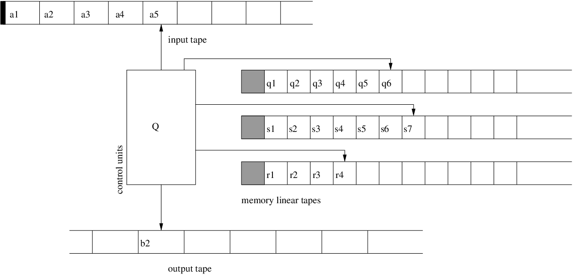
Let us briefly describe how such a machine operates. A move on a multistack machine $\mathcal{M}$ is based on :

$\bullet$

The current state of the finite control.
$\bullet$

The input symbol read.
$\bullet$

The top stack symbol on each of its stacks.

Based on these data, a move of the multistack machine consists in :

$\bullet$

Change the finite state control to a new state.
$\bullet$

For each stack, replace the top symbol by a (possibly empty) string of stack symbols. The choice of this string of symbols only depends on the input symbol read, the state of the finite control and on the top symbol of each stack.
$\bullet$

Move the head of the input tape to the right.

Remark 5.5.

Again, to make the machine deterministic, a move is uniquely determined by the knowledge of the input symbol read, the state of the finite control and on the top symbol of each stack.

As for pushdown automata, a multistack machine $\mathcal{M}$ can also possibly perform an $\epsilon$ -move : a move for which the head of the input tape does not move. The possibility of such a move depends only on the current state of the finite control and the top stack symbol on each of the stacks.

After reading a symbol of an input word $w$ , the finite state control of $\mathcal{M}$ could have reached a state $q$ from which $\epsilon$ -moves are still possible. In that case, we ask $\mathcal{M}$ to perform all possible $\epsilon$ -moves before reading the next input symbol. Also, a multistack machine is not allowed to stop its computation in a state from which an $\epsilon$ -move is possible.

After reading an input word $w$ , $\mathcal{M}$ produces a output symbol $a(w)$ that belongs to a finite output alphabet. The symbol $a(w)$ depends only on the state of the finite control and the top symbol of each stack. Given an integer $k\geq 2$ , a $k$ -multistack machine is a multistack machine that takes as input the base- $k$ expansion of an integer (that is, for which the input alphabet is $\Sigma_{k}$ ). In that case, the sequence $a(\langle n\rangle_{k})_{n\geq 0}$ is called the output sequence produced by $\mathcal{M}$ . With these definition, a deterministic $k$ -pushdown automata is nothing else than a $k$ -multistack machine with a single stack.

5.2.1 The Hartmanis–Stearns problem for stack-machines

One can now define the class of real numbers generated by multistack machines as follows.

Definition 5.6.

A real number $\xi$ can be generated by a $k$ -multistack machine $\mathcal{M}$ if, for some integer $b\geq 2$ , one has $\langle\{\xi\}\rangle_{b}=0.a_{1}a_{2}\cdots$ , where $(a_{n})_{n\geq 1}$ corresponds to the output sequence produced by $\mathcal{M}$ . A real number can be generated by a multistack machine if it can be generated by a $k$ -multistack machine for some $k$ .

Theorem 1.3 (resp. Theorem AB) can now be rephrased as follows : no algebraic irrational can be generated by a one-stack (resp. zero-stack) machine. Incidentally, this result turns out to provide a complete picture concerning the Hartmanis-Stearns problem for multistack machines. Indeed, since the two-stack machine has the same power as the general Turing machine, any computable number (and in particular any algebraic number) can be generated by a two-stack machine.

5.3 Beyond pushdown automata

We stress now that the equivalence relation $\sim$ given in Definition 4.4 and the associated Proposition 4.5 can be naturally extended to more general models of computation. For the multitape Turing machine, an internal configuration is determined by the state of the finite control and the complete knowledge of all the memory/working tapes (that is, the word written on each tape and the position of each head). But we do not need to concretely describe how the memory/working part of the machine is organized (tapes, stacks, or whatever). All what we need is to work with a machine with a one-way input tape and an output tape on which every symbol written is irrevocable. We refer to this kind of machines as one-way transducer-like machines. The Myhill-Nerode equivalence relation $\sim$ defined in 4.4 can be defined over the configurations of a one-way transducer-like machine : two configurations being equivalent if, starting from each configuration, there is no way to distinguish them by feeding the machine with arbitrary inputs. Moreover Proposition 4.5 also holds for these machines.

Proposition 5.7.

Let $\xi$ be a real number generated by a one-way transducer like machine. Let us assume that the equivalence relation $\sim$ is nontrivial in the sense that there exist two distinct positive integers $n$ and $n^{\prime}$ such that $C(n)\sim C(n^{\prime})$ . Then $\xi$ is either rational or transcendental.

This general result provides a method to prove the transcendence of real numbers which can be generated by machines more powerful than a $k$ -pushdown automata. For instance, it implies the transcendence of the ternary number

\xi_{3}:=0.110120110010110100101100110100110010110011010010112\dots

whose $n$ -th ternary digit is equal to $2$ if the binary expansion of $n$ is of the form $1^{k}0^{k}1^{k}$ , for some $k\in\mathbb{N}^{*}$ , to $1$ if the binary expansion of $n$ has a odd number of occurrences of ones, and to $0$ otherwise. This number cannot be generated by a $k$ -pushdown automaton because the set of words of the form $1^{k}0^{k}1^{k}$ , for some $k\in\mathbb{N}^{*}$ is not a context-free language. However, this language is context-sensitive which implies that $\xi_{3}$ can be generated by some kind of one-way transducer like machine (a linear bounded automaton). Proposition 5.7 can then be used to prove that $\xi_{3}$ is transcendental for one can show that $C(10)\sim C(20)$ for every one-way transducer-like machine generating $\xi_{3}$ .

6 Concluding remarks

We end this paper with several comments concerning factor complexity, transcendence measures, and continued fractions, also providing possible directions for further research.

6.1 Links with factor complexity

Another interesting way to tackle problems concerned with the expansions of classical constants in integer bases is to consider the factor complexity of real numbers. Let $\xi$ be a real number, $0\leq\xi<1$ , and $b\geq 2$ be a positive integer. Let us denote by ${\bf a}=(a_{n})_{n\geq 1}\in\Sigma_{b}^{\mathbb{N}}$ its base- $b$ expansion. The complexity function of $\xi$ with respect to the base $b$ is the function that associates with each positive integer $n$ the positive integer

p(\xi,b,n):=\mbox{Card}\{(a_{j},a_{j+1},\ldots,a_{j+n-1}),\;j\geq 1\}.

When $\xi$ does not belongs to $[0,1)$ , we just set $p(\xi,b,n):=p(\{\xi\},b,n)$ .

To obtain lower bounds for the complexity of classical mathematical constants remains a famous challenging problem. In this direction, the main result concerning algebraic numbers was obtained by Bugeaud and the first author [3] who proved that

\lim_{n\to\infty}\frac{p(\xi,b,n)}{n}=+\infty\,,

(6.1)

for all algebraic irrational numbers $\xi$ and all integers $b\geq 2$ . This lower bound implies Theorem AB for it is well-known that a real number generated by a finite automaton has factor complexity in $O(n)$ [27]. We stress that the situation is really different with pushdown automata and tag machines. Indeed, given a positive integer $d$ , there exist pushdown automata whose output sequence has a factor complexity growing at least like $n^{d}$ [36], while tag machines can output sequences with quadratic complexity (see for instance [38]). In particular, Theorems 1.2 and 1.3 do not follow from (). We now exemplify this difference by providing lower bounds for the complexity of the two numbers $\xi_{1}$ and $\xi_{2}$ defined in Sections 2.2 and 2.3.

6.1.1 A lower bound for $p(\xi_{1},3,n)$

It follows from the definition of the number $\xi_{1}$ that its ternary expansion is the fixed point of the morphism $\mu$ defined by $\mu(0)=021$ , $\mu(1)=012$ , $\mu(2)=2$ . We note that the letter $2$ has clearly bounded growth ( $|\mu^{n}(2)|=1$ for all $n\geq 0$ ) and that $\mu^{\omega}(0)$ contains arbitrarily large blocks of consecutive occurrences of the letter $2$ . Then, a classical result of Pansiot [38] implies that the complexity of the infinite word $\mu^{\omega}(0)$ is quadratic. In other words, one has :

c_{1}n^{2}<p(\xi_{1},3,n)<c_{2}n^{2}\,,

for some positive constants $c_{1}$ and $c_{2}$ .

6.1.2 A lower bound for $p(\xi_{2},2,n)$

Recall that the binary number $\xi_{2}$ is defined as follows : its $n$ -th binary digit is $1$ if the difference between the number of occurrences of the digits $0$ and $1$ in the binary expansion of $n$ is at most $1$ , and is $0$ otherwise. We outline a proof of the fact that

p(\xi_{2},2,n)=\Theta(n\log^{2}n)\,.

We can first infer from [32] that $p({\xi_{2}},2,n)=O(n(\log n)^{2})$ , for this sequence is generated by a pushdown automaton with only one ordinary stack symbol. In order to find a lower bound for $p({\xi_{2}},2,n)$ , we are going to describe a tag machine-like process (over an infinite alphabet) generating the binary expansion of $\xi_{2}$ . We first notice that another way to understand the action of the $2$ -PDA $\mathcal{A}$ in Figure 2.3 that generates the binary expansion of $\xi_{2}$ is to unfold it. This representation, given in Figure 6.1, corresponds to the transition graph of $\mathcal{A}$ : states in this graph are given by all possible configurations and transitions between configurations are just labelled by the input digits $0$ or $1$ . In Figure 6.1, the notation $qX^{n}$ means that, in this configuration, $\mathcal{A}$ is in state $q$ and the content of the stack is $XX\cdots X$ ( $n$ times).

-2,-3)(19,2.5) nclineq_0Ewq_0E nclineq_1Eq_1X naput[npos=.45] $1$ nclineq_1Xq_1E naput[npos=.45] $0$ nclineq_1Xq_1X2 naput[npos=.45] $1$ nclineq_1X2q_1X naput[npos=.45] $0$ nclineq_1X2q_1X3 naput[npos=.45] $1$ nclineq_1X3q_1X2 naput[npos=.45] $0$ nclineq_1X3q_1X4 naput[npos=.45] $1$ nclineq_1X4q_1X3 naput[npos=.45] $0$ nclineq_1X4q_1X5 naput[npos=.45] $1$ nclineq_1X5q_1X4 naput[npos=.45] $0$ nclineq_1X5q_1s naput[npos=.45] $1$ nclineq_1sq_1X5 naput[npos=.45] $0$ nclineq_1Eq_0E naput[npos=.45] $0$ nclineq_0Eq_1E naput[npos=.45] $1$ nclineq_0ErE naput[npos=.45] $0$ nclinerEq_0E naput[npos=.45] $1$ nclinerErX naput[npos=.45] $0$ nclinerXrE naput[npos=.45] $1$ nclinerXrX2 naput[npos=.45] $0$ nclinerX2rX naput[npos=.45] $1$ nclinerX2rX3 naput[npos=.45] $0$ nclinerX3rX2 naput[npos=.45] $1$ nclinerX3rX4 naput[npos=.45] $0$ nclinerX4rX3 naput[npos=.45] $1$ nclinerX4rX5 naput[npos=.45] $0$ nclinerX5rX4 naput[npos=.45] $1$ nclinerX5rs naput[npos=.45] $0$ nclinersrX5 naput[npos=.45] $1$

Figure 6.1: The transition graph of

\mathcal{A}

In Figure 6.2, states of the transition graph has been renamed as follows : configurations are replaced with integers, where reading a $1$ in state $n$ leads to a move to state $n+1$ and reading a $0$ in state $n$ leads to a move to state $n-1$ . We easily see that the output state is just the difference between the number of $1$ ’s and $0$ ’s in the input word. Thus the $n$ -th binary digit of $\xi_{2}$ is equal to $1$ if and only if the reading of the binary expansion of $n$ by this infinite automaton ends in one of the three states labelled by $0$ , $-1$ and $1$ .

-2,-3)(19,2.5) nclineqEwqE nclinepEpX naput[npos=.45] $1$ nclinepXpE naput[npos=.45] $0$ nclinepXpX2 naput[npos=.45] $1$ nclinepX2pX naput[npos=.45] $0$ nclinepX2pX3 naput[npos=.45] $1$ nclinepX3pX2 naput[npos=.45] $0$ nclinepX3pX4 naput[npos=.45] $1$ nclinepX4pX3 naput[npos=.45] $0$ nclinepX4pX5 naput[npos=.45] $1$ nclinepX5pX4 naput[npos=.45] $0$ nclinepX5ps naput[npos=.45] $1$ nclinepspX5 naput[npos=.45] $0$ nclinepEqE naput[npos=.45] $0$ nclineqEpE naput[npos=.45] $1$ nclineqErE naput[npos=.45] $0$ nclinerEqE naput[npos=.45] $1$ nclinerErX naput[npos=.45] $0$ nclinerXrE naput[npos=.45] $1$ nclinerXrX2 naput[npos=.45] $0$ nclinerX2rX naput[npos=.45] $1$ nclinerX2rX3 naput[npos=.45] $0$ nclinerX3rX2 naput[npos=.45] $1$ nclinerX3rX4 naput[npos=.45] $0$ nclinerX4rX3 naput[npos=.45] $1$ nclinerX4rX5 naput[npos=.45] $0$ nclinerX5rX4 naput[npos=.45] $1$ nclinerX5rs naput[npos=.45] $0$ nclinersrX5 naput[npos=.45] $1$

Figure 6.2: Relabelling of the transition graph of

\mathcal{A}

The action of $0$ and $1$ can be summarized by $n\xrightarrow{0}n-1$ and $n\xrightarrow{1}n+1$ . This leads to a tag machine-like process over an infinite alphabet $\mathcal{T}=(A,\sigma,s,B,\varphi)$ for generating the expansion of $\xi_{2}$ . The starting symbol is $s$ , $A=\mathbb{Z}\cup\{s\}$ , $\sigma$ is defined by $\sigma(s)=s1$ and $\sigma(n)=(n-1)(n+1)$ , $B=\{0,1\}$ , $\varphi(-1)=\varphi(0)=\varphi(1)=1$ , and $\varphi(e)=0$ if $e\notin\{s,-1,0,1\}$ . Then we have $\langle\xi\rangle_{2}=0.\varphi(\sigma^{\omega}(s))$ , where the infinite word

\sigma^{\omega}(s)=s\,1\,0\,2\,(-1)\,1\,1\,3\,(-2)\,0\,0\,2\,0\,2\,2\,4\,(-3)\,(-1)\,(-1)\,1\,(-1)\,1\,1\,3\,(-1)\,1\,1\cdots

is the unique fixed point of the morphism $\sigma$ .

The strategy consists now in finding sufficiently many different right special factors, that is factors $w$ of $\varphi(\sigma^{\omega}(s))$ for which both factors $w0$ and $w1$ also occur in $\varphi(\sigma^{\omega}(s))$ . Arguing as in [31, Lemma 1.13], one can actually show that, for every pair

(p,q)\in{\mathcal{E}}:=\{(p,q)\in\mathbb{N}^{2}\mid 1\leq p\leq q\leq k-2\}\,,

both words

A:=\varphi(\sigma^{k}(k-2p)\sigma^{k}(k-2p+2)\sigma^{k}(k-2q))

and

B:=\varphi(\sigma^{k}(k-2p)\sigma^{k}(k-2p+2)\sigma^{k}(-k-2))

occur in $\varphi(\sigma^{\omega}(s))$ and they have the same factor of length $n$ , say $w(p,q)$ , occurring at index $2^{k+1}+2^{q}-n$ . Furthermore, in the word $A$ the factor $w(p,q)$ is followed by a $1$ , while in the word $B$ it is followed by a $0$ . Thus $w(p,q)$ is a right special factor. It can also be extracted from [31, Lemma 1.13] that the map $(p,q)\mapsto w(p,q)$ is injective on $\mathcal{E}$ . This ensures the existence of at least $\frac{(k-2)(k-1)}{2}$ distinct right special factors of length $n$ in $\varphi(\sigma^{\omega}(s))$ . Then it follows that

p(\xi_{2},2,n+1)-p(\xi_{2},2,n)\geq\frac{(k-2)(k-1)}{2}\,,

from which one easily deduces the lower bound :

p({\xi_{2}},2,n)\geq cn(\log n)^{2}\,,

for some positive constant $c$ .

6.2 Quantitative aspects : transcendence measures and the imitation game

We discuss here some problems related to the quantitative aspects of our results.

6.2.1 The number theory side : transcendence measures

A real number $\xi$ is transcendental if $|P(\xi)|>0$ , for all non-zero integer polynomials $P(X)$ . A transcendence measure for $\xi$ consists in a limitation of the smallness of $|P(\xi)|$ , thus refining the transcendence statement. In general, one looks for a nontrivial function $f$ satisfying :

|P(\xi)|>f(H,d)\,,

for all integer polynomials of degree at most $d$ and height at most $H$ . Here, $H(P)$ stands for the naïve height of the polynomial $P(X)$ , that is, the maximum of the absolute values of its coefficients. The degree and the height of an integer polynomial $P$ allow to take care of the complexity of $P$ . We will use here the following classification of real numbers defined by Mahler [33] in 1932. For every integer $d\geq 1$ and every real number $\xi$ , we denote by $w_{d}(\xi)$ the supremum of the exponents $w$ for which

0<|P(\xi)|<H(P)^{-w}

has infinitely many solutions in integer polynomials $P(X)$ of degree at most $d$ . Further, we set $w(\xi)=\limsup_{d\to\infty}(w_{d}(\xi)/d)$ and, according to Mahler [33], we say that $\xi$ is an

A

-number, if

w(\xi)=0

;

S

-number, if

0<w(\xi)<\infty

;

T

-number, if

w(\xi)=\infty

and

w_{d}(\xi)<\infty

for any integer

d\geq 1

;

U

-number, if

w(\xi)=\infty

and

w_{d}(\xi)=\infty

for some integer

d\geq 1

An important feature of this classification is that two transcendental real numbers that belong to different classes are algebraically independent. The $A$ -numbers are precisely the algebraic numbers and, in the sense of the Lebesgue measure, almost all numbers are $S$ -numbers.

A Liouville number is a real number $\xi$ such that for any positive real number $\rho$ the inequality

\left|\xi-\frac{p}{q}\right|<\frac{1}{q^{\rho}}

has a at least one solution $(p,q)\in\mathbb{Z}^{2}$ , with $q>1$ . Thus $\xi$ is a Liouville number if, and only if, $w_{1}(\xi)=+\infty$ .

Let $\xi$ be an irrational real number defined through its base- $b$ expansion, say $\langle\{\xi\}\rangle_{b}:=0.a_{1}a_{2}\cdots$ . Let us assume that the base- $b$ expansion of $\xi$ can be generated either by a pushdown automata or by a tag machine with dilation factor larger than one. As recalled in Proposition ABL (Section 3), the key point for proving that $\xi$ is transcendental is to show that ${\rm dio}({\bf a})>1$ , where ${\bf a}:=a_{1}a_{2}\cdots$ . This comes down to finding two sequences of finite words $(U_{n})_{n\geq 0}$ and $(V_{n})_{n\geq 0}$ , a sequence of rational numbers $\alpha_{n}$ , and a real number $\delta>0$ such that the word $U_{n}V_{n}^{\alpha_{n}}$ is a prefix of ${\bf a}$ , the length of the word $U_{n}V_{n}^{\alpha_{n}}$ increases, and

\frac{|U_{n}V_{n}^{\alpha_{n}}|}{|U_{n}V_{n}|}\geq 1+\delta\,.

(6.2)

A look at the proofs of Theorems 1.2 and 1.3 show that one actually has, in both cases, the following extra property : there exists a real number $M$ such that

\limsup_{n\to\infty}\frac{|U_{n+1}V_{n+1}|}{|U_{n}V_{n}|}<M\,.

(6.3)

Using an approach introduced in [9] and developed in [6], one can first prove that

{\rm dio}({\bf a})-1\leq w_{1}(\xi)\leq c_{1}{\rm dio}({\bf a})\,,

(6.4)

for some real number $c_{1}$ that depends only on $\delta$ and $M$ . In particular, $\xi$ is a Liouville number if and only if ${\rm dio}({\bf a})$ is infinite. Then it is proved in [6], following a general approach introduced in [5] and based on a quantitative version of the subspace theorem, that this extra condition leads to transcendence measures. Indeed, taking all parameters into account, one could derive an upper bound of the type

w_{d}(\xi)\leq\max\{w_{1}(\xi),(2d)^{c_{2}(\log 3d)(\log\log 3d)}\}\,,

(6.5)

for all positive integers $d$ and some real number $c_{2}$ that depends only on $\delta$ and $M$ . The constants $c_{1}$ and $c_{2}$ can be made effective. In particular, we deduce from Inequalities (6.4) and (6.5) the following result.

Theorem 6.1.

Let $\xi$ be an irrational real number such that $\langle\{\xi\}\rangle_{b}:=0.a_{1}a_{2}\cdots$ and let ${\bf a}:=a_{1}a_{2}\cdots$ . Let us assume that the base- $b$ expansion of $\xi$ can be generated either by a pushdown automata or by a tag machine with dilation factor larger than one. Then one of the following holds.

(i)

${\rm dio}({\bf a})=+\infty$ and $\xi$ is a Liouville number.
(ii)

${\rm dio}({\bf a})<+\infty$ and $\xi$ is a $S$ - or a $T$ -number.

Of course, in view of Theorem 6.1, it would be interesting to prove whether or not there exist such numbers for which ${\rm dio}({\bf a})=+\infty$ . In this direction, it is proved in [9] that ${\rm dio}({\bf a})$ is always finite when $\xi$ is generated by a finite automaton. We add here the following contribution to this problem.

Proposition 6.2.

Let ${\bf a}:=a_{1}a_{2}\cdots$ be an aperiodic purely morphic word generated by a morphism $\sigma$ defined over a finite alphabet $A$ . Set $M:=\max\{|\sigma(i)|\mid i\in A\}$ . Then ${\rm dio}({\bf a})\leq M+1$ .

Démonstration.

Let us assume that $\sigma$ is prolongable on the letter $a$ and that $\sigma^{\omega}(a)=a_{1}a_{2}\cdots$ . We argue now by contradiction by assuming that ${\rm dio}({\bf a})>M+1$ .

This assumption ensures that one can find two finite words $U$ and $V$ and a real number $s>1$ such that :

(i)

$UV^{s}$ is a prefix of ${\bf a}$ , and $s$ is maximal with this property.
(ii)

One has

$|UV^{s}|/|UV|\geq M+1\,.$
(iii)

$V$ is primitive (i.e. is non-empty and not the integral power of a shorter word) and $s$ is maximal.

Not that since ${\bf a}$ is fixed by $\sigma$ then the word $\sigma(UV^{s})$ is also a prefix of ${\bf a}$ . By definition of $M$ , it follows from (ii) that

UV^{s}=\sigma(U)W\,,

where $W=\widetilde{V}^{\alpha}$ for some conjugate $\widetilde{V}$ of $V$ (i.e., $V=AB$ and $\widetilde{V}=BA$ for some $A,B$ ) and $\alpha\leq s$ . On the other hand, $\sigma(V)$ is also a period of $W$ since $UV^{s}=\sigma(U)W$ is a prefix of $\sigma(UV^{s})=\sigma(U)\sigma(V)^{s^{\prime}}$ , for some $s^{\prime}$ . Thus $W$ has at least two periods : $\widetilde{V}$ and $\sigma(V)$ . Furthermore, (ii) implies that

|UV^{s-1}|\geq M(|U|+|V|)

and then

|W|=|UV^{s}|-|\sigma(U)|\geq|\sigma(V)|+|V|=|\sigma(V)|+|\widetilde{V}|\,.

We can thus apply Fine and Wilf’s theorem (see for instance [12, Chap. 1]) to the word $W$ and we obtain that there is a word of length $\gcd(|\widetilde{V}|,|\sigma(V)|)$ that is a period of $W$ . But, since $V$ is primitive, the word $\widetilde{V}$ is primitive too, and it follows that $\gcd(|\widetilde{V}|,|\sigma(V)|)=|\widetilde{V}|$ . This gives that $\sigma(V)=\widetilde{V}^{k}$ for some positive integer $k$ . It follows that

\sigma(UV^{s})=\sigma(U)\widetilde{V}^{ks^{\prime}}=UV^{s-\alpha+ks^{\prime}}

is a prefix of ${\bf a}$ . Now the inequality $|\sigma(UV^{s})|>|UV^{s}|$ gives a contradiction with the maximality of $s$ . This ends the proof. ∎

6.2.2 The computer science side : the imitation game

Theorems AB, 1.2, and 1.3 show that some classes of Turing machines are too limited to produce the base- $b$ expansion of an algebraic irrational real number. Let $\xi$ be an irrational real number that can be generated by a $k$ -pushdown automaton or by a tag machine with dilation factor larger than one. Then the results of Section 6.2 could be rephrased to provide a limitation of the way $\xi$ can be approximated by irrational algebraic numbers. In this section, we suggest to view things from a different angle, changing our target. Indeed, we fix an algebraic irrational real number $\alpha$ and a base $b$ , and ask for how long the base- $b$ expansion of $\alpha$ can be imitated by outputs of a given class of Turing machines.

Let us explain now how to formalize our problem. We can naturally take the number of states as a measure of complexity of a $k$ -automaton. One can also defined the size of $k$ -pushdown automata and tag machines as follows. Let us define the size of a $k$ -pushdown automaton $\mathcal{A}:=(Q,\Sigma_{k},\Gamma,\delta,q_{0},\Delta,\tau)$ to be $|Q|+|\Gamma|+L$ , where $L$ is the maximal length of a word that can be added to the stack by the transition function $\delta$ of $\mathcal{A}$ . Let us also define the size of a tag machine $\mathcal{T}:=(A,\sigma,a,\varphi,B)$ to be $|A|+L$ , where $L:=\max\{|\sigma(i)|\mid i\in A\}$ . Now, let us fix a class $\mathcal{M}$ of Turing machines among $k$ -automata, $k$ -pushdown automata, and tag machines. Let $M$ be a positive integer. We stress that there are only finitely many such machines with size at most $M$ . Then there exists a maximal positive integer $I(\alpha,M)$ for which there exists a machine in $\mathcal{M}$ with size at most $M$ whose output agrees with the base- $b$ expansion of $\alpha$ at least up to the $I(\alpha,M)$ -th digit. We suggest the following problem.

Problem 6.3.

Let $\alpha$ be an algebraic irrational real number and fix a class of Turing machines among $k$ -automata, $k$ -pushdown automata, and tag machines. Given a positive integer $M$ , find an upper bound for $I(\alpha,M)$ .

In the case of finite automata, we can give a first result toward this problem. Indeed, the factor complexity of the output ${\bf a}$ of a $k$ -automaton with at most $M$ states satisfies $p({\bf a},n)\leq kM^{2}n$ (see for instance [12]). Let us denote respectively by $d$ and $H$ the degree and the height of $\alpha$ . Then the main result of [19] allows to extract the following upper bound :

	$\displaystyle I(\alpha,M)$	$\displaystyle\leq$	$\displaystyle\max\left\{(\max(\log H,e)100kM^{2})^{8\log 4kM^{2}}\right.,$
			$\displaystyle\;\;\;\;\;\;\;\;\;\;\;\;\left.\left((\log d)10^{100}(kM^{2})^{11/2}\log(kM^{2})\right)^{2.1}\right\}\,.$

6.3 Computational complexity of the continued fraction expansion of algebraic numbers

Replacing integer base expansions with continued fractions leads to similar problems. Rational numbers all have a finite continued fraction expansion, while quadratic real numbers correspond to eventually periodic continued fractions. In contrast, much less is known about the continued fraction expansion of algebraic real numbers of degree at least three such as $\sqrt[3]{2}$ . In this direction, an approach based on the subspace theorem was introduced by Bugeaud and the first author [2]. Recently, Bugeaud [20] shows that this approach actually leads to the following analogue of Proposition ABL.

Proposition B. — Let $\xi$ be a real number with $\xi:=[a_{0},a_{1},a_{2},\ldots]$ where we assume that $(a_{n})_{n\geq 1}$ is a bounded sequence of positive integers. Let us assume that ${\rm dio}({\bf a})>1$ where ${\bf a}:=a_{1}a_{2}\cdots$ . Then $\xi$ is either quadratic or transcendental.

In [20], the author deduce from Proposition B that the continued fraction expansion of an algebraic real number of degree at least $3$ cannot be generated by a finite automaton. This provides the analogue of Theorem AB in this framework. As a direct consequence of our results and Proposition B, we obtain the following generalization of Bugeaud’s result corresponding to the analogue of Theorems 1.2 and 1.3.

Theorem 6.4.

Let $\xi$ be an algebraic real number of degree at least $3$ . Then the following holds.

(i)

The continued fraction expansion of $\xi$ cannot be generated by a one-stack machine, or equivalently, by a deterministic pushdown automaton.
(ii)

The continued fraction expansion of $\xi$ cannot be generated by a tag machine with dilation factor larger than one.

Using the approach introduced in [7] and the discussion of Section 6.2, it will also be possible to produce transcendence measures analogous to Theorem 6.1 for real numbers whose continued fraction expansion can be generated by deterministic pushdown automata or by a tag machine with dilation factor larger than one.

Références

[1] B. Adamczewski, On the expansion of some exponential periods in an integer base, Math. Ann. 346 (2010), 107–116.
[2] B. Adamczewski and Y. Bugeaud, On the complexity of algebraic numbers II. continued fractions, Acta Math. 195 (2005), 1–20.
[3] B. Adamczewski and Y. Bugeaud, On the complexity of algebraic numbers I. Expansions in integer bases, Ann. of Math. 165 (2007), 547–565.
[4] B. Adamczewski and Y. Bugeaud, Dynamics for $\beta$ -shifts and Diophantine approximation, Ergod. Th. & Dynam. Sys. 27 (2007), 1695–1710.
[5] B. Adamczewski and Y. Bugeaud, Mesures de transcendance et aspects quantitatifs de la méthode de Thue-Siegel-Roth-Schmidt, Proc. London Math. Soc. 101 (2010), 1–31.
[6] B. Adamczewski and Y. Bugeaud, Nombres réels de complexité sous-linéaire : mesures d’irrationalité et de transcendance, J. Reine Angew. Math. 658 (2011), 65–98.
[7] B. Adamczewski and Y. Bugeaud, Trancendence measure for continued fractions involving repetitive or symmetric patterns, J. Eur. Math. Soc. 12 (2010), 883–914.
[8] B. Adamczewski, Y. Bugeaud and F. Luca, Sur la complexité des nombres algébriques, C. R. Acad. Sci. paris 339 (2004), 11–14.
[9] B. Adamczewski and J. Cassaigne, Diophantine properties of real numbers generated by finite automata, Compos. Math. 142 (2006), 1351–1372.
[10] B. Adamczewski and C. Faverjon, Méthode de Mahler : relations linéaires, transcendance et applications aux nombres automatiques, Proc. London Math. Soc. 115 (2017), 55–90.
[11] J. Albert, Propriétés combinatoires et arithmétiques de certaines suites automatiques et substitutives, Thèse de Doctorat de l’Université Paris Sud, 2006.
[12] J.-P. Allouche and J. Shallit, Automatic sequences. Theory, applications, generalizations, Cambridge University Press, Cambridge, 2003.
[13] J.-M. Autebert, Langages algébriques, Études et Recherches en Informatique, Masson, Paris, 1987.
[14] J.-M. Autebert, J. Berstel, and L. Boasson, Context-free languages and push-down automata, in Handbook of formal languages, pp. 111-174, Springer, 1997.
[15] J. Berstel et L. Boasson, Modèles de machines, in Encyclopédie de l’informatique et des systèmes d’information, pp. 987–998, Vuibert, 2006.
[16] D. Bertrand, Theta functions and transcendence, Ramanujan J. 1 (1997), 339–350.
[17] É. Borel, Les probabilités dénombrables et leurs applications arithmétiques, Rend. Circ. Mat. Palermo 27 (1909), 247–271.
[18] J. M. Borwein and P. B. Borwein, On the complexity of familiar functions and numbers, SIAM Rev. 30 (1988), 589–601.
[19] Y. Bugeaud, An explicit lower bound for the block complexity of an algebraic number, Atti Accad. Naz. Lincei Cl. Sci. Fis. Mat. Natur. Rend. Lincei (9) Mat. Appl. 19 (2008), 229–235.
[20] Y. Bugeaud, Automatic continued fractions are transcendental or quadratic, Ann. Sci. École Norm. Sup. 46 (2013), 1005–1022.
[21] J. Cassaigne and F. Nicolas, Factor complexity, in Combinatorics, automata and number theory, Encyclopedia Math. Appl. 135, pp. 163–247, Cambridge Univ. Press, Cambridge, 2010.
[22] D. Caucal and M. Le Gonidec, Context-free automatic sequences, in Procceding of Theoretical Aspects of Computing - ICTAC 2014, pp. 259–276, 2014.
[23] N. Chomsky, Three models for the description of language, IRE Trans. Information Theory (1956), 113–124.
[24] A. Cobham, Functional equations for register machines, in Proccedings of the Hawaii International Conference on System Sciences, Honolulu, 1968.
[25] A. Cobham, A proof of transcendence based on functional equations, RC–2041, IBM Research Center, Yorktown Heights, New York, 1968.
[26] A. Cobham, On the Hartmanis-Stearns problem for a class of tag machines, in IEEE Conference Record of 1968 Ninth Annual Symposium on Switching and Automata Theory, pp. 51–60, 1968.
[27] A. Cobham, Uniform tag sequences, Math. Systems Theory 6 (1972), 164–192.
[28] D. Duverney, Ke. Nishioka, Ku. Nishioka, I. Shiokawa, Transcendence of Jacobi’s theta series. Proc. Japan Acad. Sci. 72 (1996), 202–203.
[29] J. Hartmanis and R. E. Stearns, On the computational complexity of algorithms, Trans. Amer. Math. Soc. 117 (1965), 285–306.
[30] J. E. Hopcroft, R. Motawi and J. D. Ullman, Introduction to automata theory, languages, and computation, third edition, Prentice Hall, 2006.
[31] M. Le Gonidec, Drunken man infinite words complexity, RAIRO - Theoret. Inf. and Appl. 42 (2008), 599–613.
[32] M. Le Gonidec, On the complexity of a family of $k$ -context-free sequences, Theoret. Comp. Sci. 44 (2012), 47–54.
[33] K. Mahler, Zur Approximation der Exponentialfunktionen und des Logarithmus. I, II, J. reine angew. Math. 166 (1932), 118–150.
[34] M. L. Minsky, Computation : finite and infinite machines, Prentice-Hall Series in Automatic Computation, New Jersey, 1967.
[35] M. Morse and G. A. Hedlund, Symbolic dynamics, Amer. J. Math. 60 (1938), 815–866.
[36] Y. Moshe, On some questions regarding $k$ -regular and $k$ -context-free sequences, Theoret. Comput. Sci. 400 (2008), 62–69.
[37] Yu. V. Nesterenko, Modular functions and transcendence problems, Math. Sb. 187 (1996), 65–96.
[38] J.-J. Pansiot, Complexité des facteurs des mots infinis engendrés par morphismes itérés, in : Automata, languages and programming (Antwerp, 1984), 380–389, Lecture Notes in Comput. Sci. 172, Springer, 1984.
[39] P. Philippon, Groupes de Galois et nombres automatiques, J. Lond. Math. Soc. 92 (2015), 596–614.
[40] N. Pytheas Fogg, Substitutions in dynamics, arithmetics and combinatorics, Lecture Notes in Math. 1794, Springer-Verlag, Berlin, 2002.
[41] M. Queffélec, Substitution dynamical systems–spectral analysis (second edition), Lecture Notes in Math. 1294. Springer-Verlag, Berlin, 2010.
[42] M. Sipser, Introduction to the theory of computation, third edition, Wadsworth Publishing Co. Inc., 2012.
[43] A. M. Turing, On computable numbers, with an application to the Entscheidungsproblem, Proc. London Math. Soc. 42 (1937), 230–265 ; corrigendum 43 (1937) 544–546.

On the computational complexity of algebraic numbers : the Hartmanis–Stearns problem revisited

Résumé

1 Introduction

Remark 1.1.

Theorem 1.2 (Cobham’s second claim).

Theorem 1.3.

2 Finite automata, morphic sequences and pushdown automata

2.1 Finite automata and automatic sequences

Definition 2.1.

Example 2.2.

Definition 2.3.

2.2 Morphic sequences

Definition 2.4.

Definition 2.5.

Remark 2.6.

Example 2.7.

2.3 Pushdown automata

Remark 2.8.

Definition 2.9.

Example 2.10.

Definition 2.11.

Remark 2.12.

3 A combinatorial transcendence criterion

Definition 3.1.

4 Proof of Theorems 1.2 and 1.3

4.1 Proof of Theorem 1.2

Definition 4.1.

Lemma 4.2.

Démonstration.

Proposition 4.3.

Démonstration.

Proof of Theorem 1.2.

4.2 Proof of theorem 1.3

Definition 4.4.

Proposition 4.5.

Démonstration.

Proof of Theorem AB.

Proof of Theorem 1.3.

5 Some related models of computations : tag machines and stack machines

5.1 Tag-machines

Definition 5.1.

Definition 5.2.

Remark 5.3.

Proposition 5.4.

Démonstration.

5.2 Pushdown automata viewed as multistack machines

Remark 5.5.

5.2.1 The Hartmanis–Stearns problem for stack-machines

Definition 5.6.

5.3 Beyond pushdown automata

Proposition 5.7.

6 Concluding remarks

6.1 Links with factor complexity

6.1.1 A lower bound for p⁡(ξ1​,3,n)p(\xi_{1},3,n)

6.1.2 A lower bound for p⁡(ξ2​,2,n)p(\xi_{2},2,n)

6.2 Quantitative aspects : transcendence measures and the imitation game

6.2.1 The number theory side : transcendence measures

Theorem 6.1.

Proposition 6.2.

Démonstration.

6.2.2 The computer science side : the imitation game

Problem 6.3.

6.3 Computational complexity of the continued fraction expansion of algebraic numbers

Theorem 6.4.

Références

6.1.1 A lower bound for $p(\xi_{1},3,n)$

6.1.2 A lower bound for $p(\xi_{2},2,n)$