Number of trials required to estimate a free-energy difference,
using fluctuation relations

The numerical estimation of free-energy differences is an active area of research, having applications to chemistry, microbiology, pharmacology, and other fields. Fluctuation relations can be used to estimate equilibrium free-energy differences $\Delta F$ from nonequilibrium experimental and simulation data. One repeatedly measures the amount $W$ of work extracted from, or performed on, a system during an experiment or simulation. Fluctuation relations express the value of $\Delta F$ in terms of averages over infinitely many trials. Finitely many trials are performed in practice, introducing errors into estimates of $\Delta F$. Efforts to quantify these errors, and to promote “good practices” in estimating $\Delta F$, have been initiated (e.g., [1, 2, 3, 4, 5, 6, 7, 8, 9, 10, 11, 12]).

How many trials should one perform to estimate $\Delta F$ reliably? The work $W$ extracted from a system is a random variable that assumes different values in different trials. Typical trials involve $W$-values that contribute little to the averages being estimated. Dominant $W$-values, which largely determine the averages, characterize few trials [13]. Until observing a dominant $W$-value, one cannot estimate $\Delta F$ with reasonable accuracy. The probability that some trial will involve a dominant $W$-value determines the number $N$ of trials one should expect to perform.

A rough estimate of $N$ was provided in [13]. In this paper, we enhance the estimate’s precision. First, we introduce fluctuation relations and one-shot information theory, a mathematical toolkit for quantifying efficiencies at small scales. Next, we quantify dominance in terms of a tolerance parameter $w^{\delta}$. We bound the number $N_{\delta}$ of trials expected to be required to observe a dominant work value. This bound depends on the thermal order-$\infty$ Rényi entropy $H^{\beta}_{\infty}$, a quantity inspired by one-shot information theory [14]. The bound can be estimated during an implementation of the “bidirectionality good practice” recommended in [1]. Finally, we approximately bound the error in a $(\Delta F)$-estimate inferred from $N_{\delta}$ trials. A weakly interacting dilute classical gas [15] illustrates our analytical results.

Technical introduction—Let us introduce nonequilibrium fluctuation relations and the thermal order-$\infty$ Rényi entropy $H^{\beta}_{\infty}$.

Nonequilibrium fluctuation relations—Nonequilibrium fluctuation relations govern statistical mechanical systems arbitrarily far from equilibrium. Consider a system in thermal equilibrium with a heat bath at inverse temperature $\beta\equiv\frac{1}{k_{\rm B}T}$, wherein $k_{\rm B}$ denotes Boltzmann’s constant. We focus on classical systems for simplicity, though fluctuation relations have been extended to quantum systems [16]. Suppose that a time-dependent external parameter $\lambda_{t}$ determines the system’s Hamiltonian: $H=H(\lambda_{t},\mathbf{z})$, wherein $\mathbf{z}$ denotes a phase-space point. If the system consists of an ideal gas in a box, $\lambda_{t}$ may denote the height of the piston that caps the gas. Suppose that, at time $t=-\tau$, the system begins with the equilibrium phase-space density $e^{-\beta H(\lambda_{-\tau},\mathbf{z})}/Z_{-\tau}$, wherein the partition function $Z_{-\tau}$ normalizes the state. The external parameter is then varied according to a predetermined schedule $\lambda_{t}$, from $t=-\tau$ to $t=\tau$. The system evolves away from equilibrium if $\tau$ is finite. In the gas example, the piston is lowered, compressing the gas. We call this process the forward protocol.

The reverse protocol begins with the system at equilibrium relative to $H(\lambda_{\tau},\mathbf{z})$. The external parameter is changed to $\lambda_{-\tau}$ along the time-reverse of the path followed during the forward protocol. In the gas example, the piston is raised, and the gas expands.

Changing the external parameter requires or outputs some amount of work. We use the following sign convention: The forward process tends to require an investment of a positive amount $W>0$ of work, and the reverse process tends to output $W>0$. The value of $W$ varies from trial to trial. After performing many trials, one can estimate the probability $P_{\mathrm{fwd}}(W)$ that any particular forward trial will cost an amount $W$ of work and the probability $P_{\mathrm{rev}}(-W)$ that any particular reverse trial will output an amount $W$.

These probabilities satisfy Crooks’ Theorem [17],

Here, $\Delta F:=F_{\tau}-F_{-\tau}$ denotes the difference between the free energy $F_{\tau}=-\beta^{-1}\log(Z_{\tau})$ of the Gibbs distribution $e^{-\beta H(\lambda_{\tau},\mathbf{z})}/Z_{\tau}$ corresponding to the final Hamiltonian and the free energy $F_{-\tau}=-\beta^{-1}\log(Z_{-\tau})$ of the Gibbs distribution corresponding to $H(\lambda_{-\tau},\mathbf{z})$. Multiplying each side of Crooks’ Theorem by $P_{\mathrm{rev}}(-W)e^{\beta\Delta F}$, then integrating over $W$, yields a version of the nonequilibrium work relation [18]:

The angle brackets denote an average over infinitely many trials. To calculate $\Delta F$, one performs many trials, estimates the average, and substitutes into Eq. (2).

Thermal order-$\infty$ Rényi entropy ($H^{\beta}_{\infty}$)—Entropies quantify uncertainties in statistical mechanics and in information theory. Let $P:=\{p_{i}\}$ denote a probability distribution over a discrete random variable $X$. The Shannon entropy $H_{S}(P):=-\sum_{i}p_{i}\log(p_{i})$ quantifies an average, over infinitely many trials, of the information one gains upon learning the value assumed by $X$ in one trial [19].

$H_{S}$ has been generalized to a family of Rényi entropies $H_{\alpha}$. The parameter $\alpha\in[0,\infty)$ is called the order. The $H_{\alpha}$’s quantify uncertainties related to finitely many trials. In the limit as $\alpha\to\infty$, $H_{\alpha}$ approaches

wherein $p_{\rm max}$ denotes the greatest $p_{i}$. This maximal entropy has applications to randomness extraction: The efficiency with which finitely many copies of $P$ can be converted into a uniformly random distribution $(\underbrace{\frac{1}{d},\ldots,\frac{1}{d}}_{d})$ is quantified with $H_{\infty}(P)$ [20].

The distributions $P_{\mathrm{fwd}}$ and $P_{\mathrm{rev}}$ in Crooks’ Theorem are continuous. Hence we need a continuous analog of $H_{\infty}$. The definition

has been shown to be useful in contexts that involve heat baths [14]. $p_{\rm max}$ denotes the greatest value of the probability density $P$. $p_{\rm max}$ can diverge, e.g., if $P$ represents a Dirac delta function. But delta functions characterize the work distributions of quasistatic protocols, whose work $W=\Delta F$ in every trial. We focus on more-realistic, quick protocols. $P_{\mathrm{fwd}}$ and $P_{\mathrm{rev}}$ are short and broad, so $p_{\rm max}$ is finite.

The density $p_{\rm max}$ has dimensions of inverse energy, which are canceled by the $\beta$ in Eq. (5). Hence the logarithm’s argument is dimensionless. For further discussion about $H^{\beta}_{\infty}$, see [14].

Quantification of dominance—Let us return to the nonequilibrium work relation (3). The exponential enlarges already-high $W$-values, which dominate the integral. To estimate the integral accurately, one must perform trials that output large amounts of work. Few trials do; dominant $W$-values are atypical [13]. How many trials should one expect to need to perform, to achieve reasonable convergence of the exponential average in Eq. (3)?

An approximate answer was provided in [13]:

wherein $\langle.\rangle_{\mathrm{fwd}}$ denotes an average with respect to $P_{\mathrm{fwd}}(W)$. The average dissipated work $\langle W\rangle_{\mathrm{fwd}}-\Delta F$ represents the mean amount of work wasted as heat. Switching $\lambda_{t}$ quasistatically (infinitely slowly) would cost an amount $\Delta F$ of work. Switching at a finite speed costs more: Work is dissipated into the bath as heat when the system is driven away from equilibrium. The dissipated work $W-\Delta F$ signifies the extra work paid to switch $\lambda_{t}$ in a finite amount of time.

How large must a $W$-value be to qualify as dominant? This question remained open in [13]. We propose a definition inspired by information-theoretic protocols in which an agent specifies an error tolerance. The experimenter who switches $\lambda_{t}$, or the programmer who simulates trials, chooses a threshold value of $w^{\delta}$ used to lower-bound the $W$-values considered large.

A similar quantity is defined in [3]. Lu and Kofke assess the accuracy of free-energy-perturbation (FEP) calculations. FEP is used to estimate free-energy differences $\Delta F$. FEP results from a limit of nonequilibrium-fluctuation theory [18]. In [3], a fixed-length simulation is assumed to be performed. A difference $u$ between potential energies is measured. $u$, in FEP, plays the role of $W$ in nonequilibrium fluctuation relations. Lu and Kofke denote by $p(u)$ the probability that a fixed-length simulation yields the potential-energy difference $u$. Limit energies $u_{1}$ and $u_{2}$ are defined as the extreme realizable $u$-values.

Lu and Kofke fix the simulation length, then calculate the most likely limit energy, $u^{*}$. In contrast, the agent in the present work fixes a tolerance $w^{\delta}$. The number $N_{\delta}$ of required trials (similar to the simulation length) is then bounded. Lu and Kofke also use the mode of $W^{*}$ to calculate the error in $\Delta F$. The neglected-tail model of [3] was extended from FEP to nonequilibrium fluctuation relations in [6]. When calculating the error in $\Delta F$, Wu and Kofke average over possible values of the limit energy $W^{*}$. The framework in [3, 6] accommodates arbitrary $W^{*}$-values. Yet statistical properties, such as the mean and mode, are emphasized. That emphasis is complemented by the present paper’s information-theory-inspired choice of $w^{\delta}$ by the agent. Additionally, the choice $w^{\delta}=\langle W\rangle_{\mathrm{fwd}}-\Delta F$ of the dissipated work is analyzed below.

Definition 1 enables us to bound the number $N_{\delta}$ of trials expected to be performed before one trial outputs a $w^{\delta}$-dominant amount of work.

Bound on expected number $N_{\delta}$ of trials required—Imagine implementing reverse trials until extracting a $w^{\delta}$-dominant amount of work from one trial. One might have luck and extract $W\geq w^{\delta}$ on the first try. But one would not expect to. One would expect the number of trials to equal the inverse $1/\int_{w^{\delta}}^{\infty}dW\>P_{\mathrm{rev}}(W)$ of the probability that any particular reverse trial will output $W\geq w^{\delta}$. In the notation of [14], $\int_{w^{\delta}}^{\infty}dW\>P_{\mathrm{rev}}(W)=1-\delta$ (see Fig. 1):

Let us clarify what “expect to perform $N_{\delta}$ trials” means. Imagine performing $M$ sets of reverse trials. In each set, one performs trials until extracting $W\geq w^{\delta}$ from one trial. Let $N_{\delta}^{i}$ denote the number of trials performed during the $i^{\rm th}$ set. Consider averaging $N_{\delta}^{i}$ over the $M$ sets of trials: $\frac{1}{M}\sum_{i=1}^{M}N_{\delta}^{i}$. As the number of sets grows large, the average of the number of required trials in a set approaches the “expected” value $N_{\delta}$:

This interpretation will facilitate our bounding of $N_{\delta}$.

Inequality (9) implies that the bound on $N_{\delta}$ increases with $w^{\delta}$, which makes sense. As we raise the threshold $w^{\delta}$, fewer work values qualify as $w^{\delta}$-dominant. Hence more trials are expected to be required before a $w^{\delta}$-dominant work value is observed.

Improvement over Relation (6)—Inequality (9) resembles its inspiration, Relation (6), which states that the number $N$ of trials required to achieve convergence of the average in Eq. (3) increases exponentially with the average dissipated work $\langle W\rangle_{\rm fwd}-\Delta F$. Similarly, the bound on $N_{\delta}$ increases exponentially with the “one-shot dissipated work” $w^{\delta}-\Delta F$. This $w^{\delta}-\Delta F$ represents the work sacrificed for time in a forward trial that costs an amount $w^{\delta}$ of work.

Moreover, $N_{\delta}$ is defined in terms of the reverse process. Yet the bound on $N_{\delta}$ given by Ineq. (9) depends on the forward work distribution, via $H^{\beta}_{\infty}(P_{\mathrm{fwd}})$. Similarly, in Relation (6), the number $N$ of repetitions of the reverse process required for the convergence of Eq. (3) depends on the forward work distribution $P_{\mathrm{fwd}}(W)$, via $\langle W\rangle_{\rm fwd}$.

Despite its similarity to Relation (6), Ineq. (9) offers three advantages. First, Ineq. (9) quantifies dominance with $\delta$, reflecting the agent’s accuracy tolerance. Next, Relation (6) is a rough estimate. Inequality (9) is a strict bound on the number of trials expected to be performed before a $w^{\delta}$-dominant amount of work is extracted. Finally, Ineq. (9) contains an entropy that has no analog in Relation (6). The entropy tightens the bound when

This inequality is satisfied, for instance, in RNA-hairpin experiments used to test fluctuation theorems [21].

To appreciate these advantages over Relation (6), we can define $w^{\delta}$-dominant work values by choosing $w^{\delta}=\langle W\rangle_{\mathrm{fwd}}$, as in [13]. The bound becomes

When $p_{\rm max}<\beta$ (such that $H^{\beta}_{\infty}>1$), the number of trials required for Eq. (3) to converge exceeds the prediction in Relation (6).

We can gain further insight by rewriting Ineq. (9) as

using the definition of $H^{\beta}_{\infty}$ [Eq. (5)]. The fraction ${\beta}/p_{\rm max}$ represents approximately the number of forward trials performed before one trial’s $W$-value falls within a width-$(k_{\rm B}T)$ window about the most probable work value $W_{\rm max}$: $W\in[W_{\rm max}-\frac{k_{\rm B}T}{2},W_{\rm max}+\frac{k_{\rm B}T}{2}]$. The value of ${\beta}/p_{\rm max}$ generically increases with the width of the distribution $P_{\mathrm{fwd}}(W)$. Hence the bound on $N_{\delta}$, as written in Ineq. (13), is a product of two factors. The first depends on the forward work distribution’s width; and the second, on its mean. In contrast, Relation (6) depends only on the mean.

The area under distributions’ tails is evoked also in [6]. Wu and Kofke use their neglected tail model to estimate the bias in $\Delta F$.

Classical vs. quantum applications—Classical mechanics describes most experiments and numerical simulations for which $N_{\delta}$ needs calculating. Nonetheless, quantum experiments merit consideration.

We have assumed that the work distributions $P_{\mathrm{fwd}}(W)$ and $P_{\mathrm{rev}}(-W)$ are continuous. Classical systems have continuous work distributions: A classical system’s possible energies form a continuous set. So do the differences between possible energy values—the possible work values. Continuousness leads to Ineq. (10), from which Theorem 1 is derived. How to extend Ineq. (10) to discrete sets of possible work values is unclear.

Quasiclassical systems can have continuous work distributions. By quasiclassical, we mean systems whose energies form a discrete set but whose states (density operators) commute with the Hamiltonian. Consider a quasiclassical system that exchanges heat with a bath throughout the work extraction. The system always occupies an energy eigenstate if the energy is measured frequently [22, 14]. The work performance lowers the system’s energy levels. Suppose that two levels fall at different rates. The system can hop from level to level at any time. Hopping at time $t$ can output infinitesimally more work than hopping at time $t+dt$ [14]. Such quasiclassical systems obey Theorem 1.

Discrete work distributions characterize quantum systems that undergo the two-time-measurement protocol [23, 24]. A quantum system undergoes an energy measurement, is isolated from the bath, performs work unitarily, and suffers another energy measurement. The differences between the possible measurement outcomes form a discrete set. Extending Theorem 1 to such protocols could merit investigation. One might incorporate the bin width of the histograms used to approximate $P_{\mathrm{fwd}}(W)$ and $P_{\mathrm{rev}}(-W)$. On the other hand, bin widths are artificial approximation tools, chosen by the experimenter. One might prefer a theory independent of such an approximation [14]. Extensions may be galvanized by the evolution of quantum experiments to a point that requires $N_{\delta}$ estimations.

Fail safety—Fail safety is a property of certain estimates calculated from incomplete data. The bound on $N_{\delta}$ depends on the free-energy difference $\Delta F$. $\Delta F$ is estimated from forward-trial data. Finitely many forward trials are performed. Hence the $\Delta F$ estimate is biased. This bias skews one’s estimate of the $N_{\delta}$ bound. Suppose that the estimate lay above the true value of $N_{\delta}$. The $N_{\delta}$-bound estimate would lead the agent to perform enough trials to estimate $\Delta F$ with reasonable accuracy. The $N_{\delta}$-bound estimate would be fail-safe [8, 9]. Fail safety is often desirable. Surprisingly, a lack of fail safety benefits Theorem 1, because Ineq. (9) lower-bounds $N_{\delta}$.

The bias in the $\Delta F$ estimate lowers estimates of the $N_{\delta}$ bound below the bound’s true value: The nonequilibrium fluctuation relation can be expressed as $e^{-\beta\Delta F}=\langle e^{-\beta W}\rangle_{\mathrm{fwd}}$ [18]. Solving for $\Delta F$ yields

Forward trials tend to cost large amounts of work: Typical $W$-values are high. High $W$-values lower the estimate of $\langle e^{-\beta W}\rangle_{\mathrm{fwd}}$ below the average’s true value. This low estimate raises the $\Delta F$ estimate above the true $\Delta F$ value, by Eq. (14). This overestimate of $\Delta F$ lowers the estimate of the $N_{\delta}$ bound below the bound’s true value, by Ineq. (9).

In summary, Ineq. (9) lower-bounds $N_{\delta}$. Estimating this lower-bound with biased data generates an even lower bound on $N_{\delta}$:

This second lower-bounding renders Theorem 1 robust against the bias in the $\Delta F$ estimate.

This robustness precludes fail-safety. Suppose that the protocol were fail-safe. The estimate of the $N_{\delta}$ bound would lie above the true bound:

One’s estimate of the lower bound on $N_{\delta}$ would not necessarily lower-bound $N_{\delta}$. An experimentalist could not use Theorem 1. The theorem benefits, unusually, from a lack of fail-safety.

Evaluating the $N_{\delta}$ bound—Not only does Ineq. (9) have a theoretically satisfying form, but it can also be estimated in practice. We will discuss how to estimate the $H^{\beta}_{\infty}(P_{\mathrm{fwd}})$ and the $\Delta F$ in the bound. The bound can be estimated reasonably, we argue, from not too many trials.

The experimental set-up determines $\beta$, and the agent chooses $w^{\delta}$. $H^{\beta}_{\infty}(P_{\mathrm{fwd}})$ and $\Delta F$ can be estimated if one implements the “good practice” of bidirectionality. To mitigate errors in $(\Delta F)$-estimates, one should perform forward trials, perform reverse trials, and combine all the data [1]. Upon performing several forward trials, one can estimate $H^{\beta}_{\infty}(P_{\mathrm{fwd}})$ and $\Delta F$. One can estimate the $N_{\delta}$ bound, then perform (probably at least $N_{\delta}$) reverse trials until observing a $w^{\delta}$-dominant work value, and improve the $(\Delta F)$-estimate.¹¹ 1 $N_{\delta}$ can be estimated from reverse trials alone, less reliably. One could perform a few reverse trials, estimate $P_{\mathrm{rev}}(-W)$, and estimate $\Delta F$. From these estimates and from Crooks’ Theorem, one could estimate $P_{\mathrm{fwd}}(W)$. From $P_{\mathrm{fwd}}(W)$, one could estimate $H_{\infty}^{\beta}(P_{\mathrm{fwd}})$, then estimate the $N_{\delta}$ bound. One could repeat this process, improving one’s estimate of the bound, until observing a $w^{\delta}$-dominant work value. But the estimate of $\Delta F$ is expected to jump repeatedly [13]. This sawtooth behavior, as well as the piling of estimate upon estimate, may taint the estimates of the bound.

$H^{\beta}_{\infty}$ depends on $p_{\rm max}$, the greatest probability (per unit energy) of any possible forward-trial outcome. This outcome will likely appear in many trials. Hence one expects to estimate $H^{\beta}_{\infty}$ well from finitely many forward trials.

Forward-protocol bound—Trials or computations performed in one direction can cost more time than trials or computations performed in the opposite direction [3]. We have bounded a number $N_{\delta}$ of reverse trials. Similarly, we should bound the number $N_{\varepsilon}$ of forward trials expected to be performed before a $W^{\varepsilon}$-dominant amount of work is invested. The analysis is analogous to that of $N_{\delta}$.

The nonequilibrium work relation for the forward process is

The forward trials that dominate the average in Eq. (17) cost unusually small amounts of work. In the notation of [14], $W^{\varepsilon}$-dominant work values satisfy $W\leq W^{\varepsilon}$, for a tolerance $W^{\varepsilon}$ chosen by the agent. Each forward trial has a probability $1-\varepsilon$ of costing a $W^{\varepsilon}$-dominant amount of work (see Fig. 2). Theorem 4 of [14] bounds $W^{\varepsilon}$ in terms of $1-\varepsilon$. Solving for $1-\varepsilon$, then inverting, bounds the number $N_{\varepsilon}=1/(1-\varepsilon)$ of forward trials expected to be performed before any trial costs a $W^{\varepsilon}$-dominant amount of work:

Error estimate: Calculating the error in a $(\Delta F)$-estimate is crucial but difficult. Whenever one infers a value from data, the inference’s reliability must be reported. Common error analyses do not suit estimates of $(\Delta F)$-values, for two reasons. First, $\Delta F$ depends on the random variable $W$ logarithmically [see Eq. (2)]. Second, $W$ tends not to be Gaussian. Approaches such as an uncontrolled approximation, in the form of a truncation of a series expansion, have been proposed [1]. Our approach centers on the agent’s choice of $w^{\delta}$.

Consider choosing a $w^{\delta}$-value and performing $N_{\delta}$ trials. With what accuracy can one estimate $\Delta F$? We will bound the percent error

roughly. To render the problem tractable, we assume that one knows the exact form of $P_{\mathrm{rev}}(-W)$ for all $W\leq w^{\delta}$.

This assumption features also in the neglected-tail model of [3, 4, 6]. The percent error in $e^{-\beta\Delta F}$ is calculated, with free-energy perturbation theory (FEP), in [3]. This percent error, if small, approximates the absolute error $\Delta F-(\Delta F)_{\rm est}$ in the free-energy difference [4]. Bias calculations are extended from FEP to nonequilibrium work fluctuation relations in [6].

The approximate error bound can be estimated from agent-chosen parameters and from data: The experiment’s set-up determines the value of $\beta$. The agent chooses the value of $w^{\delta}$. For $N_{\delta}$, one can substitute the number of trials performed [or can substitute from Ineq. (9)]. $\Delta F$ and $\langle e^{\beta W}\rangle_{\mathrm{rev}}$ can be estimated from data.

Numerical experiments—To illustrate our analytical results, we considered the weakly interacting dilute classical gas. This system’s forward and reverse work distributions can be calculated exactly [15]. The gas begins in equilibrium with a heat bath at inverse temperature $\beta\equiv\frac{1}{k_{\rm B}T}$. During the forward protocol, the gas is isolated from the bath at $t=-\tau$. The gas is quasistatically compressed, its temperature rising from $T$. During the reverse protocol, the gas expands and cools. When discussing either direction, we denote the initial volume by $V_{0}$ and the final volume by $V_{1}$.

The probability densities over the possible work values were calculated in [15]:

During the forward protocol, $\alpha:=(V_{0}/V_{1})^{2/3}-1>0$; during the reverse, $\alpha<0$. The gamma function is denoted by $\Gamma(k)$; and its argument, by $k:=\frac{3}{2}n$, wherein $n$ denotes the number of particles. The theta function $\theta(\alpha W)$ ensures that $W\geq 0$ is invested in forward trials (for which $P=P_{\mathrm{fwd}}$); and $W\leq 0$, in reverse trials (for which $P=P_{\mathrm{rev}}$).

This model illustrates accuracies also in [10]. Kofke synthesizes theoretical results about $\Delta F$ estimates. Relevant results include the neglected-tail model [6]. Numerical experiments on the gas illustrate those results.

We sampled $10^{5}$ values of $W$ from the forward (compression) work distribution and $10^{5}$ values from the reverse (expansion) work distribution. Figure 3 shows the probability densities and the sampled data. We chose $V_{0}/V_{1}=2$ and $n=6$, following [15], and $\beta=10$. Dividing a histogram of the forward-protocol data into 50 bins yielded $p_{\rm max}=1.577$. Satisfying Ineq. (11), this $p_{\rm max}$ enables $H^{\beta}_{\infty}(P_{\mathrm{fwd}})$ to tighten the $N_{\delta}$ bound.

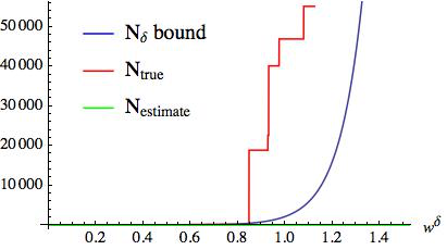
Figure 4 illustrates our results. Possible values of $w^{\delta}$ appear along the abscissa. The blue (gently sloping) curve shows the $N_{\delta}$ bound, calculated from forward-trial samples, in Theorem 1. The red (staggered) curve, calculated from reverse-trial samples, shows after how many reverse trials ($N_{\rm true}$) $W\geq w^{\delta}$ was extracted during one trial. $N_{\rm true}$ has a jagged, step-like shape, as one might expect.

The green curve (flat) lies close to the abscissa. This curve depicts the estimate, in [13], of the number of reverse trials expected to be performed before one trial outputs a dominant work value, for an unspecified meaning of “dominant.” We calculated $N_{\rm est}=3$ by simulating forward trials, calculating the average dissipated work, and substituting into Relation (6).

The curves’ shapes and locations illustrate the $N_{\delta}$ bound’s advantages. The bound (the blue, gently sloping curve) hugs the actual number $N_{\rm true}$ of trials required (the red, staggered curve) more closely than $N_{\rm est}$ (the green, flat curve) does. $N_{\rm est}$ remains flat, whereas the $N_{\delta}$ bound rises as $N_{\rm true}$ rises. The $N_{\delta}$ bound often lower-bounds $N_{\rm true}$, as expected. When $w^{\delta}$ is small, the $N_{\delta}$ bound weaves above and below $N_{\rm true}$, as shown in Fig. 5. The reason was explained above Theorem 1: $N_{\delta}$ denotes the number of trials expected, in a sense defined by probability and frequency, to be required. One might get lucky and extract $W\geq w^{\delta}$ before performing $N_{\delta}$ trials. The dropping of the $N_{\rm true}$ curve below the $N_{\delta}$ bound represents such luck. But one expects to perform $N_{\delta}$ trials, and the $N_{\delta}$ bound lower-bounds $N_{\rm true}$ for most $w^{\delta}$-values.

Conclusions—We have sharpened predictions about the number of experimental trials required to estimate $\Delta F$ from fluctuation relations. We improved the approximation in [13] to an inequality, tightened the bound (in scenarios of interest) with an entropy $H^{\beta}_{\infty}$, freed the experimenter to choose a tolerance $w^{\delta}$ for dominance, and approximately bounded the error in an estimate of $\Delta F$. How to choose $w^{\delta}$ merits further investigation. We wish to be able to specify the greatest error $\epsilon$ acceptable in an estimate of $\Delta F$. From $\epsilon$, we wish to infer the number $N^{\epsilon}$ of trials we should expect to perform. This entire investigation improves the rigor with which free-energy differences $\Delta F$ can be estimated from experimental and numerical-simulation data.

Acknowledgements—NYH thanks Yi-Kai Liu for conversations about error probability and thanks Alexey Gorshkov for hospitality at QuICS. Part of this research was conducted while NYH was visiting the QuICS and the UMD Department of Chemistry and Biochemistry. NYH was supported by an IQIM Fellowship and NSF grant PHY-0803371. The Institute for Quantum Information and Matter (IQIM) is an NSF Physics Frontiers Center supported by the Gordon and Betty Moore Foundation. CJ was supported by NSF grant DMR-1506969.

References

- [1] A. Pohorille, C. Jarzynski, and C. Chipot, J. Phys. Chem. B 114, 10235 (2010), http://dx.doi.org/10.1021/jp102971x, PMID: 20701361.
- [2] C. M. Rohwer, F. Angeletti, and H. Touchette, ArXiv e-prints (2014), 1409.8531.
- [3] N. Lu and D. A. Kofke, J. Chem. Phys. 114, 7303 (2001).
- [4] N. Lu and D. A. Kofke, J. Chem. Phys. 115, 6866 (2001).
- [5] J. Gore, F. Ritort, and C. Bustamante, 100, 12564 (2003).
- [6] D. Wu and D. A. Kofke, J. Chem. Phys. 121, 8742 (2004).
- [7] D. Wu and D. A. Kofke, Phys. Rev. E 70, 066702 (2004).
- [8] D. Wu and D. A. Kofke, J. Chem. Phys. 123, 054103 (2005).
- [9] D. Wu and D. A. Kofke, J. Chem. Phys. 123, 084109 (2005).
- [10] D. A. Kofke, Molecular Physics 104, 3701 (2006).
- [11] A. M. Hahn and H. Then, Phys. Rev. E 80, 031111 (2009).
- [12] S. Kim, Y. W. Kim, P. Talkner, and J. Yi, Phys. Rev. E 86, 041130 (2012).
- [13] C. Jarzynski, Phys. Rev. E 73, 046105 (2006).
- [14] N. Yunger Halpern, A. J. P. Garner, O. C. O. Dahlsten, and V. Vedral, New Journal of Physics 17, 095003 (2015), 1409.3878.
- [15] G. E. Crooks and C. Jarzynski, Phys. Rev. E 75, 021116 (2007).
- [16] M. Campisi, P. Hänggi, and P. Talkner, Rev. Mod. Phys. 83, 771 (2011).
- [17] G. E. Crooks, Physical Review E 60, 2721 (1999).
- [18] C. Jarzynski, Physical Review Letters 78, 2690 (1997).
- [19] T. M. Cover and J. A. Thomas, Elements of Information Theory (John Wiley & Sons, 2012).
- [20] R. Renner and S. Wolf, Smooth Rényi entropy and applications, in International Symposium on Information Theory, 2004. ISIT 2004. Proceedings., pp. 232–232, IEEE, 2004.
- [21] D. Collin et al., Nature 437, 231 (2005).
- [22] H. T. Quan and H. Dong, arXiv e-print (2008), 0812.4955.
- [23] H. Tasaki, eprint arXiv:cond-mat/0009244 (2000), cond-mat/0009244.
- [24] J. Kurchan, eprint arXiv:cond-mat/0007360 (2000), cond-mat/0007360.