Weakly bound states in heterogeneous waveguides: a calculation to fourth order

It is nowadays a well–known fact that bound states can appear in infinite waveguides or tubes, in presence of an arbitrarily weak bending or of a local, small, enlargement of its section. This behavior has been proved for general configurations in Refs. [1, 2] and it has been investigated for several specific geometrical configurations. It is impossible to refer to all the different works, but we would like to mention the case of the infinite symmetric cross studied by Schult and collaborators in Ref. [3]. Although Ref. [3] is focussed on the study of the quantum mechanical bound states of the symmetric cross, the problem is relevant in many areas of Physics, such as Acoustics, Electromagnetism and Fluid dynamics (in this respect, it is important to cite the work by Ursell Ref.[5, 6] who studied the emergence of trapped modes in a semi-infinite canal of fixed width terminating in a sloping beach). It is also important to mention that the appearance of bound states in waveguides and, more in general, in open geometries, must affect the transport properties of the systems, modifying the transmission and reflection coefficients (see for instance Ref. [4]).

From a mathematical point of view, one needs to solve the Helmholtz equation on an open, infinite domain, with Dirichlet boundary conditions at the border. In particular, Bulla and collaborators have considered in Ref. [7] the problem of an infinite homogeneous waveguide on the region

obeying Dirichlet boundary conditions at the border, assuming that $f$ is a $C^{\infty}({\mathbb{R}})$ function of compact support with $f\geq 0$. In their calculation $\lambda>0$ is a parameter which controls the deformation of the border (particularly the case $\lambda=0$ reduces to a straight waveguide, with a purely continuum spectrum). These authors were able to show that, if $\int_{-\infty}^{\infty}f(x)dx>0$, there is at least one eigenvalue falling below the continuum threshold. They also obtained the exact expression for the energy of the fundamental mode, to second order in the parameter controlling the deformation. Soon after, Exner and Vugalter [8] studied this problem, when the deformation of the border averages out, i.e. when $\int_{-\infty}^{\infty}f(x)dx=0$. Interestingly they found out that under certain conditions it is still possible to have a bound state and that the energy gap scales as the fourth power in $\lambda$.

Recently, the present author and collaborators have studied in Ref. [9] a different but related problem: the case of a infinite straight waveguide containing a small inhomogeneity centered at an internal point (assuming Dirichlet boundary conditions at the border). In that case, it was proved that, when the heterogeneity corresponds to a locally denser region, the eigenfunction of the ground state becomes localized around the heterogeneity and the corresponding energy falls below the continuum threshold. The calculation of Ref. [9] was carried out using perturbation theory up to third order, using an approach originally proposed by Gat and Rosenstein in Ref. [10] for a different problem. As a matter of fact, the implementation of the perturbative scheme must be done with care, since the naive identification of the unperturbed operator with the negative Laplacian would lead to the appearance of divergent contributions in the coefficients of the perturbative series for the energy of the ground state. The emergence of these (infrared) divergences can be easily understood since the spectrum of $(-\Delta)$ on an infinite strip is continuous and therefore the denominators of the coefficients in the Rayleigh-Schrödinger expansion may become arbitrarily small. To avoid this problem in Ref. [9] a suitable unperturbed operator was used, following the approach of Gat and Rosenstein: the spectrum of this operator contains now a localized state and the continuum, with the energy of the localized state falling below the continuum threshold (the separation between the two depends on a parameter $\beta$ in the unperturbed operator which will be eventually set to zero). In this way one is able to carry out the usual perturbative expansion, obtaining explicit expressions which are finite when $\beta\rightarrow 0^{+}$.

In this paper we have extended the calculation of Ref. [9], obtaining the exact general expression for the energy correction to fourth order in the density perturbation. The greater technical difficulty of the present calculation derives both because from the larger number of terms and both from their different nature. Working in our perturbation scheme we find that all the infrared divergent terms (i.e. terms which diverge as $\beta\rightarrow 0^{+}$) potentially contained in $E_{0}^{(4)}$ correctly cancel out, as expected. Moreover, for the case where the second and third order corrections both vanish, we find that there is a non–vanishing fourth order correction to the energy of the fundamental mode, which lowers the energy below the continuum threshold. Since the problem of Bulla et al. [7] may be converted to the problem of an infinite heterogeneous waveguide, using a suitable conformal map, our results also provide an alternative approach to the problems studied in Refs.[7] and [8]. Additionally, our formulas apply as well to the case of infinite heterogeneous and deformed waveguides (in this case the ”density” in our formulas would involve both the physical density of the waveguide and the ”conformal density” obtained from the mapping), thus allowing to treat more general problems.

The paper is organized as follows: in Section 2 we discuss the perturbation theory, and present the general formulas for the energy to fourth order; in Section 3 we consider a solvable model, reproducing the exact results to fourth order; in Section 4 we present our conclusions. The Appendices A and B contain technical details of the calculation.

In a recent paper we have obtained the explicit expression for the energy of the fundamental mode of an infinite, weakly heterogeneous two dimensional waveguide, up to third order in the density perturbation. It is assumed that the inhomogeneity is small and localized at some internal point of the waveguide. Under these assumptions it is proved that, when the perturbation corresponds to a locally denser material, a bound state, localized at the inhomogeneity appears.

Mathematically, we are considering the Helmholtz equation

where $|x|<\infty$ and $|y|\leq b/2$. The solutions obey Dirichlet boundary conditions at the border

and $\Sigma(x,y)>0$ for $|x|<\infty$ and $|y|\leq b/2$.

Expressing the density as $\Sigma\left(\mathbf{x}\right)=1+\sigma\left(\mathbf{x}\right)$, where $\lim_{|x|\rightarrow\infty}\sigma\left(\mathbf{x}\right)=0$, and assuming that $|\sigma(x)|\ll 1$ for $x\in(-\infty,\infty)$, we can perform a perturbative expansion in the density perturbation.

The general formulas for the perturbative corrections to the energy of the fundamental mode up to third order have been derived in Refs. [9] and [11] and read

where

and $\epsilon_{n}$ and $|n\rangle$ are the eigenvalues and eigenstates of the unperturbed operator¹¹ 1 In the following we will adopt the notation $\langle\hat{A}\rangle$ to indicate the expectation value of the operator $\hat{A}$ in the ground state of $\hat{H}_{0}$..

As we have discussed in Ref. [9], the identification of the unperturbed operator must be done with care, for the case of an infinite waveguide: as a matter of fact, the obvious candidate, corresponding to an infinite, straight and homogeneous waveguide cannot be used, since its spectrum is continuous and the fundamental mode can thus be excited to states which are arbitrarily close in energy. In this case, the perturbative formulas would contain infrared divergences, which would completely spoil the calculation. In a different context Gat and Rosenstein [10] have devised a perturbation scheme that allows to avoid these infrared divergences: in our case this process amounts to use as unperturbed operator

where $\beta$ is an infinitesimal parameter to be set to $0$ at the end of the calculation.

As discussed in Ref. [9], the basis set of eigenfunctions of $\hat{H}_{0}$ is

where

and

The eigenvalues of $\hat{H}_{0}$ are ²² 2 Notice that $\epsilon_{0,1}=-\beta^{2}+\frac{\pi^{2}}{b^{2}}<\frac{\pi^{2}}{b^{2}}$ and therefore it is separated from the continuum.

We find convenient to introduce the Dirac notation $|0,n\rangle$, $|p^{(e)},n\rangle$ and $|p^{(o)},n\rangle$ to indicate the eigenstates of $\hat{H}_{0}$.

Using the explicit form of the eigenfunctions of $\hat{H}_{0}$ given above, one can work out the perturbative expressions for the energy and, after taking the limit $\beta\rightarrow 0^{+}$, obtain the finite expressions given in Ref. [9]:

where ³³ 3 Notice that we have changed the notation of Ref. [9] to allow referring to more general Green’s functions.

Before discussing the fourth order, it is worth to comment that, as discussed in [9], a bound state is present only if the condition

is met.

We briefly review the discussion in Ref. [9]: the condition (13) can be derived calculating the Rayleigh quotient

using the variational function

and minimizing with respect to the variational parameter $a$:

Given that, in order to obtain a bound state, $a$ must be positive, the condition (13) follows.

In a similar way, one can derive the expression for the perturbative correction to the energy of the fundamental mode to fourth order; we find

The perturbative expressions written above must be evaluated taking the limit $\beta\rightarrow 0^{+}$ at the end of the calculation. For this reason it is convenient to work on the expectation values which appear in the expression and expand them around $\beta=0$.

For example, in the simplest case we have

The expressions for the remaining expectation values can be found in Appendix B. In particular, in Table 1 the coefficients $\kappa_{n}^{(j)}$ are subdivided into two classes: those which only contain longitudinal contributions (left column) and those which contain both longitudinal and tranverse contributions (right column).

Upon substitution of these expressions in the perturbative contributions of the energy we have

and

where

Observe that the potentially divergent terms in $E_{0}^{(3)}$ and $E_{0}^{(4)}$ only depend on the contributions stemming from the longitudinal excitations. While it was already proved in Ref. [9] that $E_{0}^{(3)}$ is finite for $\beta\rightarrow 0^{+}$, as it can be checked explicitly using the results in B, it is straightforward to verify that $\eta_{4a}=\eta_{4b}=0$. Therefore $E_{0}^{(4)}$ is finite for $\beta\rightarrow 0^{+}$, as expected.

Using the expressions in the Appendix we have

and

where $\eta_{4d}^{\parallel}$ contains only contributions from longitudinal modes while $\eta_{4d}^{\perp}$ contains contributions also from trasversal modes.

Their explicit expressions are ⁴⁴ 4 The expression for $g_{2}^{(0,0)}(x_{1},y_{1},x_{2},y_{2})$ is reported in A.

We may write the perturbative formulas obtained above in a more compact form as

where we have introduced the definitions

where $\Delta_{1}$ is the total extra mass of the inhomogeneous waveguide.

The energy up to fourth order can then be arranged in the form

where

When we apply the formulas above to the solvable model discussed in Ref. [9] we obtain

which reproduces the exact expression for the fourth order contribution reported in Ref. [9].

The case where the second and third order contributions vanish is particularly interesting and it deserves a detailed discussion. This situation is analogous to the case discussed by Exner and Vugalter in Ref. [8] for a uniform, weakly deformed, waveguide.

As previously observed in Ref. [9] this occurs when the density obeys the property

In this limit the general formulas obtained in the previous section reduce to

and the energy of the fundamental mode falls below the threshold of the continuum, signalling that the corresponding eigenfunction is localized in the region of the heterogeneity.

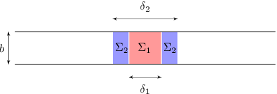
To test this prediction, we consider a solvable model, represented by an infinite heterogeneous waveguide, parallel to the horizontal axis and obeying Dirichlet boundary conditions on $y=\pm b/2$ (see Fig. 1).

The density is

where $\delta_{2}\geq\delta_{1}\geq 0$ (for $\sigma_{1}=\sigma_{2}$ this problem reduces to the one discussed in Ref. [9]).

We look for the solution to the Helmholtz equation

in the form

References

• [1] P. Exner, P. Seba, J. Math. Phys. 30, 2574 (1989)
• [2] J. Goldstone, R. L. Jaffe, Phys. Rev. B 45, 14100 (1992)
• [3] R. L. Schult, D. G. Ravenhall, H.W. Wyld, Phys. Rev. B 39, 5476 (1989)
• [4] S. Qu and M. R. Geller, Phys. Rev. B 70, 085414 (2004)
• [5] F. Ursell, Proc. Camb. Phil. Soc. 47, 348 (1951)
• [6] F. Ursell, Proc. R. Soc. Lond. A 214, 79 (1952)
• [7] W. Bulla et al., Proc. Amer. Math. Soc. 125, 1487 (1997)
• [8] P. Exner, S. A. Vugalter, Lett. Math. Phys. 39, 59 (1997)
• [9] P. Amore, F.M.Fernández and C.P. Hofmann, European Physical Journal B 89, 163 (2016)
• [10] G. Gat, B. Rosenstein, Phys. Rev. Lett. 70, 5 (1993)
• [11] P. Amore, J. Math. Phys. 51, 052105 (2010)
• [12] Till Tantau, “The TikZ and PGF Packages”, Manual for version 3.0.0, http://sourceforge.net/projects/pgf/, 2013-12-20.