Control of an Aerial Manipulator using On-line Parameter Estimator for an Unknown Payload
Abstract
This paper presents an estimation and control algorithm for an aerial manipulator using a hexacopter with a 2-DOF robotic arm. The unknown parameters of a payload are estimated by an on-line estimator based on parametrization of the aerial manipulator dynamics. With the estimated mass information and the augmented passivity-based controller, the aerial manipulator can fly with the unknown object. Simulation for an aerial manipulator is performed to compare estimation performance between the proposed control algorithm and conventional adaptive sliding mode controller. Experimental results show a successful flight of a custom-made aerial manipulator while the unknown parameters related to an additional payload were estimated satisfactorily.
I Introduction
Mobile manipulation is a key to many applications of robotics such as construction sites, production lines and space environments. Among them, aerial manipulation is receiving attention for aerial transportation or inspection of hard-to-reach structures due to the superior mobility in three dimensional Euclidean space [1].
Aerial manipulation can be divided into two categories based on the connection mechanism to a payload. The first approaches suspend a payload via a cable [2]. In [2], they developed a control logic for equilibrium of the payload at a specific desired pose using three aerial manipulators. However, the possible pose of a payload is limited. The second approaches are to grasp and move the object by using a robotic arm [3, 4, 5, 6]. In [3], a dynamic model was derived by the Euler-Lagrangian formulation and cartesian impedance controller was designed for aerial manipulators. A tracking control law for the end effector was designed and tested in simulation based on decoupled Lagrangian dynamics [4]. In [5], an aerial manipulator was developed for remote safety inspection of industrial plants. In [6], they custom-made an aerial manipulator with a 2-DOF robotic arm and designed integral backstepping controller. However, these papers do not consider the effect of unknown payload.
Handling of uncertain objects has been previously investigated for stationary manipulators or ground robots. [7, 8, 9, 10]. In [7, 8], they presented an adaptive controller for a ground robotic manipulator to handle an unknown object. Control of a constrained ground manipulator with parameter uncertainty was shown in [9]. They designed an adaptive controller for trajectory and force tracking problems. The mass and inertia properties of a simple mobile robot are estimated by an adaptive estimator in [10].
Research for aerial manipulators to handle an unknown object is still rare [11, 12, 13]. In [11], an adaptive sliding mode controller for an aerial manipulator was designed for coping with the parametric uncertainties. They demonstrated picking up and delivering an object with custom-made aerial manipulator. However, there was no estimation results and analysis of safe operation points for an unknown object. In [12], they proposed trajectory optimization and control for a quadrotor with the suspended payload. For handling a load, they used conventional adaptive control as same with [7], but this method is weak to noise or disturbances because the adaptation rule only based on control error. In [13], they designed an estimator of external generalized forces acting on aerial robots. This algorithm is applicable for aerial manipulator, but the performance for moving an unknown object has not been demonstrated by experiments.
There are researches on control of mechanical manipulators or aerial vehicles including estimation of unknown mass [14, 15]. In [14], they estimated the physical properties of a mechanical manipulator using least-squares method based on sensing of joint torque. However, this conventional estimation approach cannot be applied to small aerial manipulators, because the payload limitation does not allow to equip the heavy torque sensors.In [15], they developed a quadrotor with a gripper and used batch least-square method for estimating unknown mass using control input and acceleration data only. The estimation algorithm therein was designed for a quadrotor in hover or near-hover condition, but the dynamics will become more complicated for an aerial manipulator with a robotic arm.

The contributions of this paper can be summarized as follows: First, we design an on-line parameter estimator for the aerial manipulator. The unknown properties of a payload are estimated by the parameter estimator based on parametrization of the combined system, which considers a hexcopter and a robotic arm as a unified system. Unlike [15], the estimator does not depend on the flight condition. Second, an augmented passivity-based controller is designed to stabilize the aerial manipulator with the estimated parameters. Third, we apply this control algorithm to our custom-made aerial manipulator as shown in Fig. 1 and show feasibility of the proposed control algorithm for the aerial manipulator in the simulation and experiment.
This paper is structured as follows: in section II, we describe the dynamics of an aerial manipulator. The parameter estimator and controller are designed in section III. Section V presents results from experiments in which the aerial manipulator estimates the unknown parameters of a payload on the flight. Section VI contains concluding remarks.
II Dynamics of Aerial Manipulator
This section presents the dynamics of aerial manipulator. The more detailed kinematic relations and equations of motion can be found in our previous research [11].

II-A Dynamics for the Combined System
Fig. 2 shows coordinated frames for the dynamic model of an aerial manipulator. represent the inertial frame, the bodyframe of the hexacopter and the bodyframe of link , respectively. The subscript denotes the link number. Using the position of center of mass of the hexacopter in the inertial frame , Euler angles of the hexacopter and joint angles of the manipulator , the dynamic model can be described based on the following system state,
The equations of motion of the combined system with the state can be derived as
| (2) |
where is the control input, is the inertia matrix, is the Coriolis matrix, and is the gravity term. Here, two elements of , i.e. and , are used to generate the desired roll and pitch angle . They are computed by the following rule:
This relation is derived based on the small roll and pitch angle assumption.
II-B System Parametrization

When the end effector grasps a single object, the physical properties of link 2 change. Total mass of second link, is changed by additional payload and initial mass of second link , i.e. as shown in Fig. 3. Also, if the additional payload is treated as a point mass, then the change of moment of inertia is easily computed by the parallel axis theorem [16]:
| (9) |
where is the changed moment of inertia with respect to rotational axis of second link and is length of second link.
Since and other physical information about hexacopter and link 1 are already known values, therefore, the equation of motion is parameterized with respect to the unknown mass and the length of center of mass at link 2, . Here, is the total mass of link 2 including the unknown payload. In this case, we can separate , and into the matrices with known parameters and unknown parameters:
| (10) |
Here , and are the matrices with known physical parameters and the others are the matrices with unknown parameters, such as unknown mass and , . Using these matrices (10), the dynamic equations (2) can be written as the following parameterized form:
| (11) |
III Estimator and Controller Design
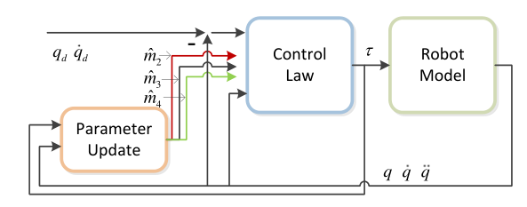
In this section, we design on-line parameter estimator and the augmented passivity-based controller for the hexacopter with the robotic arm. The total control structure is shown as Fig. 4.
III-A On-line Parameter Estimator for an Unknown Payload
In order to estimate the physical properties of an unknown payload, a parameter estimation law for an aerial manipulator is developed based on the parametrization of dynamic equation (12). For a parameter estimator, we assumed that , and are constant parameters to be identified on-line. We also assumed that , and are available with the forcing term which makes bounded. Note that the second assumption can be relaxed by the control law. Based on these assumptions, the state estimator equation appears as
| (14) |
where and are user-defined positive definite gain matrices. Here, , and . are the estimated parameters. Note that should be satisfied for estimation.
If we define the state error as
| (15) |
where is the estimated state. The parameter update rules can be given as
| (16) |
where, the positive numbers are the learning rate of parameter estimator.
Proposition: The error dynamics (17) is asymptotically stable.
Proof:
In order to prove the convergence of the estimation error dynamics (14), we define the following Lyapunov candidate function:
| (18) |
The time derivative of is given as:
Using the fact that , the parameter estimator rule (16) results in:
| (19) |
where denotes the smallest eigenvalue of the matrix . This proves the bounded of , , , . If is bounded, then is bounded by (17). Then, is also bounded, which guarantees that state estimation error, goes to 0 as time goes infinity by application of Barbalat’s lemma [17]. ∎
The proof of convergence when persistence of excitation is assumed, i.e., , follows from standard results in [14]. The detailed proof is omitted due to length limitation.
III-B Augmented Passivity-based Controller Design
In this subsection, we design the controller for the aerial manipulator. Applying the estimated parameters , and to the controller, a augmented passivity-based control law is designed with following state error as
| (20) |
Here, we assumed that the desired trajectory is bounded as follows:
| (21) |
where is a positive constant.
The augmented passivity-based control for robotic manipulators using the estimated parameters can be written as the following equation:
| (22) |
where and are diagonal gain matrices. , and represent the estimation of each matrix by parameter update rule (16), i.e. , and .
Before proving the stability, we define a regressor matrix, for simplicity and it appears as:
| (23) |
where , is the estimation of and
| (24) |
where , , and .
The closed-loop dynamics can be derived by substituting the proposed control law (22) into (2) and using (24):
| (25) |
With these equations, stability analysis can be performed as the following, which shows the boundedness of error and .
Proof:
We define the following Lyapunov candidate function:
| (26) |
The time derivative of can be expressed as:
| (27) | ||||
In the derivation, skew symmetricity of is used [18]. Although , the term is bounded by the parameter estimator. In this case, if we choose a gain sufficiently large, we can show that is ultimately bounded. However, if we have the parameter convergence under the proposed estimator in (14), i.e., , we can show that . In this situation, as same with (19), we can show asymptotic stability of the proposed controller by application of Barbalat’s lemma [17]. ∎
IV Simulation Results
Precise estimation of parameters is important for handling an unknown payload. Therefore, in this section, simulation for an aerial manipulator is performed to compare estimation performance between the proposed control algorithm and conventional adaptive sliding mode controller.
IV-A Mass Estimation using Adaptive Sliding Mode Controller
An adaptive sliding mode controller for an aerial manipulator is shown in [11]. For performance comparison with the proposed method, we also implemented a simple estimation algorithm described below, which is modified based on [15] for an additional payload.
To design an adaptive sliding mode controller, we can define the sliding surface and virtual reference trajectory as
| (28) | ||||
where is a diagonal gain matrix.
The adaptive sliding mode controller appears as
| (29) |
where and are the diagonal gain matrices and is the adaptation term for cancelling out the modelling error and disturbances. Also, , and are the function of the states, i.e., and the estimated unknown mass .
We can extract the unknown mass information of a payload using the adaptive sliding mode controller by the following equation:
| (30) | ||||
where the subscript is the third row of the matrix , are previously estimated mass and is total mass of the arial manipulator containing the unknown mass. Here and , which are already known, are the mass of a hexacopter or link 1, respectively.
IV-B Hexacopter with Robotic Arm Model
The parameters of a hexacopter with two-DOF robotic arm under consideration are given in Table. I. Properties of the Firefly hexacopter are from [19]. Here is the length of link . The mass of a payload is set to be , i.e., kg.
| Parameter | Value | Parameter | Value |
|---|---|---|---|
| 1.0 kg | 0.013 kgm2 | ||
| 0.013 kgm2 | 0.021 kgm2 | ||
| 0.1kg | 0.2m |
* : initial value.
IV-C Simulation Results
Parameter estimation was simulated in time interval with , , , , . Gains for the proposed control law are set as , .
For the estimation of unknown parameters, we set the initial estimated state as . We also set initial value of unknown parameters as , and . Additional payload is set to be kg, i.e. and .
The desired trajectory that the aerial manipulator should follow is set to be as
| (31) |
where and are specified by (II-A).
Fig. 5 shows the position tracking performance. The red dashed line is the desired trajectory and the blue solid line is the trajectory of the aerial manipulator using the proposed control algorithm. Fig. 6 shows the estimator performance and results of estimated parameters. The blue solid line is the state of the aerial manipulator and the red dashed line is the estimated state by the parameter estimator.
With the proposed control algorithm, the aerial manipulator satisfactorily tracks the desired trajectory even when there exists an unknown payload. The unknown parameters , and are estimated precisely as shown in Fig. 6b. However, when using the adaptive sliding mode controller (29) and (30), the performance of estimation became worse than the proposed control law as shown in Fig. 6b. This is mainly because the adaptive sliding mode control algorithm can estimate the unknown mass only while the parameter estimator estimate the whole unknown parameters, .


V Experimental Results
In this section, we describe experimental results with a custom-made aerial manipulator, which is composed of a hexacopter and a 2-DOF robotic arm.
For facilitating easier implementation, we use the following simplicity assumptions:
- •
Roll and pitch angles are small, i.e., and .
- •
At link 1, center of mass is located at joint angle, i.e. .
Using these two assumption, the on-line parameter equation (14) and the proposed controller (22) can be implemented much simpler.
V-A Experimental Setup
The hexacopter used in this paper is a Ascending Technlogies Firefly hexacopter [20]. The robotic arm is customized with Dynamixel servomotors. The total length of arm is 0.305 meter: meter and meter. The total weight of robotic arm is about 0.220 kg before picking up the payload.
The experimental setup is shown in Fig. 7. Vicon, an indoor GPS system, gives the position informations with 100 Hz to the base computer. The desired and current states of a hexacopter and the joint angles are transmitted to the hexaxcopter with Xbee at 40 Hz. The parameter estimator and augmented controller runs at 1 kHz in the onboard processor of Firefly hexacopter. Arm control inputs are sent by Bluetooh at 50 Hz.
V-B Experimental Results

The proposed control algorithm using a parameter estimator and controller is validated by an experiment. The flight result is shown in Fig. 8
Fig. 8a compares state tracking performance between the proposed controller and conventional non-adaptive controller. The conventional controller means that the controller does not have update rule for the unknown parameter in (22). The red dashed lines show the desired trajectory based on each controller, the blue solid lines represent states with the proposed approach and the black dash-dot lines are states with conventional approach. In Fig. 8a, the desired joint angles are fixed at degree and degree, respectively, (i.e. the arm is almost stretched to the side.) From the entire trajectory histories, although a large torque is applied due to this particular pose, the proposed controller shows satisfactory tracking results. On the other hand, the conventional approach cannot track the desired trajectory because this controller cannot compensate the effect of the unknown payload.
Fig. 8b shows estimator performance and parameter estimation results. The blue solid lines are real state of the aerial manipulator and the red dashed lines show the result by parameter estimator. The parameter estimator estimates current trajectory of the aerial manipulator satisfactorily. The parameter estimator shows good convergence to the true mass of at 0.238 kg (the additional payload is 0.120 kg for the extra payload and the gripper) and about 0.09 meter.
A video clip of the experiments is posted on the following URL: http://icsl.snu.ac.kr/hbeom/Estimation_AMS.mp4.
VI Conclusion
This paper presented a parameter estimation and control of an aerial manipulator for handling an additional payload. The unknown parameters of the payload were estimated and an augmented passivity-based controller was designed to control a hexacopter with a 2-DOF robotic arm. In the experimental results, we showed a successful flight using a custom-made aerial manipulator while the unknown parameters were estimated satisfactorily. Our future works include adaptive control of aerial manipulator for handling lumped uncertainty except the unknown payload.
References
- [1] R. D’Andrea, “Guest editorial can drones deliver?” IEEE Transactions on Automation Science and Engineering, vol. 11, no. 3, pp. 647–648, 2014.
- [2] N. Michael, J. Fink, and V. Kumar, “Cooperative manipulation and transportation with aerial robots,” Autonomous Robots, vol. 30, no. 1, pp. 73–86, 2011.
- [3] V. Lippiello and F. Ruggiero, “Exploiting redundancy in cartesian impedance control of uavs equipped with a robotic arm,” in IEEE/RSJ International Conference on Intelligent Robots and Systems (IROS), 2012, pp. 3768–3773.
- [4] H. Yang and D. Lee, “Dynamics and control of quadrotor with robotic manipulator,” in IEEE International Conference on Robotics and Automation (ICRA), 2014, pp. 5544–5549.
- [5] M. Fumagalli, R. Naldi, A. Macchelli, R. Carloni, S. Stramigioli, and L. Marconi, “Modeling and control of a flying robot for contact inspection,” in IEEE/RSJ International Conference on Intelligent Robots and Systems (IROS), 2012, pp. 3532–3537.
- [6] A. Jimenez-Cano, J. Martin, G. Heredia, A. Ollero, and R. Cano, “Control of an aerial robot with multi-link arm for assembly tasks,” in IEEE International Conference on Robotics and Automation (ICRA), 2013.
- [7] J.-J. E. Slotine and W. Li, “On the adaptive control of robot manipulators,” The International Journal of Robotics Research, vol. 6, no. 3, pp. 49–59, 1987.
- [8] Y.-C. Liu and M.-H. Khong, “Passivity-based teleoperation system for robots with parametric uncertainty and communication delay,” in IEEE International Conference on Automation Science and Engineering (CASE), 2014, pp. 271–276.
- [9] W. Dong, “On trajectory and force tracking control of constrained mobile manipulators with parameter uncertainty,” Automatica, vol. 38, no. 9, pp. 1475–1484, 2002.
- [10] S. S. Nestinger and M. A. Demetriou, “Adaptive collaborative estimation of multi-agent mobile robotic systems,” in IEEE International Conference on Robotics and Automation (ICRA), 2012, pp. 1856–1861.
- [11] S. Kim, S. Choi, and H. J. Kim, “Aerial manipulation using a quadrotor with a two dof robotic arm,” in IEEE/RSJ International Conference on Intelligent Robots and Systems (IROS), 2013, pp. 4990–4995.
- [12] I. Palunko, R. Fierro, and P. Cruz, “Trajectory generation for swing-free maneuvers of a quadrotor with suspended payload: A dynamic programming approach,” in IEEE International Conference on Robotics and Automation (ICRA), 2012, pp. 2691–2697.
- [13] F. Ruggiero, J. Cacace, H. Sadeghian, and V. Lippiello, “Impedance control of vtol uavs with a momentum-based external generalized forces estimator,” in IEEE International Conference on Robotics and Automation (ICRA). IEEE, 2014, pp. 2093–2099.
- [14] C. G. Atkeson, C. H. An, and J. M. Hollerbach, “Estimation of inertial parameters of manipulator loads and links,” The International Journal of Robotics Research, vol. 5, no. 3, pp. 101–119, 1986.
- [15] D. Mellinger, Q. Lindsey, M. Shomin, and V. Kumar, “Design, modeling, estimation and control for aerial grasping and manipulation,” in IEEE/RSJ International Conference on Intelligent Robots and Systems (IROS), 2011, pp. 2668–2673.
- [16] R. C. Hibbeler, Engineering mechanics. Pearson education, 2001.
- [17] H. K. Khalil and J. Grizzle, Nonlinear systems. Prentice hall Upper Saddle River, 2002, vol. 3.
- [18] R. M. Murray, Z. Li, and S. S. Sastry, A mathematical introduction to robotic manipulation. CRC press, 1994.
- [19] M. C. Achtelik, K.-M. Doth, D. Gurdan, and J. Stumpf, “Design of a multi rotor mav with regard to efficiency, dynamics and redundancy,” in AIAA Guidance, Navigation, and Control Conference, Minneapolis, MN, 2012.
- [20] “Ascending technologies, GmbH,” http://www.asctec.de.