Fermionic Hubbard model with Rashba or Dresselhaus spin-orbit coupling

It was well known that it is the strong electron correlations [1, 2, 3, 4, 5, 6] which lead to many important phenomena such as Anti-ferromagnetism, spin density wave, charge density wave, putative spin liquids with topological orders, un-conventional superconductivity,etc. The Rashba or Dresselhaus spin-orbit coupling (SOC) [7] is ubiquitous in various 2d or layered insulators, semi-conductor systems, metals and superconductors without inversion symmetry [8, 9, 12, 10, 11, 13, 14]. On the other forefront, due to their tunability and controllability, strongly correlated Fermi gases on optical lattices have been attempted with some success to quantum simulate some of these phenomena [15, 16]. There are very recent notable experimental advances in generating 2d Rashba or Dresselhaus SOC or any their linear combinations for cold atoms in both continuum and optical lattices [17, 18, 19, 20]. It becomes topical and important to investigate the combined effects of strong correlations and Rashba SOC in various lattice systems.

In this paper, we address this outstanding problem. Specifically, we investigate the system of interacting fermions at half filling hopping in a 2 dimensional square lattice subject to any combinations of Rashba or Dresselhaus SOC. In the strong coupling limit, we reach a novel quantum spin model named Rotated Anti-Ferromagnetic Heisenberg model (RAFHM) which is a new class of quantum spin models. For a special combination of the Rashba or Dresselhaus SOC, we identify a new spin-orbital entangled commensurate ground called Y-y state [21] subject to quantum fluctuations at $T=0$. We evaluate the quantum fluctuations by spin wave expansions up to $1/S^{2}$ order ( which is also called $1/S$ correction to the linear spin wave expansion ( LSWE ) in previous literatures on Heisenberg models ). It supports a massive relativistic commensurate magnon $C-C_{0}$ in one SOC parameter regime and an in-commensurate magnon C-IC in the other regime [21]. The two gap minima positions of the C-IC magnons are continuously tuned by the SOC strength. At low temperatures, these magnons dominate all the physical quantities such as the specific heat, magnetization, $(0,\pi)$ and $(\pi,0)$ susceptibilities, Wilson ratio and also various spin correlation functions. At $T=0$, the longitudinal spin structure factor shows a sharp peak at $\vec{k}=0$ in the reduced Brillouin Zone (RBZ) reflecting the ground state. However, the transverse spin structure factor displays non-trivial features reflecting the magnon excitations above the ground state. The $C-C_{0}$ leads to a pinned central Lorentzian peak at $\vec{k}=0$ in the TSSF. However, the $C-IC$ splits it into two Lorentzian peaks located at its two gap minima, while changing its structure at $\mathbf{k}=0$ into a saddle point one. In the weak coupling limit, any weak repulsive interaction leads to a weak Y-y state which also hosts low energy fermionic excitations. There is a crossover from the weak to the strong coupling where the fermionic excitation energies increase. The electronic and spin Wilson loops can be determined by measuring specific heats in high temperature expansion in weak and strong coupling limit respectively. The $C-IC$ encodes short-range incommensurate seeds embedded in an commensurate ground state at $T=0$, which justifies its name [21]. The crucial roles to be played by these seeds at generic SOC parameters $(\alpha,\beta)$ and under various external probes are outlined in the conclusion section. Experimental realizations and detections in both layered noncentrosymmetric materials and cold atom systems are discussed.

The tight-binding Hamiltonian of spin $1/2$ fermions at half filling hopping in a two-dimensional (2D) square optical lattice subject to any combination of Rashba and Dresselhaus SOC is:

where $t$ is the hopping amplitude along the nearest neighbors $\langle ij\rangle$, the non-Abelian gauge fields $U_{i\textsterling\textlnot i+\hat{x}}=e^{i\alpha\sigma_{x}}$, $U_{i\textsterling\textlnot i+\hat{y}}=e^{i\beta\sigma_{y}}$ are put on the two links in Fig.1a which is the lattice regularization of the linear combination $k_{x}\sigma_{x}+k_{y}\sigma_{y}$ of the Rashba and Dresselhaus SOC in a continuum momentum space [8, 11]. $\alpha=\pm\beta$ stands for the isotropic Rashba ( Dresselhaus ) case. $U>0$ is the Hubbard onsite interaction.

In the strong coupling limit $U/t\gg 1$, to the order $O(t^{2}/U)$, we obtain the effective spin $1/2$ Rotated anti-ferromagnetic Heisenberg model (RAFHM):

with the anti-ferromagnetic exchange interaction $J=4t^{2}/U>0$, $a,b=1,2,3$ are the three components of the spin operator, the $R(X,2\alpha)$, $R(Y,2\beta)$ are the two SO(3) rotation matrices around the $X$ and $Y$ spin axis by angle $2\alpha$, $2\beta$ putting on the two bonds along $\hat{x}$, $\hat{y}$ respectively.

Here, we plan to study the quantum or topological phenomena in the RH model at generic $(\alpha,\beta)$. However, it is a very difficult task, so we take a ”divide and conquer” strategy. First, we identify a solvable line $(\alpha=\pi/2,\beta)$ and explore new and rich quantum phenomena along the line. Then starting from the results achieved from the solvable line, then we will investigate the quantum phenomena at the generic $(\alpha,\beta)$ including the Rashba or Dresselhaus SOC point $\alpha=\pm\beta$. In this paper, we will focus on the first task. The second task will be outlined in the conclusion section and presented in details elsewhere. In the past, this kind of “divide and conquer” approach has been very successful in solving many quantum spin models. For example, in the single ( multi-) channel Kondo model, one solve the Thouless (Emery-Kivelson) line [22, 23], then do perturbation away from it. In quantum-dimer model, one solves the Rohksa-Kivelson (RK) point which shows spin liquid physics [24], then one can study the effects of various perturbations away from it [25]. Recently, this ”divide and conquer” strategy was quite successfully applied to study the RFHM along the solvable line first in [26], then at the generic SOC parameter in [27].

The RAFHM Eqn.2 inherits all the symmetries of the fermionic model Eqn.1. Along the line $(\alpha=\pi/2,\beta)$, in addition to own the spin-orbital coupled $U(1)_{soc}$ symmetry $[H_{f},\sum_{i}(-1)^{i_{x}}c_{i}^{\dagger}\sigma^{y}c_{i}]=0$, it also has an extra mirror ${\cal M}$ symmetry: under the local rotation $\tilde{\mathbf{S}}_{i}=R(\hat{x},\pi)R(\hat{y},\pi n_{2})\mathbf{S}_{i}$, then followed by a Time reversal transformation, $\beta\rightarrow\pi/2-\beta$. At the middle point $\beta=\pi/4$, the Hamiltonian is invariant under such a Mirror transformation. In the classical limit $S\to\infty$, one can show that the ground state is the $Y-y$ state in Fig.1a which still respects both the $U(1)_{soc}$ symmetry and the ${\cal M}$ symmetry which will be used to classify the symmetry of the minimum positions and the magnon gap in Fig.2. The $Y-y$ state also keeps the ${\cal P}_{y}$ and ${\cal T}{\cal P}_{x}$ and ${\cal T}{\cal P}_{z}$ symmetries.

Based on the $Y-y$ state in Fig.1a, we introduce the Holstein-Primakoff (HP) bosons $a$ and $b$ for the sublattice $A$ and $B$ respectively, the Hamiltonian Eq.(2) can be written in a systematic $1/S$ expansion in terms of the HP bosons [28, 29, 30, 31]:

where $\mathcal{H}_{0}=-2NJS^{2}$ is the classical ground state energy. The $\mathcal{H}_{2}$ represents linear spin wave theory, the $\mathcal{H}_{4}$ represents $1/S$ correction to linear spin wave theory [30] and so on. In the rest of the paper, we will use $2JS$ to be the energy unit.

By combining a unitary transformation, followed by a Bogoliubov transformation ( see the appendix A ), one can diagonize $\mathcal{H}_{2}$:

where the LSW spectrum $\omega_{k}^{\pm}=\sqrt{1-(\gamma_{k}^{\pm})^{2}}$ and $2\gamma_{k}^{\pm}=\cos 2\beta\cos k_{y}\pm\sqrt{\cos^{2}k_{x}+\sin^{2}2\beta\sin^{2}k_{y}}$. When $\beta<\pi/4$, $\omega^{+}_{k}<\omega^{-}_{k}$, when $\beta>\pi/4$, $\omega^{+}_{k}>\omega^{-}_{k}$, at $\beta=\pi/4$, $\omega^{+}_{k}=\omega^{-}_{k}$. So $\omega^{+}_{k}$ and $\omega^{-}_{k}$ are related by the ${\cal M}$ symmetry. In the following, for the notational simplicity, we call the lower branch $\omega^{-}_{k}$, the energy is measured in the unit of $4JS$.

Along the line $(\alpha=\pi/2,0<\beta<\pi/2)$, the position of the minima of the lower branch $\omega_{k}^{-}$ is given in Eq.A and shown in Fig.2a. One can see that when $0<\beta<\beta_{1}$ and $\beta_{2}=\pi/2-\beta_{1}<\beta<\pi/2$, the $Y-y$ ground state supports the C-C₀, when $\beta_{1}<\beta<\beta_{2}$, it supports the C-IC magnons. The low energy excitation can be obtained from the expansion around the minima $\mathbf{k}=\mathbf{k}_{0}+\mathbf{q}$ as:

where the mass $\Delta$ at the minima and the two velocities are given in Eqn.27 and shown in Fig.2b.

Thus, they are relativistic gapped particles with a gap $\Delta$ and two velocities $v_{x}\geq v_{y}$ where the equality holds at $\beta=0,\pi/4,\pi/2$. Near $\beta_{i},i=1,2$, $v_{y}\sim|\beta-\beta_{i}|^{1/2}$. In a sharp contrast, the C-IC magnons in the RFHM [26] are non-relativistic gapped particles with a gap $\Delta$ and two effective masses $m_{y}\geq m_{x}$.

At the two Abelian points $\beta=0,\pi/2$, the system has SU(2) symmetry in the rotated basis $\tilde{SU}(2)$ with $\tilde{\mathbf{S}}_{i}=R(\hat{x},\pi n_{1})\mathbf{S}_{i}$ and $\tilde{\tilde{SU}}(2)$ with $\tilde{\tilde{\mathbf{S}}}_{i}=R(\hat{x},\pi n_{1})R(\hat{y},\pi n_{2})\mathbf{S}_{i}$ respectively ( Fig.8 ), Eq.4 reduces to the AFM spin wave $\omega_{k}\sim k$ at the minimum $(0,0)$ and $(\pi,0)$ respectively.

We also obtain the ground-state energy and the magnetization at $T=0$ from the LSW:

which are drawn in Fig.3.

At low temperatures, one can drop the higher energy mode of the $\omega^{+}_{k}$ and evaluate the specific heat and the Staggered magnetization of the $Y-y$ state in Fig.4 due to the relativistic magnons:

where $M$ is the zero temperature staggered magnetization listed in Eq.6.

By coupling to the conserved quantity $-H_{s}\sum_{i}(-1)^{i_{x}}S_{i}^{y}$ and to the order parameter $-H_{s}\sum_{i}(-1)^{i_{y}}S_{i}^{y}$ respectively, one can also evaluate the $(\pi,0)$ and $(0,\pi)$ staggered susceptibilities:

where $\chi_{(0,\pi)}(T=0)=\sum_{k,s=\pm}\frac{1-(\omega_{k}^{s})^{2}}{2(\omega_{k}^{s})^{3}}$ is the zero temperature $(0,\pi)$ staggered susceptibility.

From the specific heat $C_{m}(T)$ in Eq.7 and the conserved $(\pi,0)$ staggered susceptibility $\chi_{(\pi,0)}(T)$ in Eq.8, one can form the Wilson ratio:

which only depends on [32] the dimensionless quantity of $T/\Delta(\beta)$.

The physical quantities in Eq.7 and 8 depend on explicitly the magnon’s two velocities $v_{x},v_{y}$ and its gap $\Delta$ shown in Fig.2b. However, the Wilson ratio in Eq.9 only depends on the gap $\Delta$. It is easy to see that the longitudinal spin structure factor always has a very sharp peak $M^{2}\delta_{\vec{k},0}$ at the ordering wavevector $(0,\pi)$ ( which is at $(0,0)$ in the RBZ ) of the Y-y state in Fig.1a with the spectral weight equal to the square of the magnetization. Unfortunately, the positions of the gap minima at $(0,k^{0}_{y})$ of the C-IC magnons in Fig.2a can not be reflected in all these physical quantities. In the following, we show that they can be precisely mapped out by the peak positions in the transverse structure factors.

Performing a local gauge transformation $\tilde{c}_{i}=(i\sigma_{x})^{i_{x}}c_{i}$ on Eqn.1, one can get rid of the gauge fields on all the $x-$ links, all the remaining gauge fields on the $y-$ links commute. Similarly, by performing a local rotation $\tilde{\mathbf{S}}_{n}=R(\hat{x},\pi n_{1})\mathbf{S}_{n}$ in Eqn.2, one can get rid of the $R$-matrix on the $x$-links shown in Fig.1b1. It makes the $U(1)_{soc}$ symmetry with the conserved quantity $Q_{c}=\sum\tilde{S}_{i}^{y}$ explicit, but at the expense of reaching the translational symmetry broken Hamiltonian with the $(\pi,0)$ sublattice structure in Fig.1b1. The $Y-y$ ground state in the original basis in Fig.1a becomes the $Y-(\pi,\pi)$ Neel state in the $U(1)$ basis in Fig.1b2. Because of the in-compatibility of the two sublattice structures in Fig.1b, one need to introduce four HP bosons $a,b,c,d$ corresponding to the 4-sublattice structure $A,B,C,D$ shown in Fig.1b2 respectively to perform the SWE.

Several physical quantities such as the magnitude of the magnetization $M_{Q}(T)$, specific heat $C_{m}$, the gaps $\Delta$ and density of state (DOS) are gauge invariant, so are the same in both basis. The $(\pi,0)$ and $(0,\pi)$ susceptibilities become the uniform and the $(\pi,\pi)$ staggered susceptibilities respectively in the $U(1)$ basis. The Wilson ratio is also gauge invariant after using the uniform susceptibility in the $U(1)$ basis. However, the spin-spin correlations functions are gauge dependent [33]. As shown in this section, it is the spin-spin correlations in the $U(1)$ basis which can map out the $C-C_{0}$ and $C-IC$ relativistic magnons most efficiently [26]. Due to the explicit $U(1)$ symmetries in the $U(1)$ basis, the anomalous structure factors $S^{++}=S^{--}=0$, so one need only evaluate the normal structure factors $S^{+-}$. However, due to the 4-sublattice structure in Fig.1b2, one need to evaluate it at 4 different orbital orders at $Q_{u}=(0,0),Q_{x}=(\pi,0),Q_{y}=(0,\pi),Q_{s}=(\pi,\pi)$. Due to the exact relations among them in the Reduced Brillioun Zone (RBZ):

one can combine them into a single structure factor in the EBZ: $0<k_{x},k_{y}<2\pi$

where the denominator is precisely the relativistic magnons spectrum $\omega_{k}^{s}$ listed below Eqn.4, the numerator contains $\gamma_{k}^{s}$ listed below Eqn.4 and the $\sin\theta_{k}$ is given in the unitary transformation Eqn.A2 in the appendix A.

The transverse structure factor Eqn.11 at several typical $\beta$ is shown in Fig.5 and its fine structure near $\beta=\pi/4$ is shown in Fig.6. When $0<\beta<\beta_{1}$ or $\beta_{2}<\beta<\pi/2$, the $C-C_{0}$ leads to a central peak at $\mathbf{k}=(\pi,\pi)$. At the Abelian point $\beta=0$ in Fig.5a, $S^{+-}(q)\sim\frac{\sqrt{2}}{q}$ where $k=(\pi,\pi)+q$. Obviously, the singularity at $(\pi,\pi)$ is due to the infra-red divergence of the Goldstone mode $\omega=ck$ in Eqn.11. At a small $\beta$ in the $C-C_{0}$ regime in Fig.5b:

where the $\Delta(\beta)\sim\sqrt{2}\beta$ is the gap opening due to the small $\beta$ listed in Eq.27 and shown in Fig.2b.

In Fig.5c, when $\beta_{1}<\beta<\beta_{2}$, the C-IC starts to splits the central peak into two peaks located around its two minima $\mathbf{k}=(\pi,\pi\pm k^{0}_{y})$ shown in Fig.2a, the $\mathbf{k}=(\pi,\pi)$ becomes a saddle point being maximum along the $k_{x}$ direction, minimum along the $k_{y}$ direction. In Fig.5d, at $\beta=\pi/4$, the two peaks are exactly located at the two minima $(\pi,\pi\pm\frac{\pi}{2})$ of the $C-IC$ shown in Fig.2a, each of the two well separated Lorentzian peaks is given by:

where $\Delta(\beta=\pi/4)=1/2$ is the largest gap at $\beta=\pi/4$ shown in Fig.2b. As shown in Fig.6, the two Lorentzian peaks are moving closer when $\beta<\pi/4$ or apart when $\beta>\pi/4$. So in the C-IC regime, the structure factor maps out precisely the dispersions of the C-IC relativistic magnons which are completely due to quantum fluctuations and intrinsically embedded in the quantum Y-y ground state at $T=0$.

It is constructive to contrast to RFHM where the sublattice structure of the transformed Hamiltonian $(\pi,0)$ is compatible with the classical FM state in the $U(1)$ basis [26], so one need only introduce two HP bosons to perform SWE. So one only need to form a uniform $S^{+-}_{u}(k)$ and a $(\pi,0)$ staggered transverse structure factor $S^{+-}_{s}(k)$ in the RBZ listed in Eqn.31 in [26]. One can also establish the exact relation $S^{+-}_{u}(k)=S^{+-}_{s}(k+(\pi,0))$, so one can combine them into a single structure factor in the EBZ. It is a Gaussian exponentially suppressed by $e^{-\Delta/T}$, peaked at $(0,\pm k^{0}_{y})$ with a temperature dependent width $\sigma_{x}=\sqrt{m_{x}(\beta)T}$ due to the thermal fluctuations at a finite $T$. This is because there is no quantum fluctuations at $T=0$. The $Y-x$ state is an exact eigenstate. The C-IC magnons do NOT exist at $T=0$, so they need to be thermally excited, so can only be detected at a finite $T$.

So far, we focused on the strong coupling expansion at $U\gg t$ where the RAFHM Eqn.2 holds and the charge degree of freedoms are frozen. It is also important to start from the weak coupling limit¡¡$U\ll t$ where one need to also consider charge fluctuations and study how it approaches the strong coupling limit. Using the identity $n_{i\uparrow}n_{i\downarrow}=\frac{1}{2}n_{i}-\frac{2}{3}\mathbf{S}_{i}^{2}$ to explicitly keep the spin SU(2) symmetry of the Hubbard interaction in Eqn.1, one can introduce a magnetic order parameter $\mathbf{M}_{i}$ to decouple the interaction term:

The evolution of the non-interacting Fermi surfaces (FS) along the line $(\alpha=\pi/2,\beta)$ is shown in Fig.7a. Due to the FS nesting conditions at the half-filling shown in Fig.7, any weak interaction will open gaps to the non-interacting FS when $\beta\neq\pi/2$. So one can perform a well controlled weak coupling analysis to determine the spin-orbit orders of the ground state and also the excitation spectra.

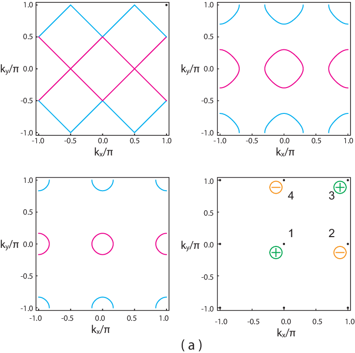
From the FS geometry in Fig.7a, there can only be four possible orbital orders $\mathbf{Q}_{1}=(0,0),\mathbf{Q}_{2}=(\pi,0),\mathbf{Q}_{3}=(0,\pi),\mathbf{Q}_{4}=(\pi,\pi)$. Substituting the order parameter $\mathbf{M}_{i}=\mathbf{M}e^{i\mathbf{Q}\cdot\mathbf{r}_{i}}$ where $\mathbf{Q}=\mathbf{Q}_{i},i=1,2,3,4$ and $\mathbf{M}=(X,Y,Z)$ into Eqn.14 leads to the mean field Hamiltonian: $H_{MF}=H_{0}+\frac{3N|\mathbf{M}|^{2}}{8U}$ and

where $T_{k}=-4t[\cos\beta\cos k_{y}\!-\!\sigma^{x}\sin k_{x}\!-\!\sigma^{y}\sin\beta\sin k_{y}]$ is the kinetic part of $H_{0}$ encoding the SOC parameters $(\alpha=\pi/2,\beta)$.

For $\mathbf{Q}_{3}=(0,\pi)$, diagonalizing the $4\times 4$ matrix in Eqn.15 leads to 4 fermionic energy levels $\pm\epsilon_{1},\pm\epsilon_{2}$. It is an insulating state with the P-H symmetry. Due to the lack of the spin $SU(2)$ symmetry, the minimization procedures are much more involved than those with the symmetry. We also take the ”divide and conquer ” strategy: first fixing the spin orientation and find the optimal magnitude and energy in the subspace, then determine the optimal orientation and magnitude. The results for the general spin orientation $\mathbf{M}=(X,Y,Z)$ is shown in Fig.7b. The global ground state has the $(0,Y,0)$ spin orientation, it is nothing but the $Y-y$ state which respects the $U(1)_{soc}$ symmetry. It also supports 2 branches gapped fermionic excitations listed in Eq.38. By repeating the calculations for $\mathbf{Q}_{4}=(\pi,\pi)$, we find the lowest spin-orientation is $X-(\pi,\pi)$ which breaks the $U(1)_{soc}$ symmetry. By applying the $U(1)_{soc}$ symmetry operator, one can see $X-(\pi,\pi)$ is degenerate with $Z-(0,\pi)$ which, of course, has higher energy than the $U(1)_{soc}$ symmetric $Y-y$ state as shown in Fig.7b.

For $\mathbf{Q}_{2}=(\pi,0)$ or $(0,0)$, it is the magnetic ordering in the P-P channel or hole-hole ( H-H ) channel, so breaks the P-H symmetry, both need a finite $U_{c}>0$ to reach a metallic state with only partial fillings of all the 4 fermionic bands $\epsilon_{i},i=1,2,3,4$. It has much higher energies than those insulating states in the P-H channel. So we conclude that the $Y-y$ states is indeed the global ground state at the weak coupling.

As shown in Fig.8, due to the $\tilde{SU}(2)$ and $\tilde{\tilde{SU}}(2)$ symmetry at the two Abelian points $\beta=0,\pi/2$ respectively, the Y-y state is degenerate with the other two states. However, away from them, the FS nesting conditions in Fig.7 at the half-filling favors the Y-y state which also supports the low energy fermionic excitations in Eq.38. So the specific heat in Eqn.7 will also receive the contributions from the fermionic part.

Following the procedures in [52], splitting the magnetic fluctuations into one longitudinal and two transverse components and performing Gaussian fluctuations above the $Y-y$ state, we can also identify the $C-C_{0}$ and $C-IC$ magnons from the poles of the dynamic transverse spin structure factor $S^{+-}(\vec{k},\omega)$. Of course, at the two Abelian points, the $C-C_{0}$ reduce to the two Gapless goldstone modes. They should smoothly crossover to those in Fig.2 achieved by the SWE in the strong coupling regime shown in Fig.7b. Note that the weak $Y-y$ state still respects the spin-orbital coupled $U(1)_{soc}$ symmetry $[H_{f},\sum_{i}(-1)^{i_{x}}c_{i}^{\dagger}\sigma^{y}c_{i}]=0$. However, the Mirror symmetry valid in the strong coupling limit does not hold anymore in the weak coupling limit. So there is a crossover from the weak to strong coupling where all the physical quantities evolve from having ${\cal M}$ asymmetry to owning ${\cal M}$ symmetry with respect to $\beta=\pi/4$. The next order terms $\sim t^{4}/U^{3}$ in the strong coupling expansion which include a ring exchange term around a fundamental square do not have such a Mirror symmetry. They may be needed to describe the crossover in Fig.8. The crossover driven by $U>0$ is dual to the BCS to BEC crossover driven by $U<0$ in SOC coupled Fermi systems discussed in [53].

In the classical fluctuation regime shown in the Fig.4, the $Y-y$ state to the paramagnet transition in the RAFHM is in the same universality class as that from $Y-x$ state to the paramagnet transition in the RFHM in [26] which was shown to be in the 2d Ising universality class [51]. In the high temperature regime in the Fig.4, from the high temperature expansions in the $T_{c}\sim J\ll T\ll U$ limit, one can easily establish the relation between the free energy of RAFHM and that of the RFHM in [26]:

Of course, the above relation breaks down in the symmetry breaking low temperature phases. Taking Eqn.18 in [26] and changing $J$ to $-J$ leads to high temperature expansion of the RAFHM:

where $W_{R}=2\cos 4\beta+1$ is the Wilson loop around the fundamental square given in the Sec.II. The discussions below Eqn.18 in [26] also apply here.

In the weak coupling $U\ll t\ll T$ limit, following the method in [8], we perform the high temperature expansion in the limit $T\gg t$ directly on the fermionic model Eq.1 to evaluate its specific heat:

which establishes its connection with the electronic Wilson loops $W_{f}$ given in Sec.I. Note that Eq.1 is invariant under $t\to-t$, so there is no odd power of $t/T$ term in the expansion, in contrast to Eqn.17 which has odd power of terms. The term in the $(t/T)^{4}$ power proportional to the electronic Wilson loop $W_{f}$ comes from the fermion hopping around a closed plaquette in the square lattice. Because $U\ll t$, so the interaction effects may be dropped in Eqn.18, so it is essentially a free fermions hopping in a non-abelain gauge potentials. So the crossover driven by the interaction $U$ at the low temperature $Y-y$ state in Fig.7 can also be partially seen by looking at the specific heat crossover from Eqn.18 to Eqn.17 in the high temperature paramagnet state.

In condensed matter systems, as said in the introduction, any of the linear superpositions of the Rashba SOC $k_{x}\sigma_{x}+k_{y}\sigma_{y}$ and Dresselhaus SOC $k_{x}\sigma_{x}-k_{y}\sigma_{y}$ always exists in various noncentrosymmetric 2d or layered materials. In momentum space, such a linear combination $\alpha k_{x}\sigma_{x}+\beta k_{y}\sigma_{y}$ can be written as the the kinetic term in Eq.1 in a periodic array of adsorbed ions with the SOC parameter $(\alpha,\beta)$ where the anisotropy can be adjusted by the strains, the shape of the surface or gate electric fields. The interaction strength $U$ in Eq.1 ranges from weak to strong in different materials [14, 13]. So all the phenomena in Fig.8 can be observed in these materials.

In the cold atom systems, in view of recent experimental advances to realize 2d Rashba or Dresselhaus SOC [17, 20], both the original and the $U(1)$ basis can be realized. Both gauge-invariant and non gauge-invariant quantities can be measured [33]. The gauge invariant quantities such as specific heat $C_{m}$ [37, 38], the gaps $\Delta$ and the DOS [39], the Wilson ratio can be detected by the corresponding experimental tools. The magnetization $M_{Q}(T)$, the $(\pi,0)$ and $(0,\pi)$ susceptibilities can be detected by the longitudinal atom or light Bragg spectroscopies [35, 36]. In the $U(1)$ basis in Fig.1b, one need to measure the transverse structure factor at the four different ordering wavevectors $Q_{u}=(0,0),Q_{x}=(\pi,0),Q_{y}=(0,\pi),Q_{s}=(\pi,\pi)$ in Eq.10 by the transverse atom or light Bragg spectroscopies [35, 36] to get the whole transverse structure Eqn.11 in the EBZ. Before reaching $T<T_{c}\sim J$, the specific heat measurement [37, 38] at high temperatures to determine the whole sets of fermionic or magnetic Wilson loops order by order in $t/T$ Eqn.18 or $J/T$ Eqn.17 could be performed easily. However, so far, the interaction in these cold atom experiments is still in weak coupling limit. So the weak Y-y state, both its fermionic and magnon excitations in Fig.8 can still be observed by various detection methods [34, 37, 38, 35, 36] in the current available weak coupling limit. Because there is only a crossover from the weak to the strong coupling, the results on magnons achieved in the strong coupling limit still hold qualitatively in the weak coupling limit. When the heating issue is completely overcame as the interaction strength is tuned to the strong coupling limit, the RAFHM Eqn.2 can be realized and all the strong coupling results achieved here can be detected quantitatively.

There are previous theoretical works to study strongly correlated spinless bosons in Abelian gauge fields [42, 43, 44, 45, 46] and spinor bosons in non-Abelian gauge fields [47, 48, 49, 26, 50, 51]. The topological quantum phase transitions of non-interacting fermions driven by a Rashba type of SOC are investigated in a honeycomb lattice [33]. Various itinerant phases and phase transitions of repulsively interacting fermions subject to Weyl type of SOC in a 3d continuum were studied in [52]. The BCS to BEC crossover of attractively interacting fermions tuned by the strengths of various forms of SOC in 2d and 3d continuum were explored in [53]. However, so far, there are very few works to study the possible dramatic effects of SOC on strongly correlated electron systems on lattice systems. In this paper, we investigate the system of interacting fermions at half filling hopping in a 2 dimensional square lattice subject to any combinations of Rashba and Dresselhaus SOC described by Eq.1. In the strong coupling limit, we reach a novel quantum spin model named Rotated Anti-Ferromagnetic Heisenberg model (RAFHM) Eq.2 which is a new class of quantum spin models. Along the anisotropic line $(\alpha=\pi/2,\beta)$, its ground state is a new kind of spin and bond correlated magnetic state called Y-y state in Fig.1a which supports a novel excitation called C-IC magnons in a large SOC parameter regime $\beta_{1}<\beta<\beta_{2}$ in Fig.2a.

The C-IC magnons in the RAFHM stand for the short-ranged IC seeds embedded in a commensurate long-range ordered Y-y state. Their parameters such as the minimum positions $(0,k^{0}_{y})$, gap, velocities $v_{x},v_{y}$ can be precisely measured by the peak positions, the width and Lorentzian shape of the transverse structure factor at $T=0$ respectively. In this sense, they resemble quite closely to an elementary particle resonance in scattering cross sections in particle physics. It remains interesting to see how these seeds response under various external probes. To transfer the short-ranged IC order to a long-ranged one, one need to apply an external probe to drag it out and then drive its condensation. We will study how these magnons response under a finite $(\pi,0)$ longitudinal field $h_{y}$ which couples to the conserved quantity and still keeps the spin-orbital coupled $U(1)$ symmetry or two different $(\pi,0)$ transverse fields $h_{x}$ and $h_{z}$ which breaks it explicitly.

It may be necessary to point out the RAFHM Eq.2 is explicitly for spin $s=1/2$. However, the RFHM in Refs.[26, 50, 51, 27] is for any spin $s=N/2$. As argued in [50], the critical temperature $T_{c}/J\sim 2S$, so increasing the spin is an very effective way to raise the critical temperatures. It is known that if putting $s=3/2$ fermions on a lattice without SOC, the resulting spin model in the strong coupling limit at half filling [54] has a higher symmetry such as $SO(5)$ instead of $SU(2)$, it has even large quantum fluctuations due to the enlarged symmetry. It remains important to achieve any spin $S$ RAFHM.

As mentioned in the introduction, starting from the results achieved in this paper along the solvable line $(\alpha=\pi/2,\beta)$, we will investigate the quantum or topological phenomena at a generic equivalent class $(\alpha,\beta)$ including the isotropic Rashba or Dresselhauss lines $\alpha=\pm\beta$ at both the weak and strong coupling limit. Recently, the same ”divide and conquer ” approach has been employed to map out the very rich and novel phenomena of RFHM in the generic SOC parameter $(\alpha,\beta)$ in [27]. As shown in this paper, the RAFHM display quite different phenomena than those in the RFHM [26] along the solvable line $(\alpha=\pi/2,\beta)$. So we expect that the global phase diagram of RAFHM Eq.2 may also show quite different phenomena than those of RFHM in [27]. Expansion to the $t^{3}/U^{2}$ order which includes ring exchange terms around a square plaquette may also be necessary to study the possible phases and phase transitions from weak to strong coupling limit. The SOC could provide a new mechanism to lead to Spin liquid phases with topological orders even in a bipartite lattice. Possible topological spin liquid phases in a honeycomb lattice with three SOC parameters $(\alpha,\beta,\gamma)$ need to be explored.

Acknowledgement

We acknowledge AFOSR FA9550-16-1-0412 for supports. The work at KITP was supported by NSF PHY11-25915. W.M. Liu is supported by NSFC under Grants No. 10934010 and No. 60978019, the NKBRSFC under Grants No. 2012CB821300.

In this appendix, we provide some technical details on the results achieved in the main text: (1) The symmetry and symmetry breaking analysis of the fermionic and the RAFHM, followed by a specific linear spin wave expansion (LSWE) at $1/S$ order. (2) The $1/S$ correction to the LSWE results. (3) The structure of the quantum Y-y ground state which encodes the C-IC magnons. (4) The fermionic excitations in the Y-y state at weak coupling $U\ll t$.

References

- [1] J. R. Schrieffer, X. G. Wen, and S. C. Zhang, Dynamic spin fluctuations and the bag mechanism of high-T, superconductivity, Phys. Rev. B 39, 11663 (1989).
- [2] A. V. Chubukov, S. Sachdev, and J. Ye, Theory of two-dimensional quantum Heisenberg antiferromagnets with a nearly critical ground state, Phys. Rev. B 49, 11919(1994).
- [3] A. Auerbach, Interacting electrons and quantum magnetism, (Springer Science & Business Media, 1994).
- [4] X.G. Wen, Quantum Field Theory of Many-body Systems, From the Origin of Sound to an Origin of Light and Electrons, ( OXFORD UNIVERSITY PRESS, 2004 ),
- [5] S. Sachdev, Quantum Phase transitions, (2nd edition, Cambridge University Press, 2011).
- [6] S. A. Kivelson, et.al, How to detect fluctuating stripes in the high-temperature superconductors, Rev. Mod. Phys. 75, 1201 (2003).
- [7] Y. A. Bychkov and E.I. Rashba, J. Phys. C 17, 6039 (1984)
- [8] Jinwu Ye, Yong Baek Kim, A. J. Millis, B. I. Shraiman, P. Majumdar, and Z. Tesanovic Berry phase theory of the Anomalous Hall Effect: Application to Colossal Magnetoresistance Manganites, Phys. Rev. Lett. 83, 3737 (1999)
- [9] Lev P. Gor’kov and Emmanuel I. Rashba, Superconducting 2D System with Lifted Spin Degeneracy: Mixed Singlet-Triplet State, Phys. Rev. Lett. 87, 037004 (2001).
- [10] T. Jungwirth, Qian Niu and A. H. MacDonald, Anomalous Hall Effect in Ferromagnetic Semiconductors, Phys. Rev. Lett. 88, 207208 (2004).
- [11] J. Sinova, et.al, Universal intrinsic spin Hall effect, Phys. Rev. Lett. 92, 126603 (2004).
- [12] Wang Yao and Qian Niu, Berry Phase Effect on the Exciton Transport and on the Exciton Bose-Einstein Condensate, Phys. Rev. Lett. 101, 106401 (2008).
- [13] Naoto Nagaosa, Jairo Sinova, Shigeki Onoda, A. H. MacDonald, and N. P. Ong, Anomalous Hall effect, Rev. Mod. Phys. 82, 1539 (2010) - Published 13 May 2010.
- [14] Jairo Sinova, Sergio O. Valenzuela, J. Wunderlich, C.?H. Back, and T. Jungwirth, Spin Hall effects, Rev. Mod. Phys. 87, 1213 (2015) - Published 27 October 2015
- [15] Immanuel Bloch, Jean Dalibard, and Wilhelm Zwerger, Many-body physics with ultracold gases, Rev. Mod. Phys. 80, 885 (2008)
- [16] Russell A. Hart, Randall G. Hulet et.al, Observation of antiferromagnetic correlations in the Hubbard model with ultracold atoms, Nature 519, 211¨C214 (12 March 2015).
- [17] Lianghui Huang, et.al, Experimental realization of a two-dimensional synthetic spin-orbit coupling in ultracold Fermi gases, Nature Physics 12, 540-544 (2016).
- [18] Zengming Meng, et.al, Experimental observation of topological band gap opening in ultracold Fermi gases with two-dimensional spin-orbit coupling, arXiv:1511.08492.
- [19] Michael L. Wall, et.al, Synthetic Spin-Orbit Coupling in an Optical Lattice Clock, Phys. Rev. Lett. 116, 035301 (2016).
- [20] Zhan Wu, et.al, Realization of Two-Dimensional Spin-orbit Coupling for Bose-Einstein Condensates, Science 354, 83-88 (2016).
- [21] Here we still use the same notation used in [26]. In the Y- called Y-y state, the first letter indicates the spin polarization, the second letter indicates the orbital order. In the magnons, the first letter indicates the ground state is Commensurate, the second letter indicates the excitation is also commensurte with its minimum at . In the C-IC magnons, the first letter indicates the ground state is still Commensurate, the second letter indicates the excitation is In-commensurte with its minimum at in-commensurate momenta . By the spin-orbital coupling (SOC) in Eq.2 which, in fact, is a spin only model we mean the spin-bond coupling, namley, the spin-spin exchange interaction is bond-dependent in the form of the two rotation matrix in Eq.2. For example, the celebrated Kitaev model has 3 bond-dependant spin-spin interactions.
- [22] Jinwu Ye, On Emery-Kivelson line and universality of Wilson ratio of spin anisotropic Kondo model, Phys. Rev. Lett. 77, 3224 (1996).
- [23] Jinwu Ye, Abelian Bosonization approach to quantum impurity problems, Phys. Rev. Lett. 79, 1385 (1997)
- [24] Daniel S. Rokhsar and Steven A. Kivelson, Superconductivity and the Quantum Hard-Core Dimer Gas, Phys. Rev. Lett. 61, 2376 ¨C Published 13 November 1988.
- [25] Hong Yao and Steven A. Kivelson, Exact Spin Liquid Ground States of the Quantum Dimer Model on the Square and Honeycomb Lattices, Phys. Rev. Lett. 108, 247206 (2012) ¨C Published 13 June 2012.
- [26] Fadi Sun, Jinwu Ye, and Wu-Ming Liu, Quantum magnetism of spinor bosons in optical lattices with synthetic non-Abelian gauge fields, Phys. Rev. A 92, 043609 (2015).
- [27] Fadi Sun, Jinwu Ye, Wu-Ming Liu, Strongly interacting spinor bosons with Rashba spin-orbital couplings on a square lattice, arXiv:1603.00451
- [28] Scalettar, R. T., Batrouni, G. G., Kampf, A. P. & Zimanyi, G. T. Simultaneous diagonal and off-diagonal order in the Bose-Hubbard Hamiltonian. Phys. Rev. B 51, 8467 (1995).
- [29] Murthy, G., Arovas, D. & Auerbach, A. Superfluids and supersolids on frustrated two-dimensional lattices. Phys. Rev. B 55, 3104 (1997).
- [30] Jun-ichi Igarashi, 1/S expansion for thermodynamic quantities in a two-dimensional Heisenberg antiferromagnet at zero temperature, Phys. Rev. B 46, 10763¨C10771 (1992); Jun-ichi Igarashi and Tatsuya Nagao, 1¨MS-expansion study of spin waves in a two-dimensional Heisenberg antiferromagnet, Phys. Rev. B 72, 014403 (2005).
- [31] Yu Yi-Xiang, Ye Jinwu and Liu W. M, Goldstone and Higgs modes of photons inside an cavity and their detections. Scientific Reports 3, 3476 (2013).
- [32] At , from and a simple scaling analysis, one can just set in all the physical quantities in Eqn.7 and 8. The Wilson ratio stays the same.
- [33] Sun, F., Yu, X.-L., Ye, J., Fan, H. & Liu, W.-M. Topological Quantum Phase Transition in Synthetic Non-Abelian Gauge Potential: Gauge Invariance and Experimental Detections. Sci. Rep. 3, 2119 (2013). As stressed in this work, in contrast to condensed matter systems where only gauge invariant quantities can be measured, both gauge invariant and non-invariant quantities can be measured in cold atom systems by experimently generating various non-abelian gauges corresponding to the same set of Wilson loops. See also [26].
- [34] Stewart, J. T., Gaebler, J. P. and Jin, D. S. Using photoemission spectroscopy to probe a strongly interacting Fermi gas. Nature, 454, 744 (2008).
- [35] Ye, J. et al. Light-scattering detection of quantum phases of ultracold atoms in optical lattices. Phys. Rev. A 83, 051604 (2011).
- [36] Ye, J., Zhang, K. Y., Li, Y., Chen, Y. & Zhang, W. P. Optical Bragg, atom Bragg and cavity QED detections of quantum phases and excitation spectra of ultracold atoms in bipartite and frustrated optical lattices. Ann. Phys. 328, 103 (2013).
- [37] Kinast, J. et al. Heat Capacity of a Strongly Interacting Fermi Gas. Science 307, 1296 (2005).
- [38] Ku, M. J. H. et al. Revealing the Superfluid Lambda Transition in the Universal Thermodynamics of a Unitary Fermi Gas. Science 335, 563 (2012).
- [39] Gemelke, N., Zhang X., Huang C. L., and Chin, C. In situ observation of incompressible Mott-insulating domains in ultracold atomic gases, Nature (London) 460, 995 (2009).
- [40] Longhua Jiang and Jinwu Ye, Ground state, quasihole and a pair of quasihole wavefunctions in Bi-layer Quantum Hall systems, Phys. Rev. B 74, 245311 (2006).
- [41] Jinwu Ye, Broken symmetry, excitons, gapless modes, and topological excitations in trilayer quantum Hall systems, Phys. Rev. B 71, 125314 (2005).
- [42] L. Balents, L. Bartosch, A. Burkov, S. Sachdev, K. Sengupta, Phys. Rev. B 71 (2005) 144508.
- [43] Jiang, L. & Ye, J. The mobility of dual vortices in honeycomb, square, triangular, Kagome and dice lattices. J. Phys, Condens. Matter 18, 6907 (2006).
- [44] Ye, J. Duality, magnetic space group and their applications to quantum phases and phase transitions on bipartite lattices in several experimental systems. Nucl. Phys. B 805, 418 (2008).
- [45] Chen, Y. & Ye, J., Characterizing boson orders in lattices by vortex degree of freedoms. Philos. Mag. 92, 4484-4491 (2012).
- [46] Ye, J. & Chen, Y. Quantum phases, Supersolids and quantum phase transitions of interacting bosons in frustrated lattices. Nucl. Phys. B 869, 242 (2013).
- [47] Zi Cai, Xiangfa Zhou, and Congjun Wu, Magnetic phases of bosons with synthetic spin-orbit coupling in optical lattices, Phys. Rev. A 85, 061605(R), 2012.
- [48] J. Radic¡ä, A. Di Ciolo, K. Sun, and V. Galitski, Exotic Quantum Spin Models in Spin-Orbit-Coupled Mott Insulators, PRL 109, 085303 (2012)
- [49] William S. Cole1, Shizhong Zhang, Arun Paramekanti, and Nandini Trivedi, Bose-Hubbard Models with Synthetic Spin-Orbit Coupling: Mott Insulators, Spin Textures, and Superfluidity, Phys. Rev. Lett. 109, 085302 (2012) [5 pages].
- [50] Fadi Sun, Jinwu Ye, Wu-Ming Liu, Quantum incommensurate Skyrmion crystal phases and Commensurate to In-commensurate transitions of cold atoms and materials with spin orbit couplings, arXiv:1502.05338.
- [51] Fadi Sun, Jinwu Ye and Wu-Ming Liu, Classification of magnons in Rotated Ferromagnetic Heisenberg model and their competing responses in transverse fields, Phys. Rev. B 94, 024409 ¨C Published 7 July 2016.
- [52] Shang-Shun Zhang, Jinwu Ye, Wu-Ming Liu, Itinerant magnetic phases and quantum Lifshitz transitions in repulsively interacting spin-orbit coupled Fermi gas, Phys. Rev. B 94, 115121 ¨C Published 9 September 2016.
- [53] Yi-Xiang Yu, Jinwu Ye, Wu-Ming Liu, Cherence length in attractively interacting Fermi gases with Spin-orbit Couplings, Phys. Rev. A 90, 053603 (2014).
- [54] Congjun Wu, Jiang-ping Hu, and Shou-cheng Zhang, Exact SO(5) Symmetry in the Spin-3/2 Fermionic System, Phys. Rev. Lett. 91, 186402 (2003).