Quantum Finite Elements for Lattice Field Theory
Abstract:
Viable non-perturbative methods for lattice
quantum field theories on curved manifolds are
difficult. By adapting features from the traditional
finite element methods (FEM) and Regge Calculus, a new
simplicial lattice Quantum Finite Element (QFE)
Lagrangian is constructed for fields on a smooth
Riemann manifold. To reach the continuum limit
additional counter terms must be constructed to cancel
the ultraviolet distortions. This is tested by the
comparison of phi 4-th theory at the Wilson-Fisher
fixed point with the exact Ising (c =1/2) CFT on a 2D
Riemann sphere. The Dirac equation is also constructed
on a simplicial lattice approximation to a Riemann
manifold by introducing a lattice vierbein and spin
connection on each link. Convergence of the QFE Dirac
equation is tested against the exact solution for the
2D Riemann sphere. Future directions and applications
to Conformal Field Theories are suggested.
∗ Speakers
14 -18 July 2015
Kobe International Conference Center, Kobe, Japan*
1 Introduction
Lattice gauge theory on hypercubic Euclidean lattices provides a powerful ab initio approach to strongly coupled field theories with increasingly accurate predictions for lattice Quantum Chromodynamics. However there are applications in quantum field theory and condensed matter physics that would benefit from equally powerful methods on curved manifolds. One example is the recent suggestion to apply lattice methods to the radial quantization of conformal field theories [1, 2, 3].
In radial quantization, the conformal field theory in flat Euclidean space is mapped to ,
| (1) |
In the absence of a conformal anomaly the Weyl rescaling, which drops the factor, , is allowed. The new geometry is a cylinder with transverse spheres, , with unit radius. The full Euclidean conformal group is in one to one correspondence with the isometries of and in global co-ordinates the radial dual CFT lives on the boundary (1) of anti-de Sitter space. Instead of the more conventional Hamiltonian for Euclidean time evolution, in radial quantization translations on new “time” axis, , along the cylinder are generated by the Dilation operator whose discrete CFT spectra are the dimension of the operators in the operator product representation. This is just one of many application of non-perturbative quantum field theory on curved manifolds.
Relative to a flat Euclidean manifold, , the technical problem on curved manifolds is the lack of an infinite sequence of regular crystallographic lattices approaching the continuum, thus compounding the problem of renormalization and symmetry restorations as the cut-off is removed. For example on the two sphere, the icosahedral group is the largest discrete subgroup of rotations. At present our numerical tests are restricted to the 2D Riemann sphere but these methods should applied more generally to lattice quantum field theory on a smooth crurved Riemann manifolds.
We introduce a sequence of simplicial lattices to conform to the target Riemann manifold. The literature provides some tools for addressing these problems. In Regge Calculus [4] a lattice Einstein action of General Relativity seeks to define a non-perturbative quantum theory as a sum over simplicial geometries. A similar formalism was also developed in Euclidean flat space in a remarkable series of papers by Christ, Friedberg and Lee [5, 6, 7] on random lattice gauge field theory. Both of these focus on the use of an ensemble of lattices that are conjectured to restore symmetries by averaging over this ensemble. In a seemingly separate history, finite element methods (FEM) on simplicial lattices have been developed in order to solve differential equations on smooth manifolds. The FEM approach provides a strong theoretical framework [8] in which convergence is guaranteed for solutions to the classical equations of motion, for a properly constrained sequence of simplicial lattice refinements. In this proceedings, we report on a new approach, borrowing the geometry of Regge Calculus or equivalently the discrete exterior calculus while seeking to restore the continuum limit by a fixed sequence of simplicial lattices as in the application of FEM to partial differential equations. This extension to quantum filed theory on curved Riemann manifolds, we will be refer to as Quantum Finite Elements (QFE).
Here we focus on two issues for QFE: First, the necessity of introducing simplicial counter terms to remove the ultraviolet distortions, as the cut-off is removed. We require that the simplicial lattice quantum field theory converges exactly to the continuum quantum field theory [3]. Second, the proper treatment of a Dirac field on a simplicial manifolds [9]. Both of these topics will be presented in more detail in future publications. To explore the first topic, we develop the QFE formalism for the scalar theory, which is conformal at the Wilson-Fisher fixed point. We expose the inadequacy of the conventional FEM Lagrangian due to ultraviolet divergences and find a quantum couter term for the QFE Lagrangian that solves this problem. For the second we construct lattice Fermions on a simplicial lattice providing an explicit construction of lattice vierbein and spin connection essential to properly account for the curvature of the target Riemann manifold. Numerical tests of convergence to the continuum limit for problmes are provided for the case of the 2D Riemann sphere . We suggest future directions to generalize these methods to interacting lattice theories with scalars, Fermions and non-Abelian gauge fields. The challenges are profound but we are encouraged by progress to date.
2 Scalar Fields on Simplicial Lattice
The scalar theory provides a natural first step to developing a QFE lattice action. The construction proceeds in two steps:
- 1.
First replace the smooth Riemann manifold () by an approximating piecewise flat manifold () composed of elementary simplices.
- 2.
Second expand the field, , in a finite element basis on each simplex: .
It is important to clearly separate these two steps. The first step is a simplicial approximation to the geometry of manifold emphasized in the Regge Calculus treatment [4] and the second step is an approximation of the function space for the field into a local basis emphasized in classical FEM theory [8]. Of course both are necessary and have mutual interdependences required for consistency and convergence to the continuum theory. Also we should warn the reader, we find that both of these steps require significant departures from earlier attempts.
The action for the scalar Lagrangian on a D-dimensional Euclidean Riemann manifold is
| (2) |
where the proper distance on the manifold is given by the metric,
| (3) |
Since the metric is a positive definite symmetric tensor, it can be Cholesky factored ( ) by introducing a local tangent plane at each point with orthonormal co-ordinates, and by expanding in differential 11 1 In flat Euclidean space upper and lower tangent plane indices are equivalent and they will often be represented in vector notation with replacements such as . (1-forms) so that
| (4) |
Map of Riemann Manifold to Simplicial Complex :
We need to construct a sequence of manifolds () composed of simplices (triangles, tetrahedrons, … for D = 2, 3,…) and assign distances to the edges and a flat metric in the interior of each simplex. The crucial step is to make a one to one correspondence between points on the smooth Riemann manifold () and points on the new piece-wise flat simplicial manifold () that preserves distance to order in the diameter of the simplices. This is not easy in general but one approach is to construct a smooth isometric embedding of the D-dimensional Riemann manifold () into a higher dimensional Euclidean space . For the sphere this is easily done with a and the constraint . Then one uses a Voronoi construction of simplices on a set of discrete sites at assigning the embedded distances, , to the edges, as illustrated in Fig. 1 for . Smoothness should guarantee convergence of the simplicial manifold () to the target manifold () as . The best approach to control errors is an important consideration of course. Other methods based entirely on intrinsic geometry would be useful.
The interior of each simplex (e.g. triangle, tetrahedron,…) can then be parameterized by barycentric co-ordinates, ,
| (5) |
with the constraint .
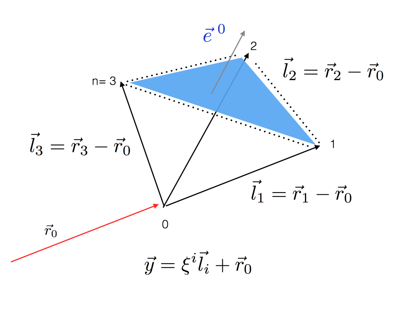
To pick a unique co-ordinate system on , we may eliminate one . for example and set so the flat metric tensor is given by .
Now the action22 2 Note on a flat simplex there is a single tangent plane with providing co-ordinates for all points, , in the interior. on each simplex in () is uniquely determined by Eq. 2 on this simplicial Riemann manifold
| (6) | |||||
where now with volume of the D-simplex and is the inverse of the metric tensor.


Finite Element Expansion:
The second step is to expand the field,
| (7) |
on each D-simplex into elements that contribute exclusively to one site: . For example, if we use linear elements, , in the interior and again eliminate, , the field on the simplex is
| (8) |
Using Eq. 6 and taking the gradient, , the integrand for the kinetic term in the action is a constant trivially giving
| (9) |
on each simplex. (The potential term, , in Eq. 6 is discussed in Sec. 3.) While this is the correct FEM kinetic term, one inconvenience is that our arbitrary choice of eliminating appears to break the symmetry between the sites. There is a symmetric treatment which has an appealing geometrical form. We introduce vierbeins normal to the surface opposite to each of the vertices (Fig. 2 ). These are not linearly independent because
| (10) |
but the gradient in this over-complete basis of tangent vectors is well defined,
| (11) |
and re-evaluating the action we get a symmetric form,
| (12) |
as a sum over all links on each simplex. This is exactly equivalent to Eq. 9 using the identity Eq. 10. More interestingly this identity (10) also gives the Laplace operator in link form on the RHS of Eq. 12. An alternative ansatz for this operator was introduced in Ref. [7] in terms of the dual simplex as
| (13) |
where is the product of the length of the link () times the surface volume () of the dual polytope normal to the link . That is , using the Hodge star of the discrete exterior calculus 33 3 The use of the discrete exterior calculus for forms, dual vectors, etc is a useful approach but the careful implementation of this formalism is difficult in a short review.. This geometrical form (13) suggested in Ref. [7] is very appealing but with the exception of it is not equivalent to linear finite elements (12) introduced in both the Regge and FEM literature. For , it may in fact be superior. This is one of many instances where a direct application of linear finite elements is either inadequate or at least may not be optimal for quantum field theory.
2.1 Laplacian on Riemann Sphere
We have tested the finite element construction of the Laplacian on the 2D Riemann sphere, . The isometric embedding of into is a sufrace with . For our simplicial lattice, we begin with an icosahedron and subdivide each of the 20 triangular faces into a regular grid of triangles as illustrated in Fig. 3. There are a total of vertices, edges and faces satisfying Euler’s theorem for a spherical topology .
We then project radially the sites of the refined icosahedron onto the unitsphere in and set the lengths of the edges to the secant distances, . This defines our simplicial Riemann manifold which is a good approximation to the sphere that preserves the icosahedral subgroup exactly, but the individual triangles are no longer regular. The spectrum of the resultant FEM Laplacian matrix converges as to the continuum values as illustrated in Fig. 4.
3 Interacting Scalars
After testing the spectrum for the free scalar, there remains the question of how to formulate interacting field theories.
As our first test, we drop the radial (time) direction in the 2+1 dimensional radially quantized theory. In the continuum, this example is equivalent to the stereographic projection of the Ising (c=1/2 minimal model) CFT from to . Since this map on the Riemann sphere is conformal up to a Weyl rescaling, all correlation functions are computable analytically at the fixed point, providing an ideal rigorous test of convergence to the continuum.
Our FEM partition function is given by
| (14) |
where for the kinetic term we used weights, , in Eq. 13. For the potential term, we use a local approximation to FEM integral, as opposed the weighted average of the mass term discussed in Sec. 5.1. The local weight, , is the dual Delaunay volume at . This approximation is equivalent to dropping irrelevant higher dimensional operators in a renormalizable quantum field theory. Monte Carlo simulations for this action are extremely efficient using the Brower-Tamayo form [10] of the Wolff Cluster algorithm [11].
Our first test of this was disastrous! Evaluating the Binder cumulant,
| (15) |
we attempted to find the critical surface by tuning at fixed in the continuum limit, , as illustrated on the left in Fig. 5. For moderate , the Binder cumulant appears to stabilize close to the analytical value [12] of , however as we approached closer to the continuum at large , it completely destabilized. On the right in Fig. 5, we see the explanation. The ensemble average, , has large low mode distortions. We see that the regions near the original 12 poles of the icosahedron and the region at triangular faces of the icosahedron appear to go critical at different values of . There is no critical surface with the Wilson-Fisher fixed point. The conventional FEM action (14) fails for quantum field theory.

3.1 Counter Terms for QFE
The problem with FEM for quantum field theory is fundamental. Although the proper use of FEM does guarantee convergence for the classical equations for smooth solutions on any scale well separated from the lattice spacing (or inverse ultraviolet cut-off ), the quantum field path integral samples all scales with divergent contributions in the ultraviolet (UV). Since the lattice is not quite regular, each lattice point has a slightly different UV cut-off . Fortunately in 2D, the theory is super-renormalizabie with the UV divergence occuring only in the one-loop graph on the left of Fig. 6. On the lattice this one loop diagram can be computed from our free lattice propagator by inverting the kinetic term matrix,
| (16) |
choosing to fix the physical mass scale independent of the cut-off.
On the 2D Riemann sphere, we find the one loop divergent term,
| (17) |
depends on an effective position dependent lattice spacing . This surprising result deserves a comment. As expected, the graph is logarithmically divergent in the cut-off , however fortunately the FEM prescription has removed the spatial dependence for the overall coefficient of the log divergence in the term. The “charge” is not renormalized and is given by its exact continuum result. Thus to cancel the UV spatial dependence in FEM quantum Lagrangian, we can subtract a finite counter term: ,
| (18) |
Indeed this finite term is almost precisely given by the log of the conformal scaling that mapped the flat faces of icosahedron onto the sphere. With this correction we arrive at our QFE simplicial Lagrangian, which now approaches the correct continuum CFT governed by the universal Wilson-Fisher fixed point in the continuum as illustrated in Fig. 7. This is an essential and significant success. The resultant QFE Lagrangian must include this quantum effect. In a future publication, we will report more generally on this critical step of determining the counter term. The 3D theory which is also super-renormalizable, has 2 divergent diagrams in Fig. 6 remormalizing the bare mass term. A very similar construction of counter terms appears to apply to the 3D radial theory which we are beginning to test numerically. Other approaches to counter terms are under investigation. For example the Pauli-Villars approach appears to provide a more general method for renormalizable field theories with the exception of non-Abelian gauge theories.
Binder Cumulants of QFE Theory:
We have tested our QFE 2D theory on a variety of exact correlation functions for this c=1/2 CFT. Here we report one such test, the Binder cumulants, to support our claim that the counter term has solved the problem of reaching the correct Wilson-Fisher fixed point for the c = 1/2 CFT. In particular high precision simulations up to sites on the Riemann sphere determined the critical surface at to be providing an evaluation of the Binder cumulant to be in statistical agreement with the analytic value of .
A series of higher order Binder cumulants [13] were used to provide an effective way to determine the critical surface.
The Binder cumulants are moments of the magnetization where . The lowest Binder cumulant, and higher cumulants are in general linear combinations of scale invariant magnetization ratios.
| (19) | |||||
As we approach the critical surface, we parameterized the Binder cumulant with a truncated expansion around the critical point,
| (20) |
We fixed and use the known critical exponents and . Then we tune to find the critical surface as can be seen in Fig. 7. The explicit fitting is done via simultaneous fits to all cumulants with common . Because this is a truncated expansion, one must be careful to only select data such that higher order terms in the expansion can be ignored.
As seen in Fig. 7, the value of the Binder cumulant can change drastically even at . Nevertheless, we are able to compute the first 5 Binder cumulants. These fits all have , giving numerical predictions for the analytically computable cumulants .
| 0.851003(8) | 0.8500(3) | 0.7724(4) | 0.7072(6) | 0.6483(8) | 0.5944(8) |
|---|
Analytical values for higher Binder cumulants are not yet available for comparison.
4 Dirac Fermions on Simplicial Lattice
Further subtleties are encountered for the discretization of Dirac and Gauge fields that carry spin. The Dirac field on a Riemann manifold,
| (21) |
is particularly subtle since it requires two new structures to deal with half integer spin: i.) The components of the tangent vector , where is the inverse of entering into the metric. ii.) The spin connection , where are the Lorentz generators for the Dirac spinors. The action is invariant under diffeomorphism or the choice of co-ordinates for the manifold. In addition there is a local “gauge” invariance allowing an arbitrary rotation (or Euclidean Lorentz transformation) in the tangent planes: at . This acts on the spinors as a gauge invariance in the Spin(D) covering group. The spin connection and the vierbeins are related by the tetrad postulate,
| (22) |
On a flat manifold the spin connection is a pure gauge and can be set to one by choosing a global tangent plane but on a curved manifold this is not possible. Indeed not all manifolds admit a spin structure. 44 4 Apparently a spin structure on a vector bundle E exists if and only if the second Stiefel-Whitney class vanishes. The special subtlety of placing the Dirac equation on a simplicial lattice is to provide a lattice realization of this spinor geometry.
Our construction introduces a compact spin gauge link, in the spinor covering group of the Euclidean Lorentz group and a lattice “vierbeins” which are tangent vectors contracted with the gamma matrix at site on the outgoing geodesic from to as depicted in Fig. 8. On the lattice we choose these tangent vectors to have unit length: . The naive kinetic term in the lattice Dirac action,
| (23) |
is anti-hermitian by virtue of . A Wilson term will be added to remove doublers. The Dirac operator in Eq. 23 is manifestly gauge invariant by virtue of
| (24) |
One can motivate this ansatz by starting from flat space with and make an arbitrary spinor rotations () to reorient the tangent vectors to derive this parameterization with the spin connection, , as a pure gauge. We should also note that, by generalizing the ansatz in Ref [14], our Fermion lattice action is not given by expanding the field in linear FEM even for 2D in flat space. In general linear elements fail to give “verbeins” parallel to the links. However in 2D, we have been able to remedy this by inventing a new Dirac QFE basis formed from 3 flat sub-triangles meeting at the dual site (or circumcenter) of each triangle. This construction reduces exactly to our action (23) for a flat 2D manifold as will be demenstrated in Ref. [9].
4.1 Spin Connection
Now we must construct explicitly the lattice spin connection and “vierbein” on the simplicial manifold () that conforms to the target continuum Riemann manifold (). The first difficulty with our simplicial complex is the assumption that the interiors of each simplex is flat, which implies curvature singularities at the vertices. In general to deal with the lack of a well defined tangent plane at the vertices, in Regge Calculus the Fermions are usually placed on the dual lattice sites [15] at the circumcenter of each simplex. However, this solution is troublesome for our goal of simplicial lattice field theory. With gauge fields on links, matter fields (scalar and Dirac) must be on sites to maintain gauge invariance. Our solution is to construct the spin links assuming a new simplicial manifold without these curvature singularities prior to introducing elements linear or higher order for the action. For example on the sphere the solution is to remove the singular curvature at the sites by replacing the links by geodesics (great circles in 2D) and the simplices by spherical elements describe in Sec 5. This hybrid approach is good to as demonstrated numerically on . A more general relaxation algorithm is also outlined below for a general simplicial complex that should converge on a sufficiently faithful approximation to a smooth Riemann manifold.

Naively, simply describes the rotation of a frame at (i) to a frame at (j). However, the Spin(D) group is a double cover of the Lorentz group . This manifests itself as a sign ambiguity in lifting to the spinor representation, . To fix this ambiguity, we look at the integrated curvature invariant associated with going around each triangular simplex. The algorithm as illustrated on the left in Fig. 8 proceeds in 3 steps: i.) Choose a random tangent frame at and align the tangent vectors at site on the geodesic from to all neighboring sites . ii.) Parallel transport the frame from to along a geodesic and compute the Lorentz rotation to the frame of . iii.) Map to the double cover in and choose the sign, to minimize the integrated curvature on the triangle: consistent with the area of the triangle, , vanishing in the continuum limit.
Choosing is a global constraint. We can iterate fixing the signs, , on each triangle in order to satisfy . These signs are shared by adjacent triangles, so this procedure will either produce a specific spin connection or fail to find a solution, if the manifold does not admit a spin structure. For example on the sphere one can choose to expand the path one triangle at a time until we reach the last triangle. Now the total enclosed deficit angle on a sphere is steradians so the last small triangle has the right sign automatically satisfied. Incidentally this follows essentially from Euler’s theorem. Higher genus 2D surfaces have solutions. For example for the 2 torus, , this procedure will lead to one of 4 different spin structures with period vs anti-periodic boundaries on the two non-contractible loops, referred to as Neveu-Schwarz/Neveu-Schwarz, Neveu-Schwarz/Ramond, Ramond/Neveu-Schwarz and Ramond/Ramond respectively in string theory. In the language of category theory, the existence of a spin structure is a property shared between any simplicial complex and Riemann manifolds to which they correspond.
The above procedure requires calculating the geodesic from each site to its neighboring sites to determine the angles between the tangent vectors. For spherical geometry this is a straightforward procedure because geodesics are known a priori to be great circles. For more complicated surfaces, calculating geodesics and performing parallel transport can be a difficult task and a more general method is preferable. An alternative is to use a relaxation approach to match the lattice action to the continuum. Here we sketch the approach, with details of the implementation given in a future article. We begin by introducing as free parameters to be fixed via a global minimization, comparing the local curvature in at each vertex to the lattice approximation. To do this we compare the continuum curvature at to the parallel transport around each adjacent triangle :
| (25) |
where the oriented area is defined by and the local curvature tensor by at site . To enforce this correspondence, one can simply minimize a quadratic form,
| (26) |
by a procedure familiar to gauge fixing in lattice field theory. This step has assumed a particular frame for the tangent planes, so now we need to find the tangent vectors in that frame. To do this, we recompute the curvature as function of the vectors on each triangle as illustrated Fig. 8 on the right, assuming our values of and the constraint: . Parallel transport anti-clockwise on a triangle has rotation matrices,
| (27) |
At each vertex, the angle, , rotates into , as illustrated in Fig. 8. Thus we can subsequently fix the “vierbein” by minimizing an appropriate form such as
| (28) |
varying at fixed . The result should determine “vierbein” on each tangent plane up to an overall irrelevant global rotation. Numerical tests and alternative algorithms for this relaxation procedure are under investigation.
4.2 Doublers and Chiral Symmetry
Next we must deal with the usual issue of doublers and chiral symmetry for lattice fermions. In the lattice Dirac theory on a flat manifold, the doublers can be removed by adding the Wilson term. In a non-Abelian gauge theory, the square of the Dirac operator,
| (29) |
is a sum of two terms which are referred as the Wilson term and the clover term respectively, when placed on the lattice. Similarly the square of the spinorial Dirac operator on a curved manifold is a linear combination of two similar terms,
| (30) |
where . On our simplicial complex, the first term will become our Wilson operator on a curved manifold,
| (31) |
and the second term is the lattice curvature in the spinor basis. Before utilizing this Wilson term on curved manifolds, it is interesting to see its effect on a flat 2D triangular lattice. As depicted in Fig. 9, in absence of the Wilson term, the hexagonal Brillouin zone in 2D on a triangular lattice actually has 6 copies of the 2 component spinor, but when the Wilson term is added the doublers are removed and the spectrum comes close to the circular complex spectrum of a lattice overlap operator.
Not surprisingly the qualitative effects on are very similar. We should also note that this Wilson term can be used to introduce Domain Wall Fermions on a simplicial complex with an extra flat dimension to restore chiral symmetry.
4.3 Spectral Analysis
Numerical tests of the simplicial Dirac framework on a have been performed which demonstrate convergence to the exact continuum spectra [16] as a function of the square of the average lattice spacing, , in Fig. 11.
The continuum Dirac operator, , on is anti-hermitian with Hermiticity: for D = 2. The spectrum is gapped, with eigenvalues with degeneracy for total angular momentum . Chiral fermoins on a sphere have no zero mode. The size of the gap scales inversely to the radius of the . The Euclidian continuum theory also admits a parity/time-reversal symmetry ( respectively) with the product being charge-conjugation symmetry.
We can now build a Dirac-Wilson operator described by Eq. 21 and analyse its spectrum. The results for can be seen in Fig. 10. The full shape of the spectrum is reminiscent of the arc-like shape seen for fermions on a flat triangular lattice. As the arc gets steeper for small-norm eigenvalues approach the continuum result as seen in Fig. 10. The real part of the spectrum, which determines this arc’s shape, is determined by the Wilson term. As the Wilson term is turned off, the eigenvalues collapse on the imaginary line but suffers from doublers.
We find that the first 3 levels of eigenvalues are exactly degenerate—corresponding to the protected icosahedral symmetry. Further, the symmetries are preserved on the lattice. The lattice eigenvalues approach the continuum as . For example, if we look at the imaginary part for (the lowest multiplet not protected by icosahedral symmtry), it approaches the continuum as . The Wilson term contains an extra factor of lattice spacing and thus vanishes more slowly as at the fourth eigen-level. We have also checked that the eigenvectors of our lattice Dirac operator converge to the analytic continuum wave function for the Dirac equation on . This is accomplished by a rotation of the gauge from our random tangent planes to be aligned with the continuum solution in the frame [9].
5 Spherical Finite Elements
As we mentioned in our application to the Dirac action on , we assumed a spherical simplicial lattice for the purpose of fixing the spin connection. This naturally leads us to consider if spherical elements could be constructed as a FEM basis. Although an explicit construction is unnecessary, alternative discretization schemes are interesting in their own right as possible improvement schemes designed to accelerate convergence to the continuum.
Here we show that on , it is indeed possible to design a finite element using spherical triangles whose boundaries are the geodesics of the sphere. We compute the spherical finite elements using a method which we call the “renormalization group approach,” and argue that it may be applied to more general manifolds and to theories which are not conformal. We also mention a second approach to computing the spherical elements based on the Riemann mapping theorem which is mathematically elegant although less general.
The finite element approach can be expressed as a decomposition of the continuum action into a sum over disjoint integration domains,
| (32) |
For a scalar field, let us also assume that the domains in D-dimensions are defined by D+1 sites and the fields are determined by the value of the fields on the sites. To achieve this we need to establish unique boundaries between the domains following a natural generalization of the linear element in flat space. We define the edges () to be geodesics, a natural generalization of straight lines in flat space. For D ¿ 2, we ascend to higher dimensional boundary elements: minimal 2D surfaces () with fixed edges, minimal 3D volumes () with fixed surfaces, etc. Finally we define the elements to be the unique solution to Laplace’s equation with the given boundary data. This procedure guarantees that the general solution is a linear function of the fields on the sites
| (33) |
The elements are therefore solutions with and and the identity,
| (34) |
is guaranteed so the constant field is preserved. By design this prescription in flat space reduces to the linear FEM, , in terms of barycentric coordinates.
Once the weight functions are known, the integral over the functional of the elements defines the discrete massless kinetic term or Laplacian operator on each element,
| (35) |
We now we restrict our explicit construction to , although generalizations to other smooth Riemann manifolds should follow a similar approach.
Renormalization Group Approach:
Our task is to solve a classical field equation on a curved manifold with prescribed boundary values. This is exactly the kind of problem that a sequence of linear finite elements are designed to solve. If we refine the graph further, we break each spherical triangle element (in general a D-simplex) into a sequence of an increasing number of smaller spherical triangles, approximated with increasing accuracy by flat triangles with the linear finite element expression (12). All that remains is to numerically relax the lattice field variables to the configuration which minimizes the action. We perform the relaxation using the conjugate gradient algorithm.
This procedure can be interpreted as a renormalization group flow in the sense that we are replacing an action expressed in terms of many linear finite elements at short distance with an action of equal value expressed with spherical finite elements at long distance. We are not integrating out degrees of freedom as is done in a usual real space RG procedure, but our theory is gaussian so there are non-linearities to take into account. This approach is not limited to the Riemann sphere. In general, one should be able to construct a “geodesic triangular element” on a manifold by laying down a simplicial mesh on the geodesic element and solving for the classical solution of Laplace’s equation on the curved space using linear finite elements.
Conformal Mapping Approach:
The conformal mapping approach makes use of two mathematical identities to simplify the problem and to avoid computing the elements directly. The first identity uses conformal mapping to express the action on a triangle as an integral over the unit disk in the complex plane. The mapping takes place in three steps. First, stenographically project the spherical triangle onto the flat complex plane with a triangular image bounded by 3 circular arcs. Second, use the Schwartz triangle function [17] (a generalization of the Schwarz-Christoffel transformation for circular arc polygons) to map the circular arc triangle onto the upper half plane. Third, use the Möbius transformation to map the upper half plane onto the unit disk. Only the Schwartz triangle map is nontrivial, involving ratios of hypergeometric functions that map the linear interpolation of the geodesics on the spherical triangle to non-uniform distributions on the boundaries of the disk with singularties at the vertices. Nonetheless, the interpolated boundary data, , on the unit circle can be computed numerically by a look up table on the original data.
The second identity uses the divergence theorem and Green’s theorem to rewrite the action as an integral over the boundary of the disk. First the divergence theorem expresses the action as boundary value problem,
| (36) |
since the second term vanishes by the equations of motion. Next we can use Green’s theorem to rewrite the solution in terms of the boundary values,
| (37) |
Combining these equations for the unit disk leads to a remarkable closed form as a double boundary intergral,
| (38) |
where is the inverse mapping function from the boundary of the unit disk back to the boundary of the spherical triangle. These integrations can be done numerically using a well constructed numerical adaptive integrator. The crucial feature in this identity (38) is the inclusion of local terms, and , in the integrand that renders it non-singular at . Our derivation of this “regulator” relied on the use of confromality and vertex functions for the bosonic string theory.
5.1 Spectrum of Spherical Finite Element Laplacian
When computing spectra of operators on curved manifolds, one must solve the generalized eigenvalue problem,
| (39) |
with eigenfunctions that are orthogonal with respect to the correct measure, . The discrete measure, , may be chosen in a variety of ways. One approach is to take the area at a site to be the area of the Voronoi dual cell. Another approach is to construct the finite element expression which gives a non-local mass term: . We refer to this as the finite element method (FEM) mass term. In our results, we consider four spectra: the flat finite element with Voronoi area term, the flat finite element with FEM area term, the spherical finite element with Voronoi area term, and the spherical finite element with FEM area term.
Fig. 12 is a plot of the complete set of eigenvalues against the principle quantum number for a refinement of . On the left plot, one sees a striking difference between the FEM area term and Voronoi area term. The spectrum with FEM area term converges from above, which corresponds to a suppression of high angular momentum degrees of freedom at finite lattice spacing, while the spectrum with Voronoi area term converges from below, which corresponds to an enhancement of high angular momentum degrees of freedom. The right plot compares the spherical element and flat element spectra, which are essentially the same, so on this plot they merge into single circles one on top of the another.
Fig. 13 demonstrates the convergence of the eigenvalues for as the lattice spacing is taken to zero for our spherical finite element. ( Of course a very similar plot holds for the linear finite elements spectra.) In the left plot, we show the error of the level mean from the eigenvalues relative to the exact continuum value of . In the right plot we show the standard deviation of the splitting of the eigenvalues relative to their mean. Both plots are plotted against the refinement, , on a log-log scale to demonstrate convergence as for sufficiently large .
Finally, we note that because of the conformality of the 2D free Laplacian, it is possible to re-interpret the spherical element as a new element mapped onto the original flat simplicial complex. On each spherical triangle, the radial projection from the barycentric co-ordinates to the spherical co-ordinates, , maps the secants to great circles and the metric is given by the flat metric in Eq. 6, up to a conformal factor: . In 2D, the conformal factor cancels in so we have the identity,
| (40) |
Consequently the spherical elements are equivalent to a new element basis on the simplicial complex with flat triangles, conforming to linearity in arclength on the projected great circles. In higher dimensions the conformal factor does not cancel, so one cannot interpret the spherical elements in this way; nonetheless they may still be constructed and used as elements on the original manifold.
6 Conclusion
We report on a new formulation of lattice field theory suited to smooth Riemann manifolds. The 2D scalar field theory on the Riemann sphere is now under control at the Wilson-Fischer fixed point. The accuracy of the Binder cumulants is comparable to previous numeric and analytic results. The numerical precision was dependent upon correcting the linear finte elements by a one loop counter term explicitly evaluated on the simplicial complex. The foundation for Dirac fermions on simplicial lattices has also been laid down. The spectrum and wavefunctions for free scalars and Fermions were numerically show to converge to the continuum as expected for the Riemann sphere.
For the both the scalar and the Dirac simplicial lattice actions, we note that strict adherence to linear FEM is not effective. Instead we sought a new formulation which we refer to as QFE for Quantum Finite Elements. While we report only on numerical tests on the Riemann sphere, the basic methods will apply more generally. We have now developed all the necessary tools and software to test QFE on the radial quantization of the 3D Ising CFT at the Wilson-Fisher fixed point. In the future we will include non-Abelian gauge theories. We anticipate no fundamental barriers for super renormalizable field theories but asymptotically free gauge theories in 4D will most likely require more fundamental advances. On the software level, we plan to extend the SciDAC data parallel software for Lattice Field Theory to simplicial lattices, clearly a prerequisite to robust numerical simulation for a large range of applications to the physics of quantum fields on curved manifolds.
Acknowledgments
R.C.B acknowledges useful discussions with John Cardy, Ami Katz and Martin Lüscher. R.C.B. and E.W. were supported by DOE grant DE-SC0010025. R.C.B. and G.F. thank the Aspen Center for Physics, which is supported by National Science Foundation grant PHY-1066293 and thank the KITP, Santa Barbara, supported in part by the National Science Foundation under Grant No. NSF PHY11-25915.
References
- [1] R. Brower, G. Fleming, and H. Neuberger, Lattice Radial Quantization: 3D Ising, Phys.Lett. B721 (2013) 299–305, [arXiv:1212.6190].
- [2] R. C. Brower, M. Cheng, and G. T. Fleming, Improved Lattice Radial Quantization, PoS LATTICE2013 (2014) 335, [arXiv:1407.7597].
- [3] R. C. Brower, M. Cheng, and G. T. Fleming, Quantum Finite Elements: 2D Ising CFT on a Spherical Manifold, PoS LATTICE2014 (2015) 318.
- [4] T. Regge, GENERAL RELATIVITY WITHOUT COORDINATES, Nuovo Cim. 19 (1961) 558–571.
- [5] N. Christ, R. Friedberg, and T. Lee, Random Lattice Field Theory: General Formulation, Nucl.Phys. B202 (1982) 89.
- [6] N. H. Christ, R. Friedberg, and T. D. Lee, GAUGE THEORY ON A RANDOM LATTICE, Nucl. Phys. B210 (1982) 310.
- [7] N. H. Christ, R. Friedberg, and T. D. Lee, Weights of Links and Plaquettes in a Random Lattice, Nucl. Phys. B210 (1982) 337.
- [8] G. Strang and G. Fix, An Analysis of the Finite Element Method 2nd Edition. Wellesley-Cambridge, 2nd ed., 5, 2008.
- [9] R. Brower, G. Fleming, A. Gasbarro, T. Raben, C.-I. Tan, and E. Weinberg, Lattice Dirac Fermions on a Curved Manifold, in preperation.
- [10] R. Brower and P. Tamayo, Embedded Dynamics for Theory, Phys.Rev.Lett. 62 (1989) 1087–1090.
- [11] U. Wolff, Collective Monte Carlo Updating for Spin Systems, Phys.Rev.Lett. 62 (1989) 361.
- [12] Y. Deng and H. W. Blote, Conformal invariance and the Ising model on a spheroid, Phys.Rev. E67 (2003) 036107.
- [13] K. Binder, Critical Properties from Monte Carlo Coarse Graining and Renormalization, Phys. Rev. Lett. 47 (1981) 693–696.
- [14] R. Friedberg, T. D. Lee, and H.-c. Ren, FERMION FIELD ON A RANDOM LATTICE, Prog. Theor. Phys. Suppl. 86 (1986) 322.
- [15] H. W. Hamber, Quantum Gravity on the Lattice, Gen.Rel.Grav. 41 (2009) 817–876, [arXiv:0901.0964].
- [16] A. A. Abrikosov, Jr., Dirac operator on the Riemann sphere, hep-th/0212134.
- [17] Z. Nehari., Conformal Mapping., McGraw-Hill, New York.