Density of 4-edge paths in graphs with fixed edge density

We will use the following notations. $I_{i}=[q_{i-1},q_{i})$, $t_{i}=q_{i}-q_{i-1}=|I_{i}|$, $\ell_{i}=\ell(x)$ for any $x\in I_{i}$, $A_{i,j}$ is the value of $A$ in the rectangle $I_{i}\times I_{j}$. We will refer to the sets of the form $[0,1)\times I_{i}$ and $I_{i}\times[0,1)$ as rows and columns respectively.

The function $S$ is continuous on a compact set defined by the conditions, so its maximum is attained for some $A$. Let $A$ be a function maximizing $S$, and let

By a similar compactness argument, the minimum of $T$ is also attained for some $A$ (among those that maximize $S$). Such an $A$ can not have four rectangles $I_{i_{1}}\times I_{j_{1}},I_{i_{1}}\times I_{j_{2}},I_{i_{2}}\times I_{j_{1}}$ and $I_{i_{2}}\times I_{j_{2}}$ satisfying $A_{i_{1},j_{1}}<A_{i_{2},j_{1}}$ and $A_{i_{1},j_{2}}>A_{i_{2},j_{2}}$.

For some $\varepsilon>0$, replace the values $A_{i_{1},j_{1}},A_{i_{2},j_{1}},A_{i_{1},j_{2}}$ and $A_{i_{2},j_{2}}$ by $A_{i_{1},j_{1}}+\frac{\varepsilon}{t_{i_{1}}t_{j_{1}}},A_{i_{2},j_{1}}-\frac{\varepsilon}{t_{i_{2}}t_{j_{1}}},A_{i_{1},j_{2}}-\frac{\varepsilon}{t_{i_{1}}t_{j_{2}}}$ and $A_{i_{2},j_{2}}+\frac{\varepsilon}{t_{i_{2}}t_{j_{2}}}$ respectively. By choosing a small enough $\varepsilon$, the value of $A$ remains greater in $I_{i_{2}}\times I_{j_{1}}$ and $I_{i_{1}}\times I_{j_{2}}$ than in $I_{i_{1}}\times I_{j_{1}}$ and $I_{i_{2}}\times I_{j_{2}}$ respectively. Note that such a change does not change the values $\ell(x)$, therefore not changing $S(A)$. (To see that, take a line that intersects two of the four rectangles where the value of $A$ changes. It increases in one of them, while decreasing in the other one. This results in a 0 net change in the integral of $A$ over that line, since if one of the rectangles intersect the line in a segment $\lambda$ times as long as the other one, then its area is $\lambda$ times greater, so the change in the value of $A$ is $\lambda$ times smaller.)

Now we show that the value $T(A)$ decreases during this transformation. $T(A)$ is the sum of differences between the values $A_{i,j}$, weighted with the areas of these rectangles. Assume that the value of $A$ is greater in $r_{1}$ than in $r_{2}$ for two rectangles $r_{1}$ and $r_{2}$. If we decrease the value of $A$ in a rectangle $r_{1}$ with $\frac{\varepsilon}{Area(r_{1})}$, and increase it in $r_{2}$ with $\frac{\varepsilon}{Area(r_{2})}$ for a small enough $\varepsilon$, then $T(A)$ decreases. To see that, note that

and for any rectangle $r_{3}\not\in\{r_{1},r_{2}\}$

Applying this to $(r_{1},r_{2})=(I_{i_{2}}\times I_{j_{1}},I_{i_{1}}\times I_{j_{1}})$ and $(r_{1},r_{2})=(I_{i_{1}}\times I_{j_{2}},I_{i_{2}}\times I_{j_{2}})$ the desired result follows.

The symmetry of $A$ can be ruined by this transformation, but replacing $A(x,y)$ by $\frac{A(x,y)+A(y,x)}{2}$ for all $0\leq x,y\leq 1$ fixes this while not increasing $T(A)$ and not changing $S(A)$. (The fact that $T(A)$ does not increase can be verified by the above calculation dealing with the decrease of $A$ in a high-valued rectangle and the its increase in a lower valued one.)

Rearrange the intervals $I_{i}$ such that $\ell_{1}\geq\ell_{2}\geq\dots\geq\ell_{K}$. The property we just proved for the rectangles implies that for any four rectangles of the form $I_{i_{1}}\times I_{j_{1}},I_{i_{1}}\times I_{j_{2}},I_{i_{2}}\times I_{j_{1}}$ and $I_{i_{2}}\times I_{j_{2}}$, we have

Now we prove that $A$ is decreasing in both variables. (Since $A(x,y)=A(y,x)$, it is enough to show that for one variable.) Assume to the contrary that for some $i_{1}<i_{2}$ and $j$ we have $A_{i_{1},j}<A_{i_{2},j}$. Then for all $1\leq p\leq K$ we have $A_{i_{1},p}\leq A_{i_{2},p}$. It results in $\ell_{i_{1}}<\ell_{i_{2}}$, a contradiction.

This decreasing property implies that if $\ell_{i}=\ell_{i+1}$ then $A$ is identical in $I_{i}\times[0,1)$ and $I_{i+1}\times[0,1)$ so we can merge all such intervals and assume that $\ell_{1}>\ell_{2}>\dots>\ell_{k}$ for some $k\leq K$.

Note that $S(A)$ can be expressed as

Consider an $A$ that meets the theorem’s requirements, maximizes $S(A)$ and is decreasing in both variables. We state that there can not be two rectangles in the same row (or column) where the value of $A$ is neither 0 nor 1. Assume that for some $1\leq a<b\leq k$ and $1\leq p\leq k$ we have $0<A_{a,p}<1$ and $0<A_{b,p}<1$. Pick some $\epsilon\in\mathbb{R}$ and change $A_{a,p}$ and $A_{p,a}$ to $A_{a,p}+\frac{\varepsilon}{t_{a}t_{p}}$ while changing $A_{b,p}$ and $A_{p,b}$ to $A_{b,p}-\frac{\varepsilon}{t_{b}t_{p}}$. This transformation changes only two $\ell$ values: $\ell_{a}$ becomes $\ell_{a}+\frac{\varepsilon}{t_{a}}$ and $\ell_{b}$ becomes $\ell_{b}-\frac{\varepsilon}{t_{b}}$. If $|\varepsilon|$ is small enough then $0<A_{a,p}+\frac{\varepsilon}{t_{a}t_{p}},A_{b,p}-\frac{\varepsilon}{t_{b}t_{p}}<1$ and the order of the $\ell$ values is preserved. Now we show that $S(A)$ is a strictly convex function of $\varepsilon$ in a neighborhood of 0. Consider the $k^{2}$ terms in the expression (1). The terms including other terms than $a$ and $b$ are obviously convex functions of $\varepsilon$, since $\varepsilon$ appears at a power of at most 2 in them, and it has a positive coefficient when it has power 2. So the terms of $S(A)$ corresponding to pairs of indices other than $(a,a),(a,b),(b,a)$ and $(b,b)$ are convex functions of $\varepsilon$. All we have to prove is that the sum of the terms corresponding to these four pairs is strictly convex at $\varepsilon=0$.

Differentiating twice with respect to $\varepsilon$ and substituting $\varepsilon=0$, we get

It is positive, because $a<b$ implies $\ell_{a}>\ell_{b}$. Therefore $S(A)$ is a strictly convex function of $\varepsilon$ in a neighborhood of 0, so can not have a maximum at 0. This proves that the $A$ under investigation has at most one rectangle in every row and column with a value different from 0 or 1, as depicted in Figure 2.

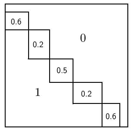
Now we will prove that actually there are no such rectangles at all. Since $A$ is decreasing in both variables, each row (and column) starts with some 1-valued rectangles, then it might include a single rectangle with value between 0 and 1, then it contains 0-valued rectangles. (Of course, a row or column not necessarily contains all three types of rectangles.) If $A$ has a single rectangle of size $t\times t$ with nonzero value, then $A$’s value is $\frac{c}{t^{2}}$ there. (So $\frac{c}{t^{2}}\leq 1$.) Then $S(A)=t^{2}\cdot(t\cdot\frac{c}{t^{2}})^{3}=\frac{c^{3}}{t}\leq c^{\frac{5}{2}}$. If there are multiple nonzero-valued rectangles, then $A_{1,1}=1$.

Assume that $0<\lambda=A_{1,j}=A_{j,1}<1$ for some $j$. (Then $j\in\{k-1,k\}$). We will show that it is possible to modify $A$ to increase $S(A)$, so this case is not possible. (From now on we will modify the lengths of the intervals too, not just the value of $A$ in the rectangles.) Divide the interval $I_{j}$ into two intervals $I_{j^{\prime}}$ and $I_{j^{\prime\prime}}$ of length $t_{j^{\prime}}=\lambda\cdot t_{j}$ and $t_{j^{\prime\prime}}=(1-\lambda)\cdot t_{j}$ respectively. Then divide $I_{1}\times I_{j}$ into two rectangles of size $t_{1}\times t_{j^{\prime}}$ and $t_{1}\times t_{j^{\prime\prime}}$, and set $A$ to be 1 and 0 respectively in them. Modify $A$ in $I_{j}\times I_{1}$ similarly to keep $A$ symmetric.

After this modification, we will get $\ell_{j^{\prime}}=\frac{\ell_{j}}{\lambda}$ and $\ell_{j^{\prime\prime}}=0$. This means that the terms with $j^{\prime\prime}$ can be ignored in (1). The only terms to change in (1) are $t_{j}$ becoming $t_{j^{\prime}}=\lambda\cdot t_{j}$ and $\ell_{j}$ becoming $\ell_{j^{\prime}}=\frac{\ell_{j}}{\lambda}$. Since the power of $\ell_{j}$ is not smaller than the power $t_{j}$ in any term of (1), and greater than it in $t_{j}^{2}\cdot\ell_{j}^{3}$, the value of $S(A)$ increases by this modification. So we can assume that $A$ takes only 0 and 1 values in $I_{1}\times[0,1)$ and $[0,1)\times I_{1}$. To show that noninteger values are not possible in the other places, we need a technical lemma.

Note that the variables $t_{i}$ and $\ell_{i}$ appearing in the following lemma should be considered real numbers with no connection to any function $A:[0,1)^{2}\rightarrow[0,1]$, but the same notations are used, since the lemma will be applied in such settings.

Now we can continue the proof of the theorem. Assume that $A$ is not entirely 0-1 valued. Let $I_{p}\times[0,1)$ be the first column containing a rectangle with a value different from 0 and 1. We already proved that $p\geq 2$. Let $I_{p}\times I_{q}$ the unique rectangle in the $p$-th column with $0<A_{p,q}<1$. Since $A_{p,q}=A_{q,p}$, we know that $p\leq q$. We will show that $A$ admits the type of transformation described in Lemma 2.3, therefore does not maximize $S(A)$. We will describe transformations in each case that change only two neighboring $t$ values and the $\ell$ corresponding to one of them.

Case a: First, assume that $p<q<k$ and $A_{p-1,q+1}=1$. Then the rows $[0,1)\times I_{q}$ and $[0,1)\times I_{q+1}$ differ only in the $p$-th column. We can move the point separating the intervals $I_{q}$ and $I_{q+1}$, keeping $A_{p,q+1}=0$ while adjusting $A_{p,q}$ such that the integral of $A$ over the whole square remains unchanged. We apply these changes to the other side of the main diagonal to keep $A$ symmetric. During this transformation the only $\ell$ value to change is $\ell_{q}$. So Lemma 2.3 can be applied with $\alpha=q+1,\beta=q$.

Case b: Now assume that $p<q=k$ or $p<q<k$ and $A_{p-1,q+1}=0$. Then the columns $I_{p-1}\times[0,1)$ and $I_{p}\times[0,1)$ differ only in the $q$-th row. We can move the point separating the intervals $I_{p-1}$ and $I_{p}$, keeping $A_{p-1,q}=1$ while adjusting $A_{p,q}$ such that the integral of $A$ over the whole square stays the same. We apply these changes to the other side of the main diagonal to keep $A$ symmetric. During this transformation the only $\ell$ value to change is $\ell_{p}$. So Lemma 2.3 can be applied with $\alpha=p-1,\beta=p$.

Case c: Assume that $p=q<k$ and $A_{p-1,p+1}=1$. Then the rows $[0,1)\times I_{p}$ and $[0,1)\times I_{p+1}$ differ only in the $p$-th column. We can move the point separating the intervals $I_{p}$ and $I_{p+1}$, keeping $A_{p,p+1}=0$ while adjusting $A_{p,p}$ such that the integral of $A$ over the whole square stays the same. (We apply these changes to the the intervals defining the rows and columns simultaneously to keep $A$ symmetric.) During this transformation the only $\ell$ value to change is $\ell_{p}$. So Lemma 2.3 can be applied with $\alpha=p+1,\beta=p$.

Case d: Now assume that $p=q=k$ or $p=q<k$ and $A_{p-1,p+1}=0$. Then the columns $I_{p-1}\times[0,1)$ and $I_{p}\times[0,1)$ differ only in the $p$-th row. We can move the point separating the intervals $I_{p-1}$ and $I_{p}$, keeping $A_{p-1,p}=1$ while adjusting $A_{p,p}$ such that the integral of $A$ over the whole square stays the same. (We apply these changes to the the intervals defining the rows and columns simultaneously to keep $A$ symmetric.) During this transformation the only $\ell$ value to change is $\ell_{p}$. So Lemma 2.3 can be applied with $\alpha=p-1,\beta=p$.

References

- [1] R. Ahlswede, G.O.H. Katona, Graphs with maximal number of adjacent pairs of edges, Acta Math. Acad. Sci. Hungar. 32 (1978) 97-120.
- [2] N. Alon, On the number of subgraphs of prescribed type of graphs with a given number of edges, Israel J. Math. 38 (1981) 116-130.
- [3] N. Alon, On the number of certain subgraphs contained in graphs with a given number of edges, Israel J. Math. 53 (1986) 97-120.
- [4] B. Bollobás, A. Sarkar, Paths in graphs, Studia Sci. Math. Hungar. 38 (2001) 115-137.
- [5] B. Bollobás, A. Sarkar, Paths of length four, Discrete Mathematics 265 (2003) 357-363.
- [6] Z. Füredi, Graphs with maximum number of star-forests, Studia Scientiarum Mathematicarum Hungarica 27 (1992) 403-407.
- [7] R. Kenyon, C. Radin, K. Ren, L. Sadun, Multipodal Structure and Phase Transitions in Large Constrained Graphs, arXiv:1405.0599
- [8] L. Lovász, Large Networks and Graph Limits, American Mathematical Society (2012)
- [9] A. A. Razborov, On the Minimal Density of Triangles in Graphs, Combinatorics, Probability and Computing, 17 (2008) 603-618.