Rate Performance of Adaptive Link Selection in Buffer-Aided Cognitive Relay Networks

It has been established that cognitive radio [1], in which an unlicensed (secondary) user shares the spectrum of the licensed (primary) user, has great potential for alleviating spectrum scarcity. In particular, underlay cognitive radio networks, in which the secondary node transmits with power that is controlled carefully to ensure that the interference caused to the primary receiver is below an interference temperature threshold, has attracted great research interest [2]. However, the severe interference constraints imposed by the primary networks seriously limits the transmit powers, and thereby the rates that can be achieved in the secondary networks.

The advantages of using of a buffer equipped relay has been demonstrated [3]. In non-cognitive two-hop networks, using a buffered-relay, Madsen [3] demonstrated rate enhancement in fading channels by averaging the instantaneous rate over multiple time-slots for both the hops. Unlike [3], Bing [4] utilized two-hops of equal duration, so that the rate was limited by the weaker link. Recently, it has been demonstrated [5, 6, 7] that buffering with adaptive link selection, where either the source-relay or relay-destination link is judiciously selected for transmission, can harness a diversity of two with fixed-rate transmission, and increase the average rate by a factor of two as compared to a conventional buffered relay scheme with adaptive rate. Symbol error rate (SER) performance of such systems is analyzed in [8]. Intuitively, since the sources in cognitive radio networks are power-limited, the use of relays is well motivated. Also, all the techniques employed to improve performance of relays can be utilized [9].

In [10], an interference cancellation-based scheme is proposed where the primary and the secondary sources pick one buffer-aided relay each for two-hop transmission, and address power allocation issues. In [11], a throughput-optimal adaptive link selection policy is proposed for the secondary two-hop network. For underlay two-hop buffer-aided relay networks, a sub-optimal relay selection scheme is proposed in [12], and its outage performance is analyzed assuming only the peak interference constraint (ignoring the peak power constraint). In [13], an overlay secondary source maximizes its own rate in a link without relays, while assisting the primary to attain its target rate using causal knowledge of the primary message.

In this paper, assuming peak interference and peak power constraints on the secondary nodes, we develop closed-form analytical expressions for rate performance of a two-hop underlay network with a buffered relay. We compare rate performance of the adaptive link selection scheme with that of conventional buffered and unbuffered relays. To facilitate rate analysis, we first derive expressions for the joint complementary cumulative distribution function (CCDF) of the link selection parameter and the instantaneous SNR of the selected link. We demonstrate that buffering with adaptive link selection is most beneficial in severely power constrained scenarios typically encountered in underlay cognitive radio. Intuitively, this is because the interference constraints make the transmit power of the source and relay in the two-hop network random variables. This increases the variance of the SNRs of the two hops, which makes use of a buffer at the relay more important than in cooperative links. Since use of the cognitive paradigm is being explored for use in 5G systems, performance of link-level two-hop cognitive radio networks is of great interest to researchers and system designers[14][15]. This this paper, we restrict out attention to rate performance. In the longer version of this paper, we address symbol error rate and delay performance issues.

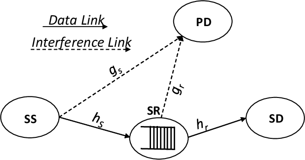
We consider a two-hop underlay cognitive network as depicted in Fig.1. The primary network consists of the primary destination (PD), and the secondary or unlicensed network consists of the secondary source (SS), the secondary destination (SD), and a half-duplex (HD) decode and forward (DF) secondary relay (SR). It is assumed that SR is equipped with a buffer. All secondary nodes are assumed to possess a single antenna. The SS-SD direct link is heavily shadowed, necessitating the use of a relay. All channels between nodes in this network are assumed to be quasi-static, and do not change in the signalling interval, though they change independently from slot to slot. The channel coefficients of the SS-SR and SR-SD links in a time-slot are denoted by $h_{s}$ and $h_{r}$ respectively, with $h_{i}\sim{\cal CN}(0,\Omega_{h_{i}}),i\in\{s,r\}$. The channel coefficients of the SS-PD and SR-PD interference links are denoted by $g_{s}$ and $g_{r}$ respectively, with $g_{i}\sim{\cal CN}(0,\Omega_{g_{i}}),i\in\{s,r\}$. Let $d_{sr}$, $d_{rd}$, $d_{sp}$ and $d_{rp}$ denote the SS-SR, SR-SD, SS-PD and SR-PD distances respectively. With a path-loss Rayleigh fading channel model, it is clear that $\Omega_{h_{i}}=d_{ij}^{-\alpha}$ and $\Omega_{g_{i}}=d_{{ip}}^{-\alpha}$ respectively, where $i\in\{s,r\},j\in\{r,d\}$, and $\alpha$ is the path-loss exponent. We also assume zero-mean additive white Gaussian noise of $N_{o}$ variance at all terminals.

Underlay CR nodes [16] use an interference constraint so that SS and SR restrict their instantaneous transmit power in order to limit the peak interference to PD below an interference temperature limit (ITL) ${\cal I}_{p}$. We assume that maximum transmit power at SS and SR is limited to $P_{max}$ (peak-power constraint), and define the system SNR as $\gamma_{max}=P_{max}/N_{o}$. With peak interference and peak power constraints, the instantaneous SNRs $\gamma_{i}$ are given by[16]:

$\displaystyle\gamma_{i}$

$\displaystyle=$

$\displaystyle\min\left\{\gamma_{max},\dfrac{\gamma_{p}}{|g_{i}|^{2}}\right\}|h_{i}|^{2},\quad i\in\{s,r\}$

(1)

where $\gamma_{p}={\cal{I}}_{p}/N_{o}$. The instantaneous capacity of the two hops is defined as $C_{i}=\log_{2}(1+\gamma_{i})$ $i=s,r$. In the low SNR regime referred to as the peak transmit power regime (PTPR), $\gamma_{max}$ is small (which ensures that $\gamma_{max}<<\gamma_{p}/|g_{i}|^{2},$) so that the link SNRs are determined solely by the peak power (and modelled as a exponential random variables). In the high SNR regime referred to as the peak interference power regime (PIPR), $\gamma_{max}>>\gamma_{p}/|g_{i}|^{2},$ so that the link SNRs are limited by the interference (and modeled as a ratio of exponential random variables). The probability $p_{i}$, $i\in\{s,r\}$ that the peak interference ($P_{max}|g_{i}|^{2}$) at PD with peak transmit power is higher than ${\cal I}_{p}$ is given by:

$\displaystyle p_{i}$

$\displaystyle=$

$\displaystyle\Pr\left\{\gamma_{max}>\dfrac{\gamma_{p}}{|g_{i}|^{2}}\right\}=e^{-{\mu_{i}}/{\lambda_{i}}},\quad i\in\{s,r\}$

(2)

where $\lambda_{i}=\gamma_{max}\,\Omega_{h_{i}}$ and $\mu_{i}=\dfrac{\gamma_{p}\Omega_{h_{i}}}{\Omega_{g_{i}}}$ are the average SNRs when the SS/SR transmits with $P_{max}$ and $\dfrac{\mathcal{I}_{p}}{\Omega_{g_{i}}}$ power respectively. Note that when the ratio $\dfrac{\mu_{i}}{\lambda_{i}}$ is $\infty$ and $0$, the corresponding probabilities $p_{i}$ are $0$ and $1$ respectively. Hence $p_{i}=0$ ($p_{i}=1$) indicates that the node $i\in\{s,r\}$ is operating in the PTPR (PIPR).

In literature [16], expressions have been derived for CDF of the SNRs $\gamma_{i}$ of (1) of the two links. We will find it convenient to write the CCDF and PDF of link SNRs $\gamma_{i}$ in terms of $p_{i}$ as follows:

	$\displaystyle\hskip-14.45377ptF_{\gamma_{i}}(s)\hskip-7.22743pt$	$\displaystyle=$	$\displaystyle\hskip-7.22743pt1-e^{-{s}/\lambda_{i}}\left[1-p_{i}\left(1-\dfrac{\mu_{i}}{s+\mu_{i}}\right)\right],$		(3)
	$\displaystyle\hskip-14.45377pt\hskip-72.26999ptf_{\gamma_{i}}(s)\hskip-7.22743pt$	$\displaystyle=$	$\displaystyle\hskip-7.22743pt\dfrac{e^{-{s}/\lambda_{i}}}{\lambda_{i}}\left[1-p_{i}\left(1-\dfrac{\mu_{i}}{s+\mu_{i}}-\dfrac{\lambda_{i}\mu_{i}}{(s+\mu_{i})^{2}}\right)\right].$		(4)

In the above, use of $p_{i}=0$ and $p_{i}=1$ results in expressions for PTPR and the PIPR cases respectively.

We assume that both SS and SR have required CSI. Further, they use adaptive modulation to transmit with maximum rate (the instantaneous capacity of the channel). For rate enhancement, we incorporate the dual-hop adaptive link selection relay scheme of [5],[7], where the SS-SR or SR-SD link, whichever has higher capacity, is chosen so as to attain good performance (while ensuring buffer stability). For analytical tractability (as in [5],[7]), the suboptimal decision function based on the ratio of instantaneous SNRs $\gamma_{s}$ (SS-SR link) and $\gamma_{r}$ (SR-RD link) is used:

$$d=\left\{\begin{array}[]{l l}1&\quad\text{if $\dfrac{\gamma_{r}}{\gamma_{s}}\geq$}\rho\ (\text{SR transmits})\\ 0&\quad\text{otherwise (SS transmits)},\end{array}\right.$$

(5)

where $d$ is the one-bit link-selection parameter, and $\rho$ is a positive statistical parameter that depends on average channel gains. $\rho$ is chosen to maximize rate while ensuring buffer stability. We assume that SS always has data to transmit, and that SR has an infinite-sized buffer and choose $\rho$ such that the rate is maximised. Hence the average rate of ALSBR is:

$\displaystyle\overline{{\mathcal{R}}}^{ALSBR}=\mathbf{\E}_{\gamma_{s},\gamma_{r}}[dC_{r}]=\mathbf{\E}_{\gamma_{s},\gamma_{r}}[(1-d)C_{s}].$

(6)

where $\mathbf{\E}_{X}\{.\}$ denotes expectation over the variable $X$. To choose a link, the ALSBR scheme needs the instantaneous SNRs of the two links together with some average channel gains. We assume that the relay node (using transmitted pilots), performs this selection, and communicates the same to SS prior to signalling in each time-slot.

In this paper, we compare performance of the ALSBR scheme with the conventional unbuffered relay (CUBR), which holds the single packet in unit length buffer before relaying it in the next time-slot. The average rate of CUBR is given by[3]:

$\displaystyle\begin{array}[]{lll}\overline{{\mathcal{R}}}^{CUBR}=1/2\,\mathbf{\E}_{\gamma_{s},\gamma_{r}}[\min\{C_{s},C_{r}\}].\end{array}$

In the conventional buffered relay (CBR) scheme that we also use for comparison, the data is stored (hence averaged) for multiple slots before relaying to SD. These slots are equal for SS-SR and SR-SD links, which ensures that the average rate of CBR is [4]:

$\displaystyle\begin{array}[]{lll}\overline{{\mathcal{R}}}^{CBR}=1/2\,\min\{\mathbf{\E}_{\gamma_{s}}[C_{s}],\mathbf{\E}_{\gamma_{r}}[C_{r}]\}.\end{array}$

The CCDF $F^{c}_{d,\gamma_{s}}(0,x)$ of instantaneous SNR $\gamma_{s}$ of SS-SR link with link selection parameter $d$, when SS-SR link is selected is:

$\displaystyle\begin{array}[]{lll}\hskip 0.0ptF^{c}_{d,\gamma_{s}}(0,x)&=&F^{c}_{\gamma_{s}}(x)-F^{c}_{d,\gamma_{s}}(1,x)\\ &&\hskip-17.92537pt=\ \int\limits_{x}^{\infty}f_{\gamma_{s}}(s){\D}s-\int\limits_{x}^{\infty}F^{c}_{\gamma_{r}}(\rho s)f_{\gamma_{s}}(s){\D}s,\end{array}$

where we have used the fact that $F^{c}_{d,\gamma_{s}}(1,x)=\Pr\{\frac{\gamma_{r}}{\rho}>\gamma_{s}>x\}$. Using (3) and (4) and after some manipulations, it is shown in the Appendix A that $F^{c}_{d,\gamma_{s}}(0,x)$ is given by (23) in Table I, depending on whether $\mu_{r}=\rho\mu_{s}$ or $\mu_{r}\neq\rho\mu_{s}$. We define $\lambda_{\rho}$ as the harmonic mean of $\rho\lambda_{s}$ and $\lambda_{r}$ for ease of exposition i.e. $1/\lambda_{\rho}=1/(\rho\lambda_{s})+1/\lambda_{r}$. Similarly:

$\displaystyle\begin{array}[]{lll}\hskip 0.0ptF^{c}_{d,\gamma_{r}}(1,x)&=&F^{c}_{\gamma_{r}}(x)-F^{c}_{d,\gamma_{r}}(0,x)\\ &&\hskip-19.91684pt=\ \int\limits_{x}^{\infty}f_{\gamma_{r}}(r){\D}r-\int\limits_{x}^{\infty}F^{c}_{\gamma_{s}}(r/\rho)f_{\gamma_{r}}(r){\D}r.\end{array}$

We omit the expression for $F^{c}_{d,\gamma_{r}}(1,x)$ due to space constraints. It can be shown along similar lines that $F^{c}_{d,\gamma_{r}}(1,x)$ can be obtained from $F^{c}_{d,\gamma_{s}}(0,x)$ by exchanging the position of SS and SD hence exchanging variables as follows:

$\displaystyle\begin{array}[]{llll}p_{s}\leftrightarrow p_{r},&\lambda_{s}\leftrightarrow\lambda_{r},&\mu_{s}\leftrightarrow\mu_{r},&\rho\rightarrow 1/\rho.\end{array}$

Consequently, $\lambda_{\rho}/{\rho}\rightarrow\lambda_{\rho}$.
For brevity, we first define an integral $\mathcal{I}_{n}(\mu,\lambda;x)$ as follows:

	$\displaystyle\hskip-28.90755pt\mathcal{I}_{n}(\mu,\lambda;x)\hskip-7.22743pt$	$\displaystyle=$	$\displaystyle\int\limits_{x}^{\infty}\dfrac{\mu^{n-1}}{(s+\mu)^{n}}e^{-{s}/\lambda}{\D}s,\quad n\geq 1$		(15)
			$\displaystyle\hskip-17.07182pt=\ \left(\dfrac{\mu}{x+\mu}\right)^{n-1}\exp\left(\dfrac{\mu}{\lambda}\right)E_{n}\left(\dfrac{x+\mu}{\lambda}\right),$

where $E_{n}(x)=\displaystyle\int_{1}^{\infty}\dfrac{e^{-xt}}{t^{n}}dt$ is the generalized exponential integral. Further, we define integral $\mathcal{I}_{n}(\mu,\lambda)$ for rate as:

$\displaystyle\hskip-34.68929pt\mathcal{I}_{n}(\mu,\lambda)\hskip-7.22743pt$

$\displaystyle=$

$\displaystyle\dfrac{\mathcal{I}_{n}(\mu,\lambda,0)}{\log(2)}=\log_{2}(e)\exp\left(\dfrac{\mu}{\lambda}\right)E_{n}\left(\dfrac{\mu}{\lambda}\right).$

(16)

We define a second integral $\mathcal{J}(\mu,\lambda)$ as follows:

$\displaystyle\begin{array}[]{lll}\vskip-7.22743pt\mathcal{J}(\mu,\lambda)=\displaystyle\int\limits_{0}^{\infty}\dfrac{\log_{2}(1+x)}{x+\mu}e^{-{x}/\lambda}{\D}x\\ &&\hskip-126.47249pt=\exp\left(\dfrac{\mu}{\lambda}\right)\log_{2}(e)\displaystyle\int\limits_{0}^{\infty}\dfrac{E_{1}\left(\dfrac{x+\mu}{\lambda}\right)}{1+x}{\D}x,\end{array}$

where the last equality is obtained using integration by parts. $\mathcal{J}(\mu,\lambda)$ cannot be expressed in closed form. However, it can be approximated as follows:

$\displaystyle\begin{array}[]{lll}\hskip-8.5359pt\mathcal{J}(\mu,\lambda)&\approx&\hskip-5.69046pt\dfrac{\exp\left(\dfrac{\mu}{\lambda}\right)}{\log(2)}\Big[\dfrac{1}{2}\left\{EuM+\log\left(\dfrac{\mu}{\lambda}\right)\right\}^{2}+\dfrac{{\pi}^{2}}{12}\\ &&\hskip-51.21504pt+\ \sum\limits_{k=1}^{\infty}\dfrac{\left(-\dfrac{\mu}{\lambda}\right)^{k}}{k^{2}k!}+\log(\mu)E_{1}\left(\dfrac{\mu}{\lambda}\right)\Big]-\log_{2}(e)\sum\limits_{k=1}^{\infty}\dfrac{\left(1-\dfrac{1}{\mu}\right)^{k}}{k(k+\dfrac{\mu}{\lambda})}.\end{array}$

where $EuM$ is the Euler-Mascheroni constant. Proof is omitted due to paucity of space. It can be shown that for $\lambda\rightarrow\infty$:

$\displaystyle\begin{array}[]{lll}\hskip-8.5359pt\mathcal{J}(\mu,\lambda\rightarrow\infty)&\approx&\hskip-5.69046pt\dfrac{1}{\log(2)}\Big[\dfrac{1}{2}\left(EuM-\log{\lambda}\right)^{2}+\dfrac{{\pi}^{2}}{12}+Di_{2}(\mu)\Big],\end{array}$

where $Di_{2}(x)$ is called Dilogarithm function[17, 27.7.2-5]. Now the achievable rate for ALSBR $\overline{{\mathcal{R}}}^{ALSBR}$ is evaluated using (6). Unfortunately, an analytical expression for $\rho$ is not possible, and numerical techniques are needed to evaluate $\rho$ that makes rates of the links equal. Rate for SS-SR link $\mathbf{\E}_{\gamma_{s},\gamma_{r}}[(1-d)C_{s}]$ is given by:

$\displaystyle\begin{array}[]{lll}\vskip-7.22743ptE[(1-d)Cs]&=&-\displaystyle\int\limits_{0}^{\infty}\log_{2}(1+x)\,{\D}F^{c}_{d,\gamma_{s}}(0,x)\\ &&\hskip-18.06749pt=\ \log_{2}(e)\displaystyle\int\limits_{0}^{\infty}\dfrac{F^{c}_{d,\gamma_{s}}(0,x)}{1+x}\,{\D}x,\end{array}$

where integration by parts is used to obtain the second equality. After substituting from (23) and using some manipulations, we get (24). Similar expressions for rate of SR-SD link i.e. $\mathbf{\E}_{\gamma_{s},\gamma_{r}}[dC_{r}]$ are obtained by exchanging variables as in (IV), which is given by (25).

The average rate of CUBR is given by (III). After averaging over end-to-end CCDF $F^{c}_{\gamma_{ete}}(x)=F^{c}_{\gamma_{s}}(x)F^{c}_{\gamma_{r}}(x)$, $\overline{{\mathcal{R}}}^{CUBR}$ is given by (26), where $\lambda_{e}$ is the end-to-end average SNR in non-cognitive scenario (PTPR) given by the harmonic mean of $\lambda_{s}$ and $\lambda_{r}$ ($1/\lambda_{e}=1/\lambda_{s}+1/\lambda_{r}$). Note that $\lambda_{\rho}=\lambda_{e}$ for $\rho=1$. Proof is omitted due to space constraints. The average rate of CBR is given by (III). Evaluating $\mathbf{\E}_{\gamma_{i}}[C_{i}]$ from (3) and substituting, the average rate $\overline{{\mathcal{R}}}^{CBR}$ is given by (I). It can be verified that with $p_{s}=p_{r}=0$, the derived expressions reduce to the expressions for the cooeprative communications case presented in [7].

In this section, we present computer simulations to validate the presented analysis. We assume $\gamma_{max}=30\,dB$, $\gamma_{p}=10\,dB$, and pathloss exponent $\alpha=3$. $d_{sp}$ is varied with $d_{rp}=10$ $d_{rp}=4.64$, and $d_{rp}=2.93$.

Fig. 2 depicts the average rate of the ALSBR versus $d_{sp}$ (the distance of SS from PD) for various $d_{rp}$ values, cf. (6) where $\mathbf{\E}_{\gamma_{s},\gamma_{r}}[(1-d)C_{s}]$ is obtained from (24) or (24) and $\mathbf{\E}_{\gamma_{s},\gamma_{r}}[dC_{r}]$ is obtained from (25) or (25). It can be seen that for the same $d_{rp}$, the average rate saturates for higher $d_{sp}$ and does not improve further unless $d_{rp}$ is increased (thereby improving second hop performance). When both $d_{rp}$ and $d_{sp}$ are large, the system model becomes close to the non-cognitive scenario [7] as shown.

In Fig. 3, the optimum value of $\log_{2}(\rho)$ chosen to satisfy (6) is plotted versus $d_{sp}$ for various $d_{rp}$. When $d_{rp}>d_{sp}$ ($d_{rp}<d_{sp}$), $\rho>1$ ($\rho<1$). As $d_{rp}$ decreases (so that SR-SD is the bottleneck link), $\rho$ decreases too, which demonstrates that SS-SR link is selected less frequently to ensure buffer stability. On the contrary, $\rho$ increases when $d_{sp}$ decreases. When $d_{sp}=d_{rp}$, $\rho=1$.

Fig. 4 depicts the rate improvement of ALSBR wrt CUBR (cf. (6), (26) and (26)), which demonstrates that the average rate ratio monotonically increases with the stronger of interference constraints.

In Fig. 5, the ratio of rates of ALSBR to that of CBR is plotted versus $d_{sp}/d_{rp}$, cf. (6) and (I). It is clear that the ratio saturates for larger $d_{sp}$ and has a minimum when $d_{sp}=d_{rp}$. Although the average rate itself decreases, the ratio always improves when the channel between SS-SR and SR-SD degrades for both CUBR and CBR.

In this paper, rate performance of cognitive two-hop network using a buffer-aided decode and forward relay that uses adaptive link selection is analyzed. It is shown that adaptive link selection is of atmost importance in interference constrained underlay cognitive radio scenarios. This insight is useful to system designers. We derived expressions for average rate of the adaptive link selection scheme and compared the same with conventional buffered and unbuffered schemes.

This work was supported by Information Technology Re-search Academy (a unit of Media Labs Asia) through spon- sored project ITRA/15(63)/Mobile/MBSSCRN/01.

The derivation of (23) and (23) is presented in this Appendix. We use integral (15) in the derivation extensively. It can be shown that the integral obeys the following recursion relation:

$\displaystyle\begin{array}[]{lll}\mathcal{I}_{n}(\mu,\lambda;x)\hskip-1.8063pt=\dfrac{1}{n-1}\left[e^{-{x}/{\lambda}}\left(\dfrac{\mu}{x+\mu}\right)^{n-1}\hskip-10.84006pt-\dfrac{\mu}{\lambda}\mathcal{I}_{n-1}(\mu,\lambda;x)\right].\end{array}{}$

We know that $\hskip 0.0ptF^{c}_{d,\gamma_{s}}(0,x)=F^{c}_{\gamma_{s}}(x)-F^{c}_{d,\gamma_{s}}(1,x)$ where CCDF $F^{c}_{\gamma_{s}}(x)$ is given by (3). Now

$\displaystyle\begin{array}[]{lll}\vskip-5.69046ptF^{c}_{d,\gamma_{s}}(1,x)=\Pr\{\frac{\gamma_{r}}{\rho}>\gamma_{s}>x\}=\displaystyle\int\limits_{x}^{\infty}F^{c}_{\gamma_{r}}(\rho s)f_{\gamma_{s}}(s){\D}s.\end{array}$

Substituting from (3) and (4), we get:

$\displaystyle\begin{array}[]{lll}\hskip-7.22743ptF^{c}_{d,\gamma_{s}}(1,x)&=&\dfrac{1}{\lambda_{s}}\displaystyle\int\limits_{x}^{\infty}e^{-(\rho s)/\lambda_{r}}\left[1-p_{r}\left(1-\dfrac{\mu_{r}}{\rho s+\mu_{r}}\right)\right]\\ &&\hskip-57.81621pt\times\ e^{-s/\lambda_{s}}\left[1-p_{s}\left(1-\dfrac{\mu_{s}}{s+\mu_{s}}-\dfrac{\lambda_{s}\mu_{s}}{(s+\mu_{s})^{2}}\right)\right]{\D}s\\ &&\hskip-57.81621pt=\ \underbrace{\dfrac{1}{\lambda_{s}}\int\limits_{x}^{\infty}e^{-(\rho\,s)/\lambda_{\rho}}{\D}s}_{T_{1}}-p_{r}\underbrace{\dfrac{1}{\lambda_{s}}\int\limits_{x}^{\infty}e^{-(\rho\,s)/\lambda_{\rho}}\left(1-\dfrac{\mu_{r}}{\rho s+\mu_{r}}\right){\D}s}_{T_{4}}\\ &&\hskip-57.81621pt-\ p_{s}\underbrace{\dfrac{1}{\lambda_{s}}\int\limits_{x}^{\infty}e^{-(\rho\,s)/\lambda_{\rho}}\left(1-\dfrac{\mu_{s}}{s+\mu_{s}}-\dfrac{\lambda_{s}\mu_{s}}{(s+\mu_{s})^{2}}\right){\D}s}_{T_{2}-T_{3}}+\,p_{s}p_{r}\\ &&\hskip-57.81621pt\times\ \underbrace{\dfrac{1}{\lambda_{s}}\int\limits_{x}^{\infty}e^{-(\rho\,s)/\lambda_{\rho}}\left[1-\dfrac{\mu_{s}}{s+\mu_{s}}-\dfrac{\lambda_{s}\mu_{s}}{(s+\mu_{s})^{2}}\right]\left[1-\dfrac{\mu_{r}}{\rho s+\mu_{r}}\right]{\D}s}_{(T_{2}-T_{3})-T_{5}}\\ &&\hskip-57.81621pt=\ T_{1}-p_{s}(T_{2}-T_{3})-p_{r}T_{4}+p_{s}p_{r}\{(T_{2}-T_{3})-T_{5}\}\end{array}$

where the last line is obtained by collecting $p_{s}$, $p_{r}$ and $p_{s}p_{r}$ terms together. We now present expressions for each of the integrals $T_{1}$ - $T_{5}$. It can be shown that $T_{1}$ - $T_{4}$ are given by:

$\displaystyle\begin{array}[]{lll}T_{1}=\dfrac{1}{\lambda_{s}}\displaystyle\int\limits_{x}^{\infty}e^{-(\rho\,s)/\lambda_{\rho}}{\D}s=\dfrac{\lambda_{\rho}}{\rho\lambda_{s}}e^{-(\rho\,x)/\lambda_{\rho}}\\ &&\hskip-182.48131ptT_{2}=\dfrac{\rho}{\lambda_{\rho}}\hskip-2.84544pt\displaystyle\int\limits_{x}^{\infty}\hskip-1.42271pt\left(1-\dfrac{\mu_{s}}{s+\mu_{s}}-\dfrac{\lambda_{\rho}\mu_{s}}{\rho(s+\mu_{s})^{2}}\right)e^{-(\rho\,s)/\lambda_{\rho}}{\D}s\overset{l}{=}\dfrac{x\,e^{-(\rho\,x)/\lambda_{\rho}}}{x+\mu_{s}}\\ &&\hskip-182.48131ptT_{3}=\dfrac{\rho}{\lambda_{r}}\displaystyle\int\limits_{x}^{\infty}\left(1-\dfrac{\mu_{s}}{s+\mu_{s}}\right)e^{-(\rho\,s)/\lambda_{\rho}}{\D}s\\ &&\hskip-169.83493pt\overset{m}{=}\dfrac{\lambda_{\rho}}{\lambda_{r}}\left[e^{-(\rho\,x)/\lambda_{\rho}}-\dfrac{\rho\mu_{s}}{\lambda_{\rho}}\exp\left(\dfrac{\rho\mu_{s}}{\lambda_{\rho}}\right)E_{1}\left(\dfrac{\rho x+\rho\mu_{s}}{\lambda_{\rho}}\right)\right]\\ &&\hskip-182.48131ptT_{4}=\dfrac{1}{\lambda_{s}}\displaystyle\int\limits_{x}^{\infty}\left(1-\dfrac{\mu_{r}}{\rho s+\mu_{r}}\right)e^{-(\rho\,s)/\lambda_{\rho}}{\D}s\\ &&\hskip-169.83493pt\overset{n}{=}\dfrac{\lambda_{\rho}}{\rho\lambda_{s}}\left[e^{-(\rho\,x)/\lambda_{\rho}}-\dfrac{\mu_{r}}{\lambda_{\rho}}\exp\left(\dfrac{\mu_{r}}{\lambda_{\rho}}\right)E_{1}\left(\dfrac{\rho x+\mu_{r}}{\lambda_{\rho}}\right)\right].\end{array}$

Equality $l$ is derived using (15) and its recursion whereas equality $m$ and $n$ use only (15). Generally, $T_{5}$ is given as:

$\displaystyle\begin{array}[]{lll}\hskip-50.58878ptT_{5}=\dfrac{1}{\lambda_{s}}\displaystyle\int\limits_{x}^{\infty}e^{-(\rho\,s)/\lambda_{\rho}}\left(1-\dfrac{\mu_{s}}{s+\mu_{s}}-\dfrac{\lambda_{s}\mu_{s}}{(s+\mu_{s})^{2}}\right)\dfrac{\mu_{r}}{\rho s+\mu_{r}}{\D}s\\ &&\hskip-242.10493pt\overset{p}{=}\ \dfrac{\mu_{r}}{\mu_{r}-\rho\mu_{s}}\left[(T_{2}-T_{3})-T_{4}-T_{6}\right],\text{where}\end{array}$

$\displaystyle\begin{array}[]{lll}\vskip-8.5359pt\hskip-28.90755ptT_{6}=\displaystyle\int\limits_{x}^{\infty}\dfrac{\rho\mu_{s}}{(s+\mu_{s})(\rho s+\mu_{r})}e^{-(\rho\,s)/\lambda_{\rho}}{\D}s\overset{q}{=}\dfrac{\rho\mu_{s}}{\mu_{r}-\rho\mu_{s}}\\ \end{array}$

$\displaystyle\begin{array}[]{lll}&&\hskip-21.68121pt\times\ \left[\exp\left(\dfrac{\rho\mu_{s}}{\lambda_{\rho}}\right)E_{1}\left(\dfrac{\rho x+\rho\mu_{s}}{\lambda_{\rho}}\right)-\exp\left(\dfrac{\mu_{r}}{\lambda_{\rho}}\right)E_{1}\left(\dfrac{\rho x+\mu_{r}}{\lambda_{\rho}}\right)\right],\end{array}$

In the above, equality $p$ and $q$ result from partial fraction expansion and some manipulation using (15).Under particular condition when $\mu_{r}=\rho\mu_{s}$, $T_{5}$ is given as:

$\displaystyle\begin{array}[]{lll}T_{5}\hskip-1.4457pt=\dfrac{1}{\lambda_{s}}\displaystyle\int\limits_{x}^{\infty}e^{-(\rho\,s)/\lambda_{\rho}}\left(1-\dfrac{\mu_{s}}{s+\mu_{s}}-\dfrac{\lambda_{s}\mu_{s}}{(s+\mu_{s})^{2}}\right)\dfrac{\mu_{s}}{s+\mu_{s}}{\D}s\\ &&\hskip-239.21352pt\overset{r}{=}\ \dfrac{\mu_{s}}{\lambda_{s}}\exp\left(\dfrac{\mu_{r}}{\lambda_{\rho}}\right)E_{1}\left(\dfrac{\rho x+\mu_{r}}{\lambda_{\rho}}\right)-\dfrac{1}{2}e^{-(\rho\,x)/\lambda_{\rho}}\bigg[\left(\dfrac{\mu_{s}}{x+\mu_{s}}\right)^{2}\\ &&\hskip-239.21352pt-\left(\dfrac{\mu_{r}}{\lambda_{r}}-\dfrac{\mu_{s}}{\lambda_{s}}\right)\left[\dfrac{\mu_{s}}{x+\mu_{s}}-\dfrac{\rho\mu_{s}}{\lambda_{\rho}}\exp\left(\dfrac{\mu_{r}}{\lambda_{\rho}}\right)E_{1}\left(\dfrac{\rho x+\mu_{r}}{\lambda_{\rho}}\right)\right]\bigg]\end{array}$

Equality $r$ is established using (15) after some manipulation. After rearranging all the terms, we get (23).

References

• [1] S. Haykin, “Cognitive radio: brain-empowered wireless communications,” IEEE J. Sel. Areas in Commun., vol. 23, no. 2, pp. 201–220, Feb 2005.
• [2] A. Goldsmith, S. Jafar, I. Maric, and S. Srinivasa, “Breaking spectrum gridlock with cognitive radios: An information theoretic perspective,” Proc. IEEE, vol. 97, no. 5, pp. 894–914, May 2009.
• [3] A. Host-Madsen and J. Zhang, “Capacity bounds and power allocation for wireless relay channels,” IEEE Trans. Inf. Theory, vol. 51, no. 6, pp. 2020–2040, June 2005.
• [4] B. Xia, Y. Fan, J. Thompson, and H. Poor, “Buffering in a three-node relay network,” IEEE Trans. on Wireles Commun., vol. 7, no. 11, pp. 4492–4496, November 2008.
• [5] N. Zlatanov, R. Schober, and P. Popovski, “Throughput and diversity gain of buffer-aided relaying,” in Proc. IEEE GLOBECOM, Houston,TX, USA, Dec 2011, pp. 1–6.
• [6] N. Zlatanov and R. Schober, “Buffer-aided relaying with adaptive link selection—fixed and mixed rate transmission,” IEEE Trans. Inf. Theory, vol. 59, no. 5, pp. 2816–2840, May 2013.
• [7] N. Zlatanov, R. Schober, and P. Popovski, “Buffer-aided relaying with adaptive link selection,” IEEE J. Sel. Areas in Commun., vol. 31, no. 8, pp. 1530–1542, August 2013.
• [8] T. Islam, D. Michalopoulos, R. Schober, and V. K. Bhargava, “Delay constrained buffer-aided relaying with outdated csi,” in Proc. IEEE WCNC, Istanbul, Turkey, April 2014, pp. 875–880.
• [9] K. J. Kim, T. Duong, and H. Poor, “Outage probability of single-carrier cooperative spectrum sharing systems with decode-and-forward relaying and selection combining,” IEEE Trans. Wireles Commun., vol. 12, no. 2, pp. 806–817, February 2013.
• [10] M. Darabi, B. Maham, X. Zhou, and W. Saad, “Buffer-aided relay selection with interference cancellation and secondary power minimization for cognitive radio networks,” in Proc. IEEE DYSPAN, Mclean, VA, USA, April 2014, pp. 137–140.
• [11] M. Darabi, V. Jamali, B. Maham, and R. Schober, “Adaptive link selection for cognitive buffer-aided relay networks,” IEEE Commun. Lett., vol. 19, no. 4, pp. 693–696, April 2015.
• [12] G. Chen, Z. Tian, Y. Gong, and J. Chambers, “Decode-and-forward buffer-aided relay selection in cognitive relay networks,” IEEE Trans. on Veh. Technol., vol. 63, no. 9, pp. 4723–4728, Nov 2014.
• [13] M. Shaqfeh, A. Zafar, H. Alnuweiri, and M. Alouini, “Overlay cognitive radios with channel-aware adaptive link selection and buffer-aided relaying,” IEEE Trans. Commun., vol. PP, no. 99, pp. 1–1, 2015.
• [14] X. Hong, J. Wang, C.-X. Wang, and J. Shi, “Cognitive radio in 5g: a perspective on energy-spectral efficiency trade-off,” IEEE Commun. Magazine, vol. 52, no. 7, pp. 46–53, July 2014.
• [15] F. Haider, C.-X. Wang, H. Haas, E. Heps., X. Ge, and D. Yuan, “Spectral and energy efficiency analysis for cognitive radio networks,” IEEE Trans. Wireless Commun., vol. 14, no. 6, pp. 2969–2980, June 2015.
• [16] J. Lee, H. Wang, J. Andrews, and D. Hong, “Outage probability of cognitive relay networks with interference constraints,” IEEE Trans. Wireles Commun., vol. 10, no. 2, pp. 390–395, February 2011.
• [17] M. Abramowitz and I. Stegun, Handbook of Mathematical Functions. Dover Publications, 1965.