Local stable and unstable manifolds and their control in nonautonomous finite-time flows
Abstract
It is well-known that stable and unstable manifolds strongly influence fluid motion in unsteady flows. These emanate from hyperbolic trajectories, with the structures moving nonautonomously in time. The local directions of emanation at each instance in time is the focus of this article. Within a nearly autonomous setting, it is shown that these time-varying directions can be characterised through the accumulated effect of velocity shear. Connections to Oseledets spaces and projection operators in exponential dichotomies are established. Availability of data for both infinite and finite time-intervals is considered. With microfluidic flow control in mind, a methodology for manipulating these directions in any prescribed time-varying fashion by applying a local velocity shear is developed. The results are verified for both smoothly and discontinuously time-varying directions using finite-time Lyapunov exponent fields, and excellent agreement is obtained.
1 Introduction
Transport in nonautonomous (unsteady) flows such as in oceanic and atmospheric jets and eddies/vortices/rings, or microfluidic channels with several fluids, is well-known to be strongly influenced by dominant flow structures and separators. Examples include the invisible flow barrier off the west coast of Florida which protected the coast during the Deepwater Horizon oil spill, the Antarctic polar vortex, and the interface between a microdroplet and a carrier fluid in a microchannel. These structures all move with time, and the ability to demarcate, manipulate, or control the flow across, such structures has profound implications at a range of scales from the geophysical to the nanofluidic. Over the last decade or two, the connection between such flow barriers and the dynamical systems concepts of stable and unstable manifolds has become well-established [48, 45, 67, 66, 9]. The results of this article are motivated by the desire to control these flow separators in a way that one chooses, with the idea of being able to govern the transport occurring in microfluidic devices. The fact that the flow is of low Reynolds number at microscales means that fluid mixing is suppressed; yet in many devices the wish is to improve mixing. By manipulating the flow separators, i.e., the stable and unstable manifolds, one can focus directly on the transport templates which regulate fluid mixing.
In autonomous (steady) flows defined for infinite times, the concepts of saddle-like fixed points and their eigenvalues and eigenvectors enable the determination of stable and unstable manifolds locally. The global structure of these invariant manifolds form a template which governs transport in space, yet their local structure (and indeed global definitions in terms of exponential decays) are associated directly with the eigenvalues and eigenvectors. In particular, the directions in which these emanate locally from the saddle point are defined by the eigenvectors. Unfortunately, in nonautonomous flows defined only for finite times—i.e., for any realistic situation based for example on observational or experimental data—instantaneously computed fixed points, eigenvalues or eigenvectors have no relevance to transport.
There are a variety of diagnostic techniques which purportedly identify transport templates in nonautonmous flows which are defined over finite times. There are variously defined as entities of extremal attraction/repulsion [31, 20, 74], minimal instantaneous flux/deformation [48, 12], extremal curve/surface length/area deformation [44, 46] or extremal curvature deformation [55], or ridges extracted from finite-time Lyapunov exponent (FTLE) fields [66, 67, 26, 40, 71, 51, 52, 22] or transfer (Perron-Frobenius) operator singular vector fields [36, 33, 37, 35]. Alternative methods identify these using topological braid theory [2], ergodic theory [23] or various averages along trajectories [68, 57, 56, 58]. Each of these diverse methods offer computational tools for extracting precisely its own definition; there are few theoretically established connections between them [45]. The hyperbolic-type transport templates can be construed as boundaries between coherent structures, and are therefore of great importance in any transport characterisation. These are characterised in Table 1, and in all these situations, one focus is essentially determining the third column of Table 1, which will be different for each diagnostic method. For the specific case of FTLEs (noting that FTLEs are not always valid [21, 49, 63, 70, 45]), this column would arguably have (a) intersections of forward- and backward-time FTLE ridges11 1 Not all such intersections correspond to hyperbolic trajectories, since heteroclinic trajectories are also associated with such intersections., (b) FTLE values, and (c) tangents to FTLE ridges.
| Autonomous, infinite-time | Nonautonomous, infinite-time | Nonautonomous, finite-time |
|---|---|---|
| Saddle fixed points | Hyperbolic trajectories | (a) |
| Eigenvalues | Exponential decay rates | (b) |
| Eigenvectors | Tangents to stable/unstable manifolds | (c) |
Even for nonautonomous infinite-time flows, the definitions in the second column of Table 1 are not easy to apply for detection of these coherent entities. The time-varying hyperbolic trajectories and their stable and unstable manifolds are defined implicitly, using the concept of exponential dichotomies [27, 65, 16, 7], which is difficult to use computationally. Methods which would enable easier characterisation and control of these entities would be of value—and in particular, those generalisable to finite-time flows. In this spirit, this article develops techniques which are relevant when the flow is nearly autonomous, that is, when the nonautonomous component appears as a perturbation on an autonomous (steady) flow. A frequently considered assumption in oceanographic and other flows [38, 59, 29], this form of model has additional appeal since it can be considered a particular realisation of a stochastic perturbation, a theme which is attracting considerable recent attention [41, 53, 62]. From the microfluidic perspective, this assumption has value when the idea is to disturb a steady laminar flow (in which transport is suppressed) by imposing an agitation velocity in order to promote transport [72, 76, 75, 10, 9].
For nonautonomous infinite-time flows, the tangent vectors to stable and unstable manifolds, computed locally at the associated hyperbolic trajectory location at each time , form well-defined entities. This characterisation moreover generalises the concept of eigenvectors at saddle points in autonomous flows, since such eigenvectors are certainly also local tangent vectors to stable/unstable manifolds, as defined in terms of the classical stable/unstable manifold theorem [42, 3]. Tangent vectors to stable/unstable manifolds are also invariant under affine coordinate transformations (a feature not shared by eigenvectors), thereby satisfying the concept of ‘objectivity’ [45]. Hence, this article focusses specifically on these entities, and develops in Section 2 a theory valid for nearly autonomous two-dimensional flows. Section 2.1 characterises the time-varying location of the hyperbolic trajectory (i.e., the anchor point to which the local stable/unstable manifolds are attached), and Section 2.2 establishes that the directions in which the local stable and unstable manifolds emanate can be expressed as a rotation from the autonomous eigenvector directions. It turns out that this rotation is governed by the accumulated effect of the time-varying local velocity shear. The relationship of the tangent vectors to the concepts of Oseledets spaces [64, 33, 34, 54, 39], and projection operators associated with exponential dichotomies [27, 65, 16], is elucidated in Section 2.3.
Section 2.4 addresses the relaxation of the infinite-time results to finite times, when entities reminiscent of stable and unstable manifolds appear to be present. (Defining them using exponential dichotomies fails since anything can be imputed to be bounded by an exponentially decaying function over finite times; various approaches [28, 49, 30, 17] have been suggested to tackle this.) A common approach for finite times is to consider the flow from a certain fixed initial time to a fixed final time, governed by a specified nonautonomous velocity field [49, 28, 37, 60, 33, 35, 55]. The flow map for this time interval can be obtained computationally, for example, by flowing forward many trajectories, and thereafter transport issues are usually analysed using just this one-step flow map. Nonautonomy is sometimes (but not always) implicit in this approach by allowing either the initial or final time to vary, but this requires performing calculations for differing flow maps [31, 58, 45]. Finite-time reality might be better approximated if assuming that the velocity data is available over a fixed finite-time interval (possibly at discrete values), but that nonautonomous information is required for times , using all the available data at each instance in time [31]. Under this interpretation, in the nearly autonomous situation, leading-order expressions for the finite-time versions of hyperbolic trajectories and local tangent vectors to their associated stable and unstable manifolds are furnished. This approach effectively supplies an alternative—which generalises stable/unstable manifolds in nearly autonomous flows—to the third column in Table 1. The development highlights the seldom noticed fact that if data from a finite-time sample is used to determine invariant manifold-like entities, velocities outside the interval could affect the locations of the computed entities. To account for such errors due to lack of data outside the interval , an error estimate for the tangent vectors, as a function of both and , is discussed in (25), under the condition of bounded velocity shear.
Section 2.5 poses the inverse problem: given a desired hyperbolic trajectory location and local stable/unstable manifold emanation direction, each of which is varying in time in a specified fashion, is it possible to determine the required velocity conditions to achieve this? This can be thought of as a control problem, i.e., determining the control velocity needed to force local stable/unstable manifolds to behave in a required fashion. This result nicely complements already existing results on controlling hyperbolic trajectories [13, 14], and supports the (as yet not easily implementable) first result on controlling stable and unstable manifolds [15]. Since Theorem 2.4 provides the methodology of pointing stable and unstable manifolds in user-desired time-varying directions, this provides insight into how best to focus energy in the most relevant areas, in order to obtain desired mixing characteristics.
The theoretical arguments of Section 2 are verified in Section 3, where a nearly autonomous flow is computationally analysed through the generation of spatially and temporally discrete data over a finite time-interval . This is performed via a two-step analysis: first, the theory is used to determine the nonautonomous velocity for needed to have hyperbolic trajectories follow user-defined motion, with their stable and unstable manifolds also rotating in a specified time-varying fashion, and second, the data is used to a posteriori verify the errors implied by the finite-time definitions. Two different types of nonautonomous perturbations are evaluated: a time-periodic manifold rotation with fairly large nonautonomous part, and an abruptly changing hyperbolic trajectory location and manifold rotation. These examples were chosen to deliberately challenge the expected realm of viability of the theory, but in both cases, excellent results were obtained when compared with FTLE computations. The techniques therefore offer substantial promise in controlling directions of emanation of coherent structure boundaries in finite-time nonautonomous flows, with additional insights into how these directions are related to the local velocity shear.
2 Theoretical framework
Consider for the nonautonomous dynamical system
| (1) |
where the parameter where . The vector field is assumed to be defined for (if ), with (1) being valid for ; the situation is the classical infinite-time scenario which shall be the first focus. An alternative representation of the nonautonomous flow of (1) is to consider its augmented system
| (2) |
in the appended phase space.
Hypothesis 2.1.
is such that
- (a)
;
- (b)
The function is independent of ;
- (c)
There exists such that ;
- (d)
has eigenvalues and with corresponding normalised eigenvectors and , where .
Some comments on the above hypotheses are in order. Hypotheses 2.1(a) contains basic differentiability and boundedness conditions on in relation to . Recall that the ‘unif’ subscript on the indicates that all derivatives up to second-order are uniformly bounded. Hypothesis 2.1(b) states that when , is autonomous, and can be represented by a function . Hypotheses 2.1(c,d) guarantee the presence of a hyperbolic fixed point associated with this , with stable and unstable manifolds emanating in the directions and , with associated exponential decay rates and , respectively. While the normalised are only unique up to a sign, suppose a particular choice has been made; this effectively chooses one of the two branches of the stable/unstable manifold. When viewed in the appended phase-space of (2), the hyperbolic fixed point of (1) transforms to a hyperbolic trajectory . An important omission from the hypotheses is that be area-preserving; the results will work for compressible as well as incompressible flows.
2.1 Hyperbolic trajectories
What is the analogous entity to when ? If using the fixed point characterisation, this might be thought of as a curve of instantaneous fixed/stagnation points which satisfies for any and . While this characterisation continues to be used in some fields, this is well-known to not have any significant meaning with regards to fluid transport: these do not follow the Lagrangian flow, are not associated with stable/unstable manifolds, and this characterisation depends on the frame of reference. The governing characteristic of of interest is not that it is a fixed point when , but that it possesses stable and unstable manifolds. The analogous entity when is a time-varying trajectory which is called a hyperbolic trajectory, and whose definition requires exponential dichotomy conditions [27, 65, 16] (see also Section 2.3) which are extremely difficult to verify in nonautonomous situations. However, Yi’s persistence of integral manifold results [78, 79], building on Hale’s results for more restrictive time-dependence [43], imply the persistence of the hyperbolic trajectory of (2) as a nearby entity when .
The results will be phrased in terms of the ‘nonautonomy’
| (3) |
which represents how much differs from the autonomous vector field . By Hypothesis 2.1, there exists a constant such that
| (4) |
i.e., . Next, define as the rotation of a vector by , and so
| (5) |
Thus, ’s components in the normal directions to the vectors can be defined by
| (6) |
Theorem 2.1 (Hyperbolic trajectory).
Suppose . The hyperbolic trajectory of (1) in relation to can be represented by the projections
| (7) |
and
| (8) |
where there exist such that for all .
Proof.
This formulation is a slight modification to Theorem 2.10 by Balasuriya [6], to which the reader is referred to for the proof for the leading-order expression; the bounding of the error term arises from an argument similar to that of Theorem 2.2 which will be shown in detail, and hence will be skipped here. ∎
2.2 Local stable and unstable manifold directions
When , the dynamical system (1) is autonomous, possessing a saddle fixed point with eigenvalues and , and corresponding normalised eigenvectors and . The nonautonomous finite-time version of the fixed point has been addressed, and this section approaches the determination of the local tangent vectors to the stable and unstable manifolds at the point at each time . It is reasonable to expect the new (time-dependent) tangent vector directions to be -close to in each time-slice .
Theorem 2.2 (Local stable/unstable manifold directions).
Suppose . Consider the intersections of the stable and unstable manifolds of in a time-slice . The local tangential direction to the stable manifold at the point can be obtained by an anticlockwise rotation of by an angle
| (12) |
where there exists a constant such that
Similarly, the local tangential direction to the unstable manifold at is obtained by rotating by an anticlockwise angle
| (13) |
where there exists a constant such that
Proof.
See Appendix A. ∎


The angular rotations are illustrated in the left panel of Fig. 1 at a general instance . The dashed arrows are the unperturbed eigendirections associated with , and the tangent vectors to the stable and unstable manifolds are obtained by rotating these anticlockwise by angles . In the situation pictured in Fig. 1, and .
Additional physical insight into Theorem 2.2 arises from the observation that the key quantity which is being integrated over all relevant time (either backwards or forwards from time depending on whether the stable or unstable manifold is being considered) involves a term
| (14) |
The alternative notation using highlights that this is by definition the shear of the nonautonomous component of the velocity (i.e., proportional to the shear strain associated with the velocity field ) in the directions, since it represents the directional derivative of in the direction of . For intuition as to why the shear affects the rotation of the tangent vectors, see the right panel of Fig. 1 in which a velocity profile for is shown in relation to the and vectors. In this picture, is purely in the direction, and it is increasing in the coordinate along the direction. Thus is positive. However, the velocity situation in Fig. 1 intuitively will push the further parts of the vector more than parts near , and thus the vector would be expected to rotate in the anticlockwise direction. This is the positive direction of rotation; positive corresponds to positive , as is clear from (13). A similar intuition on why the shear rotates is possible.
2.3 Connections to alternative characterisations
Theorem 2.2 in association with Theorem 2.1 enables an intuitive geometric characterisation of the exponential dichotomy conditions [27, 65, 16] related to the nonautonomous flow (1). First consider , when is a hyperbolic trajectory. Let be a fundamental matrix solution to the linearised flow around , i.e.,
| (15) |
and for convenience choose , the identity. Exponential dichotomies [27, 65, 16] state that in this situation there is a projection and constants such that
| (16) |
Now, it is easily verified that a solution to (15) which takes the value at time can be stated as in terms of the fundamental matrix solution. If is in the range of , then one can easily use the first exponential dichotomy condition to show that
see for example Appendix A in [7]. This means that if were chosen in , the range of , the subsequent solution will decay exponentially with rate . This solution followed in time will take the form , which will therefore lie on the stable fibre, and thus the tangent vector space to the stable manifold at a general time is given by . This ostensibly depends on time, but for the autonomous equation (15), it actually turns out to not. This is since if for any , then , which continues to be in the same direction as . Specifically, in this case can be defined through , and so . Similarly, , the unstable subspace. Now when , the relevant linearised equation around the hyperbolic trajectory would be
| (17) |
which is now nonautonomous. An exponential dichotomy condition such as (16) must be satisfied for the fundamental matrix of (17), but with different (but -close) constants and and projection . These are difficult to determine in general. The stable fibres at a general time are then given by which now generically depends on ; this represents exactly . The connection to the work in this article is that a unit vector of can be obtained from a unit vector of by rotating by , to leading-order in . A similar statement holds for the unstable fibres.
The tangent vectors computed in Theorem 2.2 also have a strong connection to Oseledets spaces. The time-variation of the tangent vectors indicates the -parametrisation of the basis vectors of the stable and unstable Oseledets spaces [64, 33, 34, 54, 39] associated with the variational equation (17) evaluated at the hyperbolic trajectory. That is, the Oseledets splitting associated with this specific trajectory at time is , and this is furnished to leading-order by Theorem 2.2.
The tangent vector directions encapsulate the directions in which, if initial conditions to the variational equation are chosen in that direction, maximal attraction/repulsion occurs. In this sense, these directions are intuitively what one might obtain if using standard FTLE methods, but if the directions of maximality associated with the Lyapunov exponent is also recorded. However, the methods of this article only apply to FTLE computations/exponential dichotomies/Oseledets spaces at the hyperbolic trajectory location, and the theoretical connection is valid in infinite-time, since that is required for the definition of these entities. For finite times, the connections are not as straightforward. The next section defines and analyses one way in which such a connection can be made.
2.4 Application to finite-time situation
For , it was possible to rigorously define stable and unstable manifolds, and therefore their local tangent vectors were well-defined. If , these cannot be defined in the normal way. Is it possible to modify the results for this situation? Under the nearly autonomous ansatz, this is possible in a self-consistent way.
Suppose , and velocity data is available for , and there is confidence that the nearly autonomous ansatz is reasonable. For the sake of simplicity we shall still write and , where for typical applications will live on some discrete grid over , and will be a discrete sampling of points in . It may be possible to decompose as a sum of a steady and a small unsteady velocity quickly because of prior knowledge (and this is what shall be done in Section 3). If not, a decomposition might be performed as follows, and checked for validity. Define
in these and in other calculations outlined in this section, it is understood that suitable discrete versions (i.e., a Simpson’s rule evaluation of the integral above) would be necessary. Letting
the data shall be thought of as coming from a nearly autonomous velocity field if the norm of is much smaller than the norm of . To be specific, the condition for the nearly autonomous ansatz to be valid is that . If so, there is a base steady flow which is perturbed by the nonautonomous velocity . Under the understanding that , this is consistent with the notation of the previous sections, but here is a derived parameter, and its presence in and is hidden. Now, is only defined for , and imagine extending to through
| (18) |
Now consider the infinite-time flow
| (19) |
for . What has been done here is that the finite-time nearly autonomous flow has been extended outside the time domain in which data is available, such that the velocity is steady (with a form derived from the dominant characteristics of the available velocity field) outside . This is a reasonable assumption if the data is obtained from a flow which, for physical or other reasons, is expected to be nearly steady; the ‘averaged’ behaviour outside of which the data is available can then be assumed to be steady, with a form derived from the data itself. Given the infinite-time nature of (19), entities such as hyperbolic trajectories and stable/unstable manifolds are well-defined for the extended flow (19), and Theorems 2.1 and 2.2 apply, subject to the presence of a saddle fixed point of such that has eigenvalues and .
When the nonautonomy is set to zero in this way, there is a strong connection to the scattering theory development by Blazevski and collaborators [18, 19], who are able to enunciate hyperbolic trajectories and stable/unstable manifolds in terms of diffeomorphisms of the unperturbed entities, where the diffeomorphism is expressed in terms of a ‘scattering map.’ Indeed, they show that for the present perturbative setting, this characterisation is equivalent to a Melnikov approach [18, §3.1], which is the basis for the computations of the present article. These methods which require the nonautonomy to decay to zero as at a sufficiently fast rate [18, 19] however do not apply to the infinite-time setting of Sections 2.1–2.2, in which need not have such decay.
To compute the leading-order hyperbolic trajectory and stable/unstable manifold tangent vector rotations for (19), one simply needs to set to zero outside in Theorems 2.1 and 2.2. Theorem 2.1 gives the leading-order (in the nonautonony parameter ) expression for the hyperbolic trajectory as
| (20) |
where
| (21) |
and
| (22) |
Since the original data was for , and thus the time-derivative would be valid in , the quantity would give an approximation for the hyperbolic trajectory in the restricted time-domain . The superscript will be used hereafter to denote leading-order approximations for finite-time analogues of entities.
What if is extended in a different way to ? Then the integral limits in (21) and (22) do not get clipped outside , and thus will lead to a different hyperbolic trajectory to leading-order. If is extended to not by setting to zero, but by still following the reasonable hypothesis that (which was true in ), then the error between using (21) and the correct , when projected in the direction, is bounded by
and similarly for the error in the direction. These furnish bounds, to leading-order in the nonautonomous parameter, for possible extensions. This approach of attempting to characterise the effect of velocities from outside the interval in which data is available is an important aspect of finite-time analyses which has not been addressed until this, admittedly fairly limited, analysis.
It should be noted that there are several other suggestions for defining finite-time hyperbolic trajectories in terms of exponential dichotomies, since (16) is trivially satisfied when is restricted to a finite domain, and so ‘exponentially decaying in finite-time’ would require a stronger condition such as for example insisting on [28, 49, 30, 17]. This is a strong restriction. The present approach is an alternative which has applicability if the nonautonomy is small, and if there is sufficient confidence in the fact that the velocity does not change unduly outside the interval in which data is available.
By using the extension (18) and the infinite-time flow (19), stable and unstable manifolds are well-defined, and therefore so are their location tangent vectors. Using Theorem 2.2, their directions in a time-slice , to leading-order in the nonautonomous parameter, will be given by anticlockwise rotational angles
| (23) |
and
| (24) |
of and respectively. As , the stable and unstable finite-time tangent vectors evolve continuously in and respectively. One inevitable factor in this process is that since the data was only available on , the ‘guess’ used for the data outside will affect the computed stable and unstable manifolds. As shown by Sandstede et al [69], the errors resulting from extending outside in a nontrivial but bounded way would imply that the invariant manifolds can only be characterised as ‘fat curves;’ such nonuniqueness for finite time has also been identified and discussed in alternative ways [47, 59, 7, 22].
In what way can the fact that the data is limited to a finite time domain be used to characterise how the flow entities would change if data were available from outside the interval?. After all, in many problems, practitioners are forced to work with a finite-time data set over some interval, when of course the Lagrangian flow has been/will be impacted by velocities from outside that interval which are not available. This is indeed examined in Section 3 and compared with numerical computations, in a situation when is known. In general, it may not be. Consider, then, a situation in which is extended outside of in a nontrivial, but still ‘reasonable’ way, of letting the velocity shear be bounded in the form for all . The errors in using the zero- approximations can then be approximated. If , then
and
from which it is possible to determine the error bounds
| (25) |
Generically, exponential decay is to be expected in the finiteness parameter , with rate given by the difference in the eigenvalues. Since to leading-order these are approximated by forward and backwards time finite-time Lyapunov exponents which can be computed from the data, (25) gives a method for estimating the behaviour of the error due to the finiteness of the data.
2.5 Nonautonomously controlling manifold directions
This section addresses the inverse question of determining the velocity required to ensure that the stable and unstable manifolds rotate nonautonomously by specified time-varying angles. Consider determining the control velocity such that
| (26) |
moves the hyperbolic trajectory from to a specified nearby time-varying location , and simultaneously rotates the local tangents associated with by specified, nonautonomously changing, small angles .
Theorem 2.3 (Controlling hyperbolic trajectory location [13]).
Proof.
Theorem 2.3 relates to ‘inverting’ Theorem 2.1. Of note here is the fact that there is no explicit to the velocity field, but rather is a parameter representing how large the deviation of the required hyperbolic trajectory is from the uncontrolled hyperbolic fixed point . Under the specified form (27) of the control velocity, the -norm error of using the desired hyperbolic trajectory as the actual one will be of order in the following sense. If a particular hyperbolic trajectory with is specified, Theorem 2.3 indicates that the error between the required and actual hyperbolic trajectory resulting from applying the control velocity in (27) would be bounded by , where is independent of . On the other hand, if another hyperbolic trajectory with is specified and is chosen subject to (27), then the error between the actual and desired trajectory would be bounded by , for exactly the same . Next, the main contribution of this article towards a control strategy—manipulating the directions at which the stable and unstable manifold emanate—is stated.
Theorem 2.4 (Controlling local manifold directions).
Under the hypotheses of Theorem 2.3, suppose also such that for all . If is chosen subject to the velocity shear conditions
| (29) |
and
| (30) |
and also subject to the smoothness condition (28), then there exist such that the actual rotational angles of the stable and unstable manifolds at the hyperbolic trajectory location of (26) satisfy
Proof.
Note that (26) is the same as (1) under the identification , and thus . However, there is no explicit -dependence in the vector field, which is only proper given that no such -dependence was specified in the required rotations, save for the fact that these rotations are of maximum size . The result of Theorem 2.2 applied to this leads to
where and its -derivative are uniformly bounded for , for the actual rotation of the local stable manifold. Here, the velocity shear is, from (14),
Therefore,
which upon differentiating with respect to gives
The actual velocity shear is therefore
in terms of the actual rotation angle . On the other hand, the control velocity was chosen subject to (29) and hence
Upon defining , the differential equation
results, where by Theorem 2.2, is bounded for . Multiplying by the integrating factor and integrating from a general time to yields
The limit on the left is zero because and , and consequently , are bounded on , and . By virtue of the bound (call it ) of ,
and therefore , proving that the actual and the desired rotations are bounded by an quantity for . The development so far was only for the rotation of the stable manifold; the expression (30) is similarly derived from (13). ∎
Theorem 2.4 shows that local manifolds can be controlled via imposing a prescribed velocity shear at . The proof strategy above is similar to that previously used to control the hyperbolic trajectory locations [13]; this has now been extended to be able to also control the directions of emanation of invariant manifolds.
Remark 2.2 (Finite-time control of manifold directions).
Let , and suppose is only specified for . Then, by choosing for as in Theorem 2.4, the expectation is that corresponding finite-time stable and unstable manifolds will emanate in the directions specified by to leading-order in the nonautonomy parameter. However, the finiteness will contribute to a error; see (25), for example.
3 Implementation and verification

This section numerically investigates the theory of the previous sections, specifically focussing on a finite-time setting. Firstly, a control condition on how the manifolds emanate is considered, and then numerically evaluated using finite-time Lyapunov exponents. Secondly, the influence of finiteness of time is assessed. The system chosen for investigation is the well-known Taylor-Green flow [25, 73, 4]
| (31) |
whose phase portrait (Fig. 2) has a stable manifold coming vertically downwards to the saddle fixed point , which is simultaneously a branch of the unstable manifold emanating downwards from the point . The relevant eigenvalues are at both these points. The break up of these stable and unstable manifolds under a perturbation results in transport between the left gyre and the right gyre .
Being able to simultaneously control the two splitting manifolds has an impact on the transport between the two gyres. Suppose a finite-time nonautonomous perturbation is to be introduced to (31) such that the local stable and unstable manifolds rotate by angles and respectively, and the hyperbolic trajectories perturbing from and also follow a specified time-variation, where the variations of these from the unperturbed situation is bounded by . If is the control perturbation which achieves this subject to an error which is bounded according to Theorems 2.3 and 2.4, the system is now
| (32) |
Applying Theorem 2.4 for the stable manifold of the hyperbolic trajectory near leads to
and a similar analysis for the unstable manifold of the hyperbolic trajectory near yields
3.1 Time-periodic example
First, suppose that the hyperbolic trajectories are required to remain at their autonomous locations, but that the stable and unstable manifold are to be moved in a time-periodic fashion. From Theorem 2.3, it is clear that choosing and makes the leading-order hyperbolic trajectory movement zero. While complying with this, the required rotations of the tangent vectors can be realised by choosing and
| (33) |
where
is used as a smooth approximation of an indicator function in a -radius ball around . Now, if and are both positive, the stable and unstable manifolds will respectively emanate towards the left gyre and the right gyre. Any subsequent intersection pattern between them will then span a larger area than if the manifolds emanated into the same gyre. Since this intuition translates to whenever and have the same sign, one method for attempting to achieve greater transport would be to have oscillating in phase. To achieve this, choose , and thus one can take the bound in Theorem 2.4 to be . This gives the control velocity
| (34) |


To evaluate this method in finite time, the choice of parameters and is used, and thus . The finiteness parameter is chosen as , which is double the period of , and therefore not very large. The value is chosen to deliberately examine the efficacy of the method at relatively large (which is in this case, in comparison to the unperturbed velocity scale of ) at which the perturbative nature of the theory may be compromised. A temporal discretisation using time-slices was used for the time-interval with a time-spacing of . FTLE fields were then calculated within each time-slice numerically22 2 FTLE computations were performed using LCS Matlab kit Version 2.3 developed at the Biological Propulsion Laboratory, CalTech, and available at: http://dabirilab.com/software/., but using the full data available at each instance. For example, when considering the time-slice , forward FTLEs included data from to (a time-interval of length ) while backward FTLE used data from to (a time-length of ). This is in keeping with the understanding that, given a certain finite-time data set, one would like to use the maximum information available in that set in performing numerical calculations. FTLEs were chosen as the diagnostic for finite-time versions of stable and unstable manifolds since when focussing near the relevant point, their ridges appeared unambigiously. Thus, technical modifications to counteract possible misdiagnoses by FTLEs [21, 51, 71, 63, 70, 44] were not needed. Moreover, FTLEs in their simplest sense are possibly the most commonly used diagnostic method in the literature, even though other methods, or suitable refinements of existing methods [45, 50, 61, 1, 24, 32, e.g.], continue to be developed. The results for are shown in Fig. 3, which shows the angular rotations incurred by the clearly defined FTLE ridges. Thus by focussing energy in -balls around and in a judiciously selected fashion, global transport has therefore been enhanced.

Henceforth, attention will be focussed on evaluating the accuracy of the stable manifold. At each value, points on the Lyapunov exponent ridge were extracted by zeroing in to the region in the vicinity of , and picking points from the FTLE field which lie above a cut-off threshold ( of the maximum FTLE value). This simple-minded ridge-extraction algorithm is sufficient for the purposes of computations in this article, since a dominant ridge is present in the vicinity of ; if not, more sophisticated approaches would be necessary [51, 70]. An example is shown for in Fig. 4; the points essentially lie along a straight line which, in this case, corresponds to a negative since the rotation is clockwise from the vertical. The slope and intercept of this line were calculated using standard linear regression. The negative reciprocal of the slope gives , while the intercept can be used to compute the location of the perturbed hyperbolic trajectory. The coordinate of the hyperbolic trajectory variation with is shown in the left panel of Fig. 5. This is preserved near with very high accuracy, as expected with the choice of at and Theorem 2.1. The values of the computed s from the FTLE ridge extraction procedure are displayed in the right panel of Fig. 5 as circles, for values in . The numerical calculations were performed independently at each value, to not prejudice their comparison to the desired tangent vectors at independent times, rather than using improvements to FTLE ideas [50] in which Lagrangian advection can be used to advantage. These computed values of are remarkably close to the specified curve , illustrating that the control strategy used is highly effective even at this relatively large value of . This offers evidence that (23) and (24) offer excellent approximations in this case.


The theoretical results indicated that the error would be of order , which since is equivalent to the statement that it is of order in this situation. To test this, the quantity where is that computed via the FTLE ridges and their slopes, was determined for different values of . The results are shown in the log-log plot of Fig. 6. While the log-log plot only approximately a straight line, it indicates that the error is approximately , which is consistent with Theorem 2.2. It was observed that the spatial grid resolution is unable to see the perturbation if , below which the numerical computations return . A more refined grid will be necessary to push the calculations to smaller s, resulting in significant computational cost.

Next, the evaluation of the error as a consequence of clipping the data at a finite was performed. In keeping with finite-time reality, all the FTLE computations were run up to time , the largest value of time for which data was considered available. Thus each data point in Fig. 5 was computed by flowing forward over a different amount of time ( for differing values of ). Assuming that the vector field is only defined up to time , simplifying (23) with these parameters and the desired gives the leading-order finite-time rotation of the stable manifold to be
whereas the infinite-time leading-order value is . Therefore, the error related to the finiteness of is
| (35) |
which gives a estimate—based on the desired rotation —of how the stable manifold rotation to leading-order in the nonautonomy is impacted by clipping the data at different values. If fully infinite-time data () is available, the leading-order error goes to zero. If data from a clipped time is used, the leading-order in (equivalently, in ) stable manifold rotation incurs an error characterised by (35). Let be fixed. For values in the range to in steps of , the forward time FTLE can be computed using data in the interval . For each such , the actual was computed numerically using the ridge extraction procedure and linear regression, as described before. The important thing to note is that during each computation, the data is only assumed to be known in the interval , which is different for each . Since , the estimate for can be found from the data, which is pictured by the filled circles in Fig. 7. The curve in Fig. 7 is the right-hand side of (35) with ; the differences between the curve and the circles is because the curve uses the desired value whereas the circles are the obtained values of .
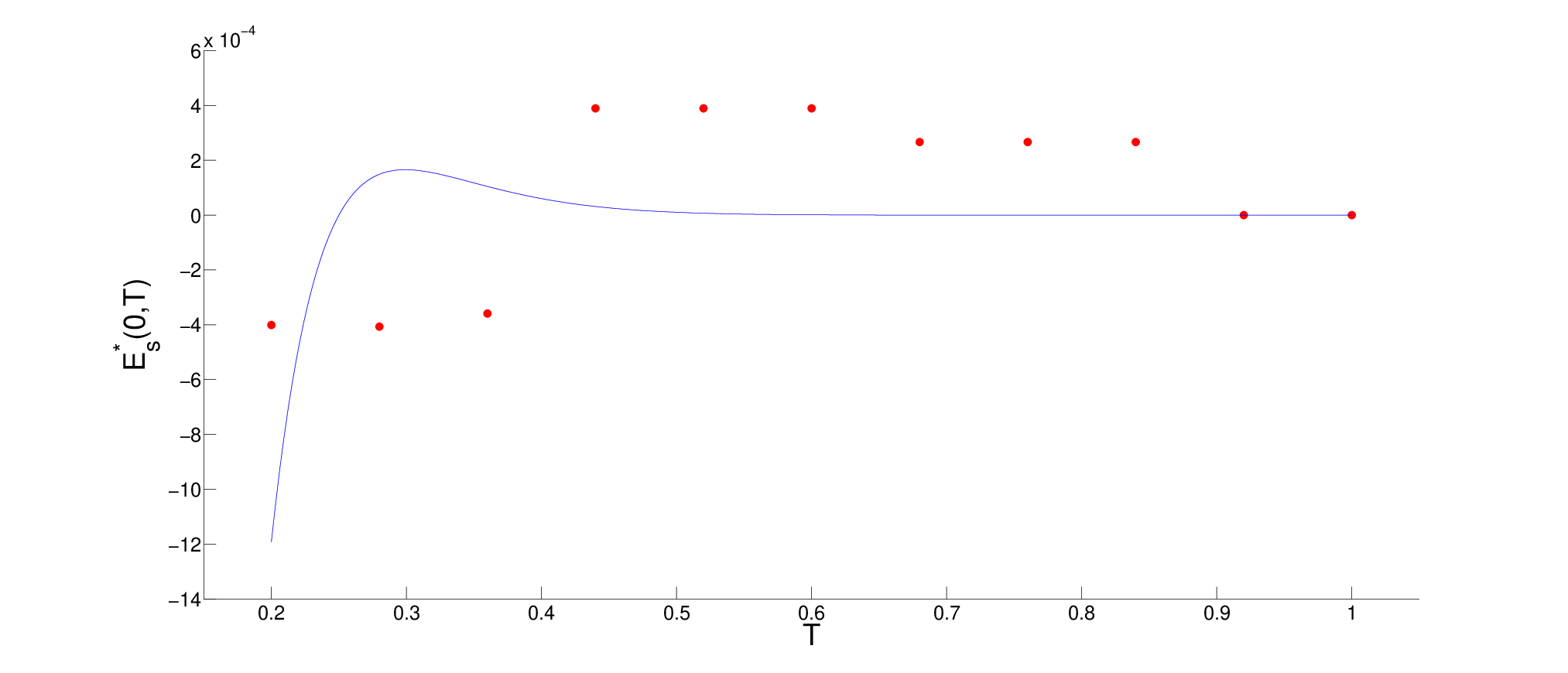
3.2 Time-discontinuous example
Time-periodicity is not a requirement of the theory. In order to push this advantage further than one could legitimately hope, suppose
| (36) |
where is the Heaviside function, and a parameter. This ambitious requirement does not comply with theoretical conditions needed; the bound arising from , and their derivatives in Theorems 2.3 and 2.4 does not exist at some points. Moreover, abrupt switching of locations cannot be achieved in smooth differential equations, and indeed the definition of a stable manifold collapses. How well can the theory be used to help to achieve these computationally?
Choose smooth approximations of (36) given by
| (37) |
Theorem 2.3 gives the requirement and
while applying the shear conditions of Theorem 2.2 as in the previous example locally near gives and
Thus, a control velocity which simultaneously attempts to achieve the required hyperbolic trajectory and tangent vector rotation can be constructed by summing these:
The terms above represent the spikes (associated with the time-derivatives in (36)) needed; these are smooth approximations of Dirac impulses. The system (32) was numerically examined with given by (3.2), with the choice of parameters and . The -discretisation of the previous example was used, with the forward FTLE field computed at each time using the maximum available data (i.e., till ). By evaluating the slopes and intercepts from the extracted ridge, the values of and the -component of were respectively computed at values of . The results, in circles, are compared with the required curves (37) in Fig. 8. There is some error near the abrupt changes, which is inevitable since the FTLE ridges become ambiguous at discontinuities. Nevertheless, the efficacy of the control strategy in this nearly discontinuous situation is remarkable.


4 Concluding remarks
This article approaches the issue of nonautonomous local tangents to stable and unstable manifolds, from two perspectives. First, it hopes to address the finite-time situation in a sense that would appear reasonable with data availability, while retaining the nonautonomous viewpoint within this finite time-range. Under the ansatz of the flow being nearly autonomous, leading-order approximations for hyperbolic trajectories and their attached local stable/unstable manifolds were stated. The relationship between the local tangent vector rotation and the nonautonomous velocity shear was quantified. An attempt to characterise how unknown data from outside a finite-time interval affects flow entities was introduced, by investigating the dependence of an error which depends on the finiteness parameter . The nearly autonomous hypothesis is of course restrictive, and one potential extension would be to assume that the flow is a perturbation of a nearby flow which, while not necessarily autonomous, has its relevant features (hyperbolic trajectory, stable and unstable manifolds) known. This idea was formally used recently [14] for controlling high-dimensional hyperbolic trajectories.
Second, this article addresses the question of controlling the direction of emanation of stable and unstable manifolds from a hyperbolic trajectory. Such local results influence the global stable and unstable manifolds, i.e., the global transport templates, since exponential decay definitions [27, 16, 65] for global invariant manifolds depend on local decay. Standard approaches for defining global stable and unstable manifolds [42, 3] indeed depend on first defining local stable/unstable manifolds, and then obtaining the global manifolds by ‘flowing’ these in time. The local shear velocity required for a given nonautonomous motion of these directions was obtained in Theorem 2.4. The finite-time version of these (see Remark 2.2) simply uses the full data available in the time-range in doing the computation of the shear requirement. The efficacy of this finite-time process was numerically demonstrated using both a time-periodic and a time-discontinuous specification of the tangent vector directions, the latter situation pushing the boundaries of the theorems. To achieve genuinely time-discontinous flow trajectories, impulsive terms are required in the velocities. It has been shown that in the presence of impulsive vector fields one needs to think of stable and unstable pseudo-manifolds which reset themselves at the time instance at which there is an impulse [5, 11]. For the purposes of the numerical verifications of this article, marginally smooth approximations of the discontinuous functions were employed. In both the time-periodic and time-impulsive implementations of the control strategy, excellent performance (as measured by the rotation of FTLE ridges with time) was obtained. Any specified (but small) time-varying reorientation of the stable and unstable manifold directions seems to be possible, providing a tool for controlling the essential skeleton of fluid flows. In particular, by focussing energy on a localised region near the time-varying hyperbolic trajectory, a global transport impact can be achieved. Further analysis and development of these idea, building also on [13, 14, 15], are underway.
Appendix A Proof of Theorem 2.2 (Local manifold directions)
The system (1) is, under the conditions of Hypothesis 2.1, equivalent to
| (47) |
where the higher-order term in uniformly bounded, and . Let be a solution to (47) when such that as ; this solution can be used to parametrise a branch of ’s stable manifold for , for as negative as required. Balasuriya [6, 8] establishes a parametrisation of the perturbed stable manifold in his Theorems 2.7 and 2.8 [6]. These results shall be recast for the present context as
| (48) |
where the superscripts for are for the normal and tangential components respectively. The term of the normal component is expressed in terms of the Melnikov function
| (49) |
It is possible [6] to similarly write the tangential component in terms of a known expression for its -term and a higher-order error term, but as will be seen, this precise expression will not be necessary for this proof. Now, as , , the hyperbolic trajectory, along the stable manifold direction, in each fixed time-slice . Thus, the tangent vector to this, at the point , can be obtained by applying the limit to the -derivative of . This is
| (50) | |||||
where the -subscript represents the partial derivative, and the arguments for and , and the argument for have been suppressed for brevity. Since the limit is required, in this limit
| (51) |
for a constant can be applied; this is since the linearised flow dominates near , and specifically comes in along the stable manifold (tangential to with decay rate ) in this limit. The represents a choice of ‘initial condition’ along the stable manifold, and as will be clear, is inconsequential in the final result. Now, since is a solution to (47) when , and thus
| (52) |
Of the three bracketed terms in (50), the first two are therefore vectors in the direction, whereas the third is in the direction. The second term in the limit behaves according to
It is shown in Lemma B.1 in Appendix B that as , in this limit remains uniformly for . Thus, the error in discarding this term is in the normal direction. The third term of (50) contains the tangential projection and its -derivative, and in this case it will turn out that it is only required to show that this remains . This is easiest accomplished by analysing (48), from which
Since remains uniformly , this asserts the existence of a constant such that . Moreover,
in which the first term remains by the same argument. The second term represents the difference between the tangent vector directions of the perturbed and unperturbed stable manifolds in the limit of approaching the hyperbolic trajectory, and is thus also uniformly by persistence of invariant manifolds [78, 79]. Therefore, the final bracketed term in (50) is bounded by a term , where is independent of .
Collecting all this information together, and substituting the large values into the expression for yields
The rotational angle from towards is and thus equal to to leading-order. This is essentially the slope of the above tangent line in an axis system . Thus,
| (53) |
as , where is uniformly bounded for . The -derivative of (49) is now required in the limit . In this limit, , the sum of ’s eigenvalues at . Putting this along with the other large estimates in (52) into (49) gives the large estimate
When computing , the fact that is a product of with another function of leads to cancellations, and results in
Substituting into (53), putting in , and applying gives (12), where the terms have been combined into one term with bounded for .
Appendix B Proof of normal error term being uniformly
Lemma B.1.
Proof.
For any , define through
| (54) |
Equation (3.1) by Balasuriya [6], developed for the unstable manifold in that case, can be adapted to quantify this. The error required is obtained by replacing the unstable manifold with the stable one, dividing by , and then integating from to . In the present context, this translates to
| (55) |
where
| (56) |
in which the and are locations on the line segment between and arising from Taylor’s theorem applied to and . The uniform boundedness of as is first argued. In this limit, and , with remaining uniformly in . Thus, remains bounded uniformly. Moreover, the hypotheses on and ensure that the and terms are also uniformly bounded in under this limit. Now, applying the large estimates to (55), one gets
| (57) | |||||
In the above, the dominated convergence theorem allowed the limit to be moved into the integral, and s will be used throughout this proof to indicate constants (scalar or vector, dependending on context) independent of . For the proof of Theorem 2.2 as presented in Appendix A, it is not just but its -derivative which needs to be addressed. From (55),
Now, the -derivative of remains bounded uniformly as since and are uniformly bounded by hypothesis. Therefore the second integral above is uniformly bounded by exactly the same argument already made for the (undifferentiated) . In the first integral for large , the fact that the term whose derivative is to be taken collapses to has already been established in (57). Thus, that integral contibutes zero. This establishes that the component of in the normal direction is uniformly for , thereby completing the proof of Lemma B.1. ∎
Acknowledgements: Support from Australian Research Council grant FT130100484, conversations with Gary Froyland, and critical feedback from an anonymous referee, are gratefully acknowledged.
References
- [1] M. Allshouse and T. Peacock. refining finite-time Lyapunov ridges and the challenges of classifying them. Chaos, 25:987410, 2015.
- [2] M. Allshouse and J.-L. Thiffeault. Detecting coherent structures using braids. Phys. D., 241:95–105, 2012.
- [3] D.K. Arrowsmith and C.M. Place. An Introduction to Dynamical Systems. University of Cambridge Press, Cambridge, 1990.
- [4] S. Balasuriya. Direct chaotic flux quantification in perturbed planar flows: general time-periodicity. SIAM J. Appl. Dyn. Sys., 4:282–311, 2005.
- [5] S. Balasuriya. Cross-separatrix flux in time-aperiodic and time-impulsive flows. Nonlinearity, 19:2775–2795, 2006.
- [6] S. Balasuriya. A tangential displacement theory for locating perturbed saddles and their manifolds. SIAM J. Appl. Dyn. Sys., 10:1100–1126, 2011.
- [7] S. Balasuriya. Explicit invariant manifolds and specialised trajectories in a class of unsteady flows. Phys. Fluids, 24:12710, 2012.
- [8] S Balasuriya. Nonautonomous flows as open dynamical systems: characterising escape rates and time-varying boundaries. In W. Bahsoun, G. Froyland, and C. Bose, editors, Ergodic Theory, Open Dynamics and Coherent Structures, volume 70 of Springer Proceedings in Mathematics and Statistics, chapter 1, pages 1–30. Springer, 2014.
- [9] S. Balasuriya. Dynamical systems techniques for enhancing microfluidic mixing. J. Micromech. Microeng., page in press, 2015.
- [10] S. Balasuriya. Quantifying transport within a two-cell microdroplet induced by circular and sharp channel bends. Phys. Fluids, 27:052005, 2015.
- [11] S. Balasuriya. Impulsive perturbations to differential equations: stable/unstable pseudo-manifolds, heteroclinic connections, and flux. page submitted, 2016.
- [12] S. Balasuriya, G. Froyland, and N. Santitissadeekorn. Absolute flux optimising curves of flows on a surface. J. Math. Anal. Appl., 409:119–139, 2014.
- [13] S. Balasuriya and K. Padberg-Gehle. Controlling the unsteady analogue of saddle stagnation points. SIAM J. Appl. Math., 73:1038–1057, 2013.
- [14] S. Balasuriya and K. Padberg-Gehle. Accurate control of hyperbolic trajectories in any dimension. Phys. Rev. E, 90:032903, 2014.
- [15] S. Balasuriya and K. Padberg-Gehle. Nonautonomous control of stable and unstable manifolds in two-dimensional flows. Phys. D, 276:48–60, 2014.
- [16] F. Battelli and C. Lazzari. Exponential dichotomies, heteroclinic orbits and Melnikov functions. J. Differential Equations, 86:342–366, 1990.
- [17] A. Berger, T. Doan, and S. Siegmund. A definition of spectrum for differential equations on finite time. J. Differential Equations, 246:1098–1118, 2009.
- [18] D. Blazevski and R. de la Llave. Time-dependent scattering theory for ODEs and applications to reaction dynamics. J. Phys. A: Math. Theor., 44:195101, 2011.
- [19] D. Blazevski and J. Franklin. Using scaterring theory to compute invariant manifolds and numerical results for the laser-driven Hénon-Heiles system. Chaos, 22:043138, 2012.
- [20] D. Blazevski and G. Haller. Hyperbolic and elliptic transport barriers in three-dimensional unsteady flows. Phys. D, 273:46–62, 2014.
- [21] M. Branicki and S. Wiggins. An adaptive method for computing invariant manifolds in non-autonomous, three-dimensional dynamical systems. Phys. D, 238:1625–1657, 2009.
- [22] M. Branicki and S. Wiggins. Finite-time Lagrangian transport analysis: stable and unstable manifolds of hyperbolic trajectories and finite-time Lyapunov exponents. Nonlin. Proc. Geophys., 17:1–36, 2010.
- [23] M. Budis̆ić and I. Mezić. Geometry of ergodic quotient reveals coherent structures in flows. Phys. D, 241:1255–1269, 2012.
- [24] M. Budis̆ić and J.-L. Thiffeault. Finite-time braiding exponents. Chaos, 25:087407, 2015.
- [25] S. Chandrasekhar. Hydrodynamics and Hydrodynamic Stability. Dover, New York, 1961.
- [26] A. Chian, E. Rempel, G. Aulanier, B. Schmeister, S. Shadden, B. Welsch, and A. Yeates. Detection of coherent structures in turbulent photospheric flows. Astrophys. J., 786:51, 2014.
- [27] W. A. Coppel. Dichotomies in Stability Theory. Number 629 in Lecture Notes Math. Springer-Verlag, Berlin, 1978.
- [28] T. Doan, D. Karrasch, N. Yet, and S. Siegmund. A unified approach to finite-time hyperbolicity which extends finite-time Lyapunov exponents. J. Differential Equations, 252:5535–5554, 2012.
- [29] F. d’Ovidio, V. Fernández, E. Hernández-Garcia, and C. López. Mixing structure in the Mediterranean sea from finite-size Lyapunov exponents. Geophys. Res. Lett., 31:L17203, 2004.
- [30] L. Duc and S. Siegmund. Existence of finite-time hyperbolic trajectories for planar Hamiltonian flows. J. Dyn. Differential Equations, 23:475–494, 2011.
- [31] M. Farazmand and G. Haller. Attracting and repelling Lagrangian coherent structures from a single computation. Chaos, 15:023101, 2013.
- [32] A. Fortin, T. Briffard, and A. Garon. A more efficient anisotropic mesh adaptation for the computation of Lagrangian Coherent Structures. J. Computational Phys., 285:100–110, 2015.
- [33] G. Froyland. An analytic framework for identifying finite-time coherent sets in time-dependent dynamical systems. Phys. D, 250:1–19, 2013.
- [34] G. Froyland, S. Lloyd, and A. Quas. Coherent structures and isolated spectrum for Perron–Frobenius cocycles. Ergod. Th. & Dynam. Sys., 30:729–756, 2010.
- [35] G. Froyland and K. Padberg. Almost invariant sets and invariant manifolds: connecting probablistic and geometric descriptions of coherent structures in flows. Phys. D, 238:1507–1523, 2009.
- [36] G. Froyland and K. Padberg-Gehle. Almost-invariant and finite-time coherent sets: directionality, duration, and diffusion. In W. Bahsoun, C. Bose, and G. Froyland, editors, Ergodic Theory, Open Dynamics, and Coherent Structures, pages 171–216. Springer, 2014.
- [37] G. Froyland, N. Santitissadeekorn, and A. Monahan. Transport in time-dependent dynamical systems: Finite-time coherent sets. Chaos, 20:043116, 2010.
- [38] L. Gaultier, B. Djath, J. Verron, J.-M. Brankart, P. Brasseur, and A. Melet. Inversion of submesoscale patterns from a high-resolution Solomon Sea model: feasibility assessment. J. Geophys. Res. Oceans, 119:4520–4541, 2014.
- [39] F. Ginelli, H. Chaté, R. Livi, and A. Politi. Covariant Lyapunov vectors. J. Phys. A: Math. Theor., 46:254005, 2013.
- [40] M. Green, C. Rowley, and A. Smits. The unsteady three-dimensional wake produced by a trapezoidal panel. J. Fluid Mech., 685:117–145, 2011.
- [41] J. Guckenheimer. From data to dynamical systems. Nonlinearity, 27:R41–R50, 2014.
- [42] J. Guckenheimer and P. Holmes. Nonlinear Oscillations, Dynamical Systems and Bifurcations of Vector Fields. Springer, New York, 1983.
- [43] J. Hale. Integral manifolds of perturbed differential systems. Annals Math., 73:496–531, 1961.
- [44] G. Haller. A variational theory for Lagrangian coherent structures. Phys. D, 240:574–598, 2011.
- [45] G. Haller. Lagrangian Coherent Structures. Annu. Rev. Fluid Mech., 47:137–162, 2015.
- [46] G. Haller and F. Beron-Vera. Geodesic theory for transport barriers in two-dimensional flows. Phys. D, 241:1680–1702, 2012.
- [47] G. Haller and A.C. Poje. Finite time transport in aperiodic flows. Phys. D, 119:352–380, 1998.
- [48] G. Haller and G.-C. Yuan. Lagrangian coherent structures and mixing in two-dimensional turbulence. Phys. D, 147:352–370, 2000.
- [49] D. Karrasch. Linearization of hyperbolic finite-time processes. J. Differential Equations, 254:254–282, 2013.
- [50] D. Karrasch, M. Farazmand, and G. Haller. Attraction-based computation of hyperbolic Lagrangian Coherent Structures. J. Computational Dyn., 2:83–93, 2015.
- [51] D. Karrasch and G. Haller. Do Finite-Size Lyapunov Exponents detect coherent structures? Chaos, 23:043126, 2013.
- [52] D. Kelley, M. Allshouse, and N. Ouellette. Lagrangian coherent structures separate dynamically distinct regions in fluid flow. Phys. Rev. E, 88:013017, 2013.
- [53] J. Lamb, M. Rasmussen, and C. Rodrigues. Topological bifurcations of minimal invariant sets for set-valued dynamical systems. Proc. Amer. Math. Soc., page in press, 2015.
- [54] C. Liang, G. Liao, and W. Sun. A note on approximating properties of the Oseledets splitting. Proc. Amer. Math. Soc., 142:3825–3838, 2014.
- [55] T. Ma and E. Bollt. Differential geometry perspective of shape coherence and curvature evolution by finite-time nonhyperbolic splitting. SIAM J. Appl. Dyn. Sys., 13:1106–1136, 2014.
- [56] A.M. Mancho, D. Small, S. Wiggins, and K. Ide. Computation of stable and unstable manifolds of hyperbolic trajectories in two-dimensional, aperiodically time-dependent vector fields. Phys. D, 182:188–222, 2003.
- [57] A.M. Mancho, S. Wiggins, J. Curbelo, and C. Mendoza. Lagrangian descriptors: A method for revealing phase space structures of general time dependent dynamical systems. Commun. Nonlin. Sci. Numer. Simu., 18:3530–3557, 2013.
- [58] I. Mezić, S. Loire, V. Fonoberov, and P. Hogan. A new mixing diagnostic and Gulf oil spill movement. Science, 330:486–489, 2010.
- [59] P.D. Miller, C.K.R.T. Jones, A.M. Rogerson, and L.J. Pratt. Quantifying transport in numerically generated velocity fields. Phys. D, 110:105–122, 1997.
- [60] B.A. Mosovsky and J.D. Meiss. Transport in transitory dynamical systems. SIAM J. Appl. Dyn. Sys., 10:35–65, 2011.
- [61] D. Nelson and G. Jacobs. DG-FTLE:Lagrangian Coherent Structures with high-order discontinuous Galerkin methods. J. Computational Phys., 295:65–86, 2015.
- [62] K.-D. Nguyen Thu Lam and J. Kurchan. Stochastic perturbation of integrable systems: A window to weakly chaotic systems. J. Stat. Phys., 156:619–646, 2014.
- [63] G. Norgard and P.-T. Bremer. Second derivative ridges are straight lines and the implications for computing Lagrangian coherent structures. Phys. D, 241:1475–1476, 2012.
- [64] V. Oseledets. Multiplicative ergodic theorem: Characteristic Lyapunov exponents of dynamical systems. Trudy MMO, 19:179–210, 1968.
- [65] K.J. Palmer. Exponential dichotomies and transversal homoclinic points. J. Differ. Equations, 55:225–256, 1984.
- [66] T. Peacock and J. Dabiri. Introduction to focus issue: Lagrangian Coherent Structures. Chaos, 20:017501, 2010.
- [67] T. Peacock and G. Haller. Lagrangian coherent structures: the hidden skeleton of fluid flow. Phys. Today, 66:41–47, 2013.
- [68] A. Poje, G. Haller, and I. Mezić. The geometry and statistics of mixing in aperiodic flows. Phys. Fluids, 11:2963–2968, 1999.
- [69] B. Sandstede, S. Balasuriya, C.K.R.T. Jones, and P.D. Miller. Melnikov theory for finite-time vector fields. Nonlinearity, 13:1357–1377, 2000.
- [70] B. Schindler, R. Peikert, R. Fuchs, and H. Theisl. Ridge concepts for the visualization of Lagrangian coherent structures. In R. Peikert, H. Hauser, H. Carr, and R. Fuchs, editors, Topological methods in data analysis amd visualization II, pages 221–236. Springer, 2012.
- [71] S.C. Shadden, F. Lekien, and J.E. Marsden. Definition and properties of Lagrangian coherent structures from finite-time Lyapunov exponents in two-dimensional aperiodic flows. Phys. D, 212:271–304, 2005.
- [72] A. Stroock, S. Dertinger, A. Adjari, I. Mezić, H. Stone, and G. Whitesides. Chaotic mixer for microchannels. Science, 295:647–651, 2002.
- [73] G. Taylor and A. Green. Mechanism for the production of small eddies from larger ones. Proc. R. Soc. Lond. A, 158:499–521, 1937.
- [74] H. Teramoto, G. Haller, and T. Komatsuzaki. Detecting invariant manifolds as stationary LCSs in autonomous dynamical systems. Chaos, 23:043107, 2013.
- [75] G. Wang, F. Yang, and W. Zhao. There can be turbulence in microfluidics at low Reynolds number. Lab Chip, 14:1452–1458, 2014.
- [76] G. Whitesides. The origins and the future of microfluidics. Nature, 442:368–373, 2006.
- [77] K. Yagasaki. Invariant manifolds and control of hyperbolic trajectories on infinite- or finite-time intervals. Dynamical Systems, 23:309–331, 2008.
- [78] Y. Yi. A generalized integral manifold theorem. J. Differential Equations, 102:153–187, 1993.
- [79] Y. Yi. Stability of integral manifold and orbital attraction of quasi-periodic motion. J. Differential Equations, 103:278–322, 1993.