A new and trivial CP symmetry for extended flavor
Abstract
The combination of - exchange together with CP conjugation in the neutrino sector (known as symmetry or -reflection) is known to predict the viable pattern: , maximal Dirac CP phase and trivial Majorana phases. We implement such a CP symmetry as a new CP symmetry in theories with flavor. The implementation in a complete renormalizable model leads to a new form for the neutrino mass matrix that leads to further predictions: normal hierarchical spectrum with lightest mass and () of only few meV, and either or has opposite CP parity. An approximate symmetry arises naturally and controls the flavor structure of the model. The light neutrino masses are generated by the extended seesaw mechanism with 6 right-handed neutrinos (RHNs). The requirement of negligible one-loop corrections to light neutrino masses, validity of the extended seesaw approximation and not too long-lived BSM states to comply with BBN essentially restricts the parameters of the model to a small region: three relatively light right-handed neutrinos at the GeV-scale, heavier neutrinos at the electroweak scale and Yukawa couplings smaller than the electron Yukawa. Such a small Yukawa couplings render these RHNs unobservable in terrestrial experiments.
I Introduction
The discovery of nonzero in 2012 [1] prompted the neutrino physics community to one of its next experimental goals: measure or discard CP violation in the leptonic sector [2]. As one more parameter in the standard three neutrino paradigm joined the list of known quantities, we are only left with three unknowns in case neutrinos are Majorana: neutrino mass ordering, absolute neutrino mass scale and CP violation in the leptonic sector. The last unknown has three sources: one Dirac CP phase analogous to the CKM phase for quarks and two Majorana phases.
From a theory viewpoint, many symmetries were sought over the years in order to predict the CP violating phases of the leptonic sector. The simplest of them that leads to CP violation and viable mixing angles is known as -reflection or which consists on - flavor exchange together with CP conjugation [3]. Often, such a CP symmetry is considered in conjunction with nonabelian discrete symmetries [4, 5, 6, 7]. In fact, many studies were devoted to the definition of CP symmetry in that context [5, 6, 7]. However, differently from many simple flavor symmetries that predicted vanishing , the symmetry allows nonzero but predicts all the presently unknown CP phases: the Dirac CP phase is maximal while the Majorana phases are trivial [3, 8]. Moreover, is also predicted to be maximal, the neutrinoless double beta decay effective mass is restricted to narrower bands and, in simple implementations, leptogenesis is only allowed to occur in the intermediate range of where flavor effects are important [8]. From current global fits [9, 10], we know in fact there is a slight preference for negative and is still allowed.
Two directions were recently pursued to generalize the idea of symmetry. Firstly, we have shown in Ref. [8] that a minimal setting that allowed distinct symmetries in the charged lepton and neutrino sectors consisted of only one abelian symmetry (the combination of lepton flavors or subgroup) and CP symmetry (). This setting was shown to be free from the vev alignment problem that plagues many flavor symmetry models for leptons. In contrast, in Ref. [11], it was shown that maximal and (the prediction for Majorana phases is lost) could follow from much more general assumptions without the imposition of CP symmetry. The necessary conditions involve the symmetry of the charged lepton sector ( to be represented by real matrices in the flavor space and, in the same basis, needs to be diagonalizable by a real matrix. The crucial aspect is the former, which presumably follows from a real flavor symmetry conserved in the charged lepton sector. The neutrino sector cannot be invariant by the same residual symmetry and hence must have a large breaking in the form of misaligned vevs.
Here we try to embed a subgroup of into a discrete nonabelian flavor group in order to increase predictivity but, at the same time, retain the successful features of Ref. [8]. We choose the group which is an extensively studied flavor group (see [12] and references therein). In fact, the first symmetric neutrino mass matrix was obtained with this group [13]. More recent studies involving and CP can be seen in Refs. [14, 15].
We anticipate that the light neutrino mass matrix in our model will have the form
| (1) |
where are real parameters and can be chosen; as usual. This mass matrix is symmetric [3] but has 4 real parameters to describe 5 observables: . Hence, we will have one prediction.
The paper is organized as follows: In Sec. II we describe the new CP symmetry that can be implemented for theories with symmetry. Section III shows that the mass matrix (1) can fit the present oscillation parameters and additionally give predictions for the absolute neutrino mass and CP parities. A complete renormalizable model is shown in Sec. IV where the light neutrino masses are generated by the extended seesaw (ESS) mechanism [16] with relatively light right-handed neutrinos in its spectrum. The approximate symmetry is presented in Sec. V and shown to constrain the flavor structure of the model. Section VI analyzes the constraints on the model coming from (i) the radiative stability of the tree-level result, (ii) validity of the ESS approximation to fit the light neutrino masses and (iii) sufficiently short-lived BSM states that not spoil Big Bang nucleosinthesis. More phenomenological constraints on the presence of relatively light right-handed neutrinos are analyzed in Sec. VII. The conclusions are shown in Sec. VIII and the appendices contain auxiliary material.
II Another GCP for
The group has one three-dimensional irreducible representation (irrep) and three one-dimensional irreps , where the latter is the trivial invariant (singlet). The faithful can be generated by
| (2) |
where generates one of the subgroups and generates the subgroup. Only acts nontrivially on the singlets as
| (3) |
where .
For generic settings where generic irreps of (e.g. a and one charged ) are considered in a model, there is only one possible CP symmetry that can be imposed on the model [6, 7]. As first considered in Ref. [4],11 1 For the triplet only, in the context of the invariant 3HDM, it was first considered in Ref. [17] (erratum) as an accidental symmetry and in Ref. [18] in the course of symmetry classification. CP acts on the representations of (2) and (3) as
| (4) |
where can be chosen as exchange:
| (5) |
The complex conjugation denotes the CP transformation operation on the fields which should be adjoined with the appropriate Lorentz factors for e.g. spin 1/2 fermions. We denote the whole flavor group considering as and it gives rise to a group isomorphic to , denoted as in [4]. Obviously any composition of with an element of is also a GCP symmetry, so any of the 12 GCP symmetries can be chosen as a residual symmetry [15].
In nongeneric settings where only a specific set of irreps is considered, it is clear that there is one more inequivalent option. If only is considered, we can use the usual CP transformation 22 2 It is important to note that the GCP (4), with symmetric , can also be cast in the form (6) by basis change, after which the representation (2) changes and is no longer manifestly real.:
| (6) |
Given that the representation (2) is real, the whole group including will be denoted as where is generated by , which commutes with ( is real).
Now the question is: What is the transformation law for the other irreps (if any is consistent)? We can deduce them by noting that the transformation (6) acts on the representation (2) trivially, i.e.,
| (7) |
if we apply on any , in this order, , the transformation or and then . In contrast, for , the same set of operations induces
| (8) |
Here we are identifying with its three-dimensional irrep in (2). Given that (8) and (7) lead to different rules (map different conjugacy classes), they cannot be equivalent. These mapping rules in the group are called automorphisms and only (8) and (7) are nonequivalent for . So these are the only possibilities for defining GCP in the presence of symmetry [6].’
We can now deduce that one transformation law for the singlets that is compatible with (6) and (7) is the trivial transformation
| (9) |
However, this transformation law can only be used if the complex field is neutral under any other group, including the Lorentz group, i.e., it must be a scalar 33 3 One could also use (9) as charge conjugation for a pair of Majorana fermion fields where acts by rotation in the plane. . In this case, we can split any complex scalar into its real and imaginary parts, , and consider the action of of as a rotation in the plane of , hence a real representation that is trivial under , i.e., , are CP-even real scalar fields.
On the other hand, if carries other complex quantum numbers (it excludes ) other than , say a charge of , then (9) is not compatible with the fact that CP should reverse the charge . Therefore, in this case another field with the same charge (or any other quantum number) needs to be introduced to define the transformation
| (10) |
so that both sides transform as by but the field of charge is mapped to a field of charge . This is also the transformation law for fermions. To summarize, the irreps and are exchanged by ,
| (11) |
unless can be identified with . Therefore, for charged fields (such as the SM fields or any chiral fermion) the irreps need to be introduced in pairs. It is always possible to recast (11) as the usual CP transformation by changing basis; see appendix B of Ref. [8] for the explicit basis change.
Compatibility with the triplet transformation law (6) can also be checked independently by forming an invariant with two triplets (say fermionic and left chiral) and a scalar , and ensuring that maps an invariant to an invariant [6]. The only trilinear invariant involving and is
| (12) |
It is tranformed by (6) (for ) and (9) (for ) to
| (13) |
which remains as an invariant.
The symmetry (associated to the trivial automorphism) can be straightforwardly extended for other groups with structure such as the family [e.g. [19]] or some of its subgroups such as or . The only difference is that the triplet representations would be complex and CP symmetry would act as usual.
We stress that the symmetry for has not been considered for flavor model building before. This possibility is raised in the general context of discrete nonabelian symmetries in [6] but no model application was discussed. For , this possibility was mentioned in [15] but it was not pursued. Ref. [7] discards this kind of CP symmetry dubbing it as CP-like symmetries but—as we will see for the simple case of —no theoretical consideration prevents its use. As an added bonus, we will see that the transformation property (9) allows us to avoid the vev alignment problem [8].
III Mass matrix
We first analyze our mass matrix (1) in the flavor basis to show that we can correctly fit the oscillation parameters. This is a new form for the neutrino mass matrix that has not been considered so far.
The symmetry of (1) implies that and are automatic [3] and the diagonalization
| (14) |
can be performed by a matrix of the form
| (15) |
with conventionally real and positive. The Majorana phases are trivial and possible CP parities appear along with the eigenvalues , . We denote the different cases of CP parities by the sign of as
| (16) |
In addition to being symmetric, the mass matrix in (1) obeys
| (17) | ||||
Thus cyclic permutation of leaves all observables of invariant while a transposition () flips the Dirac CP phase: . Hence, permutations of solutions for are solutions as well.
III.1 Obtaining the masses
To extract the light neutrino masses, it is more convenient to change to a real basis:
| (18) |
where
| (19) |
Now is real symmetric and can be diagonalized by a real orthogonal matrix.
The eigenvalues of will correspond to the light neutrino masses with its CP parities. They are solutions of the characteristic equation
| (20) |
with coefficients
| (21) | ||||
It is clear that is a special point where
| (22) |
is a solution; permutation of still leads to a solution. However, our mass matrix (1) with and with the second and third columns (rows) exchanged is invariant by cyclic permutations which means it is diagonalized by . This mixing matrix is clearly in contradiction with experiments, a fact that still applies if (for hierarchical ). Hence, we need to analyze the cases away from .
Generically we can invert (21) and obtain as functions of and . A simplification is achieved for generic by defining
| (23) |
Then the equations in (21) can be rewritten as
| (24) | ||||
where
| (25) |
The key relation that can be extracted from (24) is that should now be roots of the cubic equation similar to (20) but with coefficients modified by
| (26) |
This construction gives as functions of and , except for permutations of . The solutions (22) for are modified as differ from unity when . Moving away from , both functions increase monotonically ( reaches asymptotically as ).
Now, the distortions caused by cannot be too large because the need to be real. To illustrate this point, compare the two polynomials
| (27) |
where the second polynomial differs from the first just by a small deviation in the third coefficient. The first polynomial has three real and distinct roots while the second polynomial has only as a real root. This can be confirmed by calculating the discriminant of the factored second-degree polynomials: and for and respectively. We can see that two quasidegenerate eigenvalues are specially sensitive to deviations by . This is the case of IH with CP parities or .
The values for that allow real solutions for can be extracted from the discriminant of the cubic polynomial (20) for which
| (28) |
In Fig. 1 we show the values of as a function of the lightest mass where the discriminant above is non-negative; we use the current best fit values for the mass differences [9]. The figure on the left (right) corresponds to NH (IH) and the various possibilities for CP parities are depicted in different colors. For IH, only the case of CP parities and have wide regions for for a given mass ; the remaining cases only have very narrow ranges of possible , including which is phenomenologically excluded. The other possible narrow range for for IH- (e.g. for ) is also phenomenologically excluded because it leads to and two mixing angles are vanishing.
We also illustrate in Fig. 2 the deviations from when moves away from . varies only in the range where the discriminant (28) is non-negative, as shown in Fig. 1. Note that close to the critical values of () two (or more) tend to be quasidegenerate. This is a generic phenomenon.
III.2 Seeking solutions
After an exhaustive numerical search we conclude that the mass matrix (1) is only compatible with oscillation data for normal hierarchy (NH) and CP parities and . The cases of IH and quasidegenerate masses are excluded. The lightest neutrino mass is restricted to
| (29) | ||||||
The predictions for the contribution for neutrinoless double-beta decay coming from light neutrinos is given by
| (30) | ||||||
They fall inside the regions denoted by NH- and NH- in Ref. [8]. Note that . For future use, we also list
| (31) | ||||||
The parameter distribution for the two sets of solutions is shown in Fig. 3 for as functions of (left), and as a function of (right). The values and are fixed from symmetry and we only consider values for and within 3- of the global fit in Ref. [9] by varying and independently. Approximate values are obtained from the procedure below.

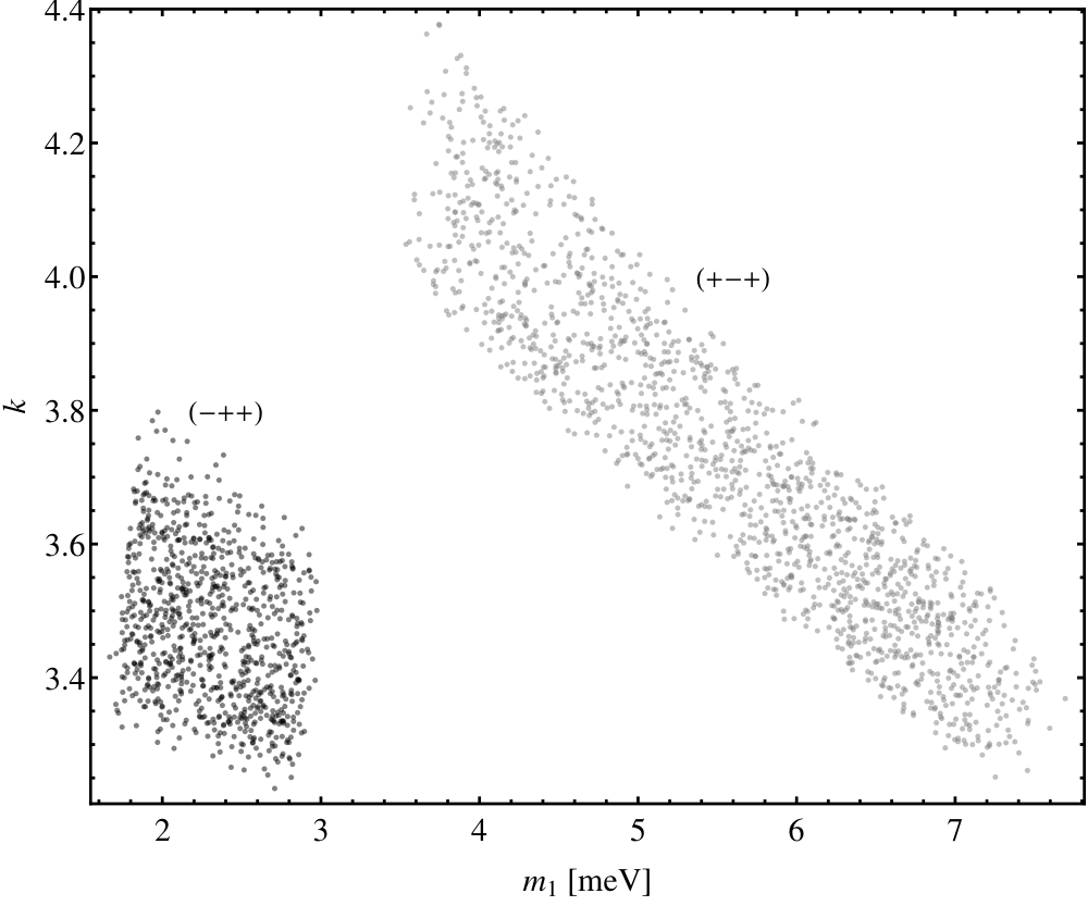
We use the following procedure to exclude solutions and search for approximate solutions:
- 1.
- 2.
Then, we diagonalize (1) to extract the mixing matrix . We adopt the ordering of eigenvectors to satisfy
(32) The ordering of follows. This means that our mass eigenstates are in the order of decreasing contribution to ( contributes the most and so on) and not in a specific mass ordering. This definition explains the color flipping in Fig. 2 for .
- 3.
At last, we check if the mass ordering is correct and if the mixing angles fall inside the 3- ranges. An illustration of this step is shown in Fig. 4.
One remark on this procedure is in order: to correctly fit the oscillation parameters we need that (i) the mixing angles are correct and (ii) the mass ordering is correct. The condition (ii) arises because mass eigenstates are defined by (32) and mass orderings that do not correspond to NH or IH are excluded. For example, we can read from Fig. 4 that the correct values for both and are only achieved for , as can also be confirmed in Fig. 3. Correct values for can also be obtained for but as well as the mass ordering in Fig. 2 is not correct: for , has a greater contribution from the heaviest state ( in red) than the second heaviest state ( in green).
IV Extended seesaw model
Here we present a low-scale seesaw model where the light neutrino mass matrix has the form (1). The model will retain the successful predictions of [8] for the low-energy neutrino observables but additional predictions arise due to the more constrained nature of the group . Two sets of heavy neutrinos – one at the GeV-scale and another at the electroweak scale – arise naturally due to the extended seesaw mechanism (ESS) [16]. The combination of lepton flavor numbers will be approximately conserved in the model.
The flavor symmetry of the model will be (), explained in Sec. II 44 4 Note that the combined group is a direct product because both factors commute [8].. The SM lepton fields are, however, all singlets of and only feel the subgroup 55 5 This contrasts with most of the models for leptons where at least the lepton doublets form triplets [12] , thus entirely avoiding the need of any vev alignment in this sector. An auxiliary will also be necessary in the neutrino sector. The SM lepton fields are assigned to while the Higgs doublet is invariant; are lepton doublets while are the charged lepton singlets. Thus in (11) can be identified with [8]. There are also two sets of SM singlets (right-handed neutrinos) and , , assigned to and respectively. Hence, only the neutrino sector feels the full group through . We also need complex flavons and , and a real . The full assignment can be seen in table 1. Additional fields necessary to break in the charged lepton sector are not shown since they can just be adapted from [8].
The charged lepton sector at the electroweak scale will effectively be the SM one 66 6 For simplicity we are considering the UV completion by heavy leptons but the multi-Higgs version can be equally considered with the difference that the Higgs that couples to the flavors is distinct [8].
| (33) |
where the subgroup is unbroken but is broken at a higher scale by a CP-odd scalar [8] so that the correct splitting for and is generated ().
The neutrino sector at the high scale is given by
| (34) | ||||
where we have defined singlet combinations of two triplets of as
| (35) | ||||
Note that acts as
| (36) | ||||
and and transform like and denotes the usual CP conjugate of the chiral fermion . Therefore, are real and , due to . The parameters can be further chosen real and positive by rephasing and .
The mass matrix for after EWSB will be
| (37) |
where
| (38) | ||||
where
| (39) |
In this model, we are considering that acquire very small vevs which lead to the real Majorana masses for and also
| (40) |
We justify the hierarchy of vevs in appendix B.
Considering that is composed of bare masses, the ESS limit is naturally achieved [16]: and also . We can see that there are two sources of lepton number violation (LNV) in (34) 77 7 If .: (a) large scales and (b) low-scales .
At tree level and leading order we obtain
| (41) | ||||||
with light-heavy mixing
| (42) | ||||
Additional mixings can be seen in appendix A. We can see that the small LNV scale only enters while the large LNV scale contributes only to heavier masses. Given that the mass matrix for the heavier states are approximately unchanged, we can define
| (43) |
assuming positive quantities. The leading correction can be seen in appendix A.
Explicitly, the light neutrino mass matrix is
| (44) |
which has the desired form (1) with
| (45) |
We have used the shorthand ; cf. (38). The fitting of the light neutrino parameters in Fig. 3 implies
| (46) | ||||
Also, the sign change of one of the needs to be generated by and not by which is always positive.
Although the heavier states are frequently chosen to lie above the TeV scale [20, 16], in our case (i) a negligible one-loop contribution for light neutrino masses, (ii) validity of the ESS approximation and (iii) BBN constraints will essentially restrict to the electroweak scale; see Sec. VI and (72) for a benchmark point.
V Approximate limit
We consider first the limit where of is only broken by the small quantities in . This means that below the scale of , is only broken by light neutrino masses. This approximate symmetry corresponds to the lepton flavor triality (LFT) [21] where lepton fields carry the discrete charges
| (47) |
is related to by change of basis .
The heavy vevs of conserve LFT when
| (48) |
This feature is justified in appendix B. In this case, after and in the limit , the Lagrangian (34) is in fact invariant by the continuous version of (47) with charges [8]
| (49) |
It corresponds to the combination of family lepton numbers. The approximate conservation of will lead to a number of consequences.
In this limit the mass matrix (41) and mixing (42) of the heavy neutrinos yield
| (50) | ||||
where the masses read 88 8 We keep using the same name for the heavy neutrino fields although they have a small component of and .
| (51) |
These relations allows us to trade and for physical masses:
| (52) |
The mass matrix is invariant by cyclic permutations and then is an eigenvector. We can diagonalize it by
| (53) |
giving
| (54) |
The matrix was defined in (19). Therefore, is a Majorana fermion of charge 0 and are degenerate Majorana fermions that form a (pseudo-)Dirac pair of fields with charge . The latter implies that LNV effects induced by exchange will vanish in this limit.
The active-sterile - mixing reduces to
| (55) |
It is important to note that in this approximation
| (56) |
and the electron flavor is only coupled to .
VI One-loop contributions and BBN constraints
Now we should compute the one-loop contributions to light neutrino masses. When the lightest heavy RHN mass lies below 100 MeV, the one-loop contributions to can be sizable [22], although such a sterile neutrinos are severely constrained by cosmological data [23]. Heavy neutrinos with electroweak-scale masses can still induce sizable contributions [24, 20] and the dominant (and finite) one comes from light neutrino self-energies with Higgs or exchange [25, 26, 27].
We can write the self-energy contribution as
| (57) |
where the loop function is given by
| (58) |
with and being the and Higgs boson masses, respectively; is the electroweak scale. This contribution should be added to the tree-level contribution (44) coming from the ESS mechanism. We should note that heavy neutrino masses at the electroweak scale leads to a contribution (57) functionally similar to the tree-level contribution , but smaller only by the loop factor [25] [notice ]. Therefore, the one-loop contribution in the ESS mechanism can possibly be large since the cancellation that occurs in the tree-level mass matrix is not expected to carry over to the one-loop contribution.
We can adapt the one-loop contribution for generic type-I seesaw (57) to the extended seesaw with mass matrix (37) as
| (59) |
We have first block diagonalized (see appendix A) and then used the basis where and is diagonal ( and ). It is also possible to write the expression in terms of the light-heavy mixing angles as
| (60) |
We can see that generically the contribution from the heavier states dominates over the contribution from because the smaller mixing angle is compensated by and grows with .
For our purposes, it is useful to define the adimensional function as
| (61) |
A slightly different definition can be seen in [28]. This function peaks at the electroweak scale with maximum and decreases away from the peak with rate slower than for ; see behaviour in Fig. 5. This function allows us to rewrite (59) as
| (62) |
We have used the shorthand and similarly for .
Computing (62) in our model in the symmetric limit, we obtain the texture
| (63) |
whose nonzero entries correspond to . Explicitly,
| (64) | ||||
where . We have used Eqs. (38), (53) and . We note that indeed the one-loop contribution can lead to an unacceptably large contribution. For example, for , the one-loop contribution leads to a few keV. From Fig. 5 we also see that to lower the contributions from (64) to acceptable values by increasing requires very large values of the order of . Therefore, to have TeV-scale (or lower) right-handed neutrinos, we need to lower the scale of or arrange some cancellation between either the various one-loop contributions or between the tree and one-loop ones [27]. We consider this possibility unappealing and do not pursue it any further.
In order to preserve our predictions of Sec. III we confine ourselves to the case where the loop-induced contributions (64) are negligible compared to the tree level ones in (1). To visualize the possible regions in parameter space, we show in Fig. 6 the regions (blue) in the - plane (left) and - plane (right) where the one-loop contribution is at most 10% of the tree-level contribution for the (left) and (right) entries. For definiteness we fix the tree-level values to
| (65) | ||||
These values are in agreement with (30) and (31). We choose to plot the dependence on because the one-loop contributions depend dominantly on (rather than on the lighter ) in the ESS approximation. For example, if we increase the ratios , the blue regions shrinks down only slightly for large . For completeness, we also show the curves for unit ratio (dashed).
The next step is to ensure that the tree-level contribution themselves – as they depend on the model parameters as in (45) – lie in the necessary ranges of (30) and (31) (also Fig. 3). For that purpose, we rewrite the sum of all relations for in (45) as
| (66) |
where . We have also used (52) to eliminate . An analogous relation is valid for the entry:
| (67) |
As in order to satisfy the ESS approximation, we require
| (68) |
These conditions define allowed regions for - and - which are shown as orange regions in Fig. 6. We also show in dashed orange curves the values where the above ratios assume the values (left) and (right). We use the same reference values in (65).
The conclusion is that the overlapping (allowed) regions impose upper bounds on the heavy RHN states:
| (69) |
This constraint puts the RHN states at the GeV-scale. We also note that had we allowed , would be unbounded but restricted to a narrow band for . A similar consideration applies to .
As the last constraint, we note that cannot be pushed to arbitrarily low values because it necessarily makes the lighter BSM states very long-lived 99 9 We assume all the scalars to be heavier than . . In order to not spoil the successful prediction of Big Bang nucleosinthesis (BBN), we require that the lifetimes of all the BSM states do not exceed 0.1 s. It is enough to require that for the lighter states. As their masses lie at the GeV-scale or lower, the main decay modes involve or exchange through active-sterile mixing with decay into light neutrinos, electrons or pions [29]; see appendix C for more details. The allowed regions are shown in green in Fig. 6 where the border is determined by the fixed ratios of (65); the interior refers to (left) or (right) in accordance to the ESS approximation. For completeness, we also show as dashed green curves the points where and (left) or (right).
The combination of all the constraints discussed above, leads to the overlapping regions of Fig. 6. The parameters are restricted to the values listed in Table 2. The restriction means that points outside the overlapping region violate some constraint above for the reference values (65).1010 10 The actual green regions may lie slightly to the left for two reasons: (i) we only include the dominant decay modes for listed in appendix C and (ii) the strict lifetime limit for successful BBN may be slightly relaxed depending on the details of the model at the BBN era [30]. Points inside the overlapping regions need to be further checked for all the constraints as they depend on other parameters not shown in the figures. Moreover, the parameters are not all independent as one ratio is fixed through (46) and
| (70) |
To use tree-level values different from (65) but restricted to (30) and (31), we just need to reread Fig. 6 with the vertical axis relabeled as
| (71) | ||||
This is possible because all the defining relations, Eqs. (64) (66), (67) and the active-sterile mixing in the decay rates (ap. C) depends on or . For the same reason, the blue and orange curves of the right figure of Fig. 6 are identical to the ones on the left if we identify , where is basically the factor .
As an example, the following values pass all the constraints and are also marked in Fig. 6 by crosses:
| (72) | ||||
The intermediate scales and can be obtained from (52). They set a lower bound for the scales and while the masses can be chosen . Using the values in (72) as a benchmark, we plot in Fig. 7 the ratio of the one-loop contribution to the tree-level value of where now we vary and rescale simultaneously by fixing . For the benchmark values (72), the one-loop contribution is indeed less than 10% of the tree-level value. We also show the ratio of the lifetime to the limit of 0.1 s (solid gray) and confirm that needs to be larger than around 1 GeV.
Finally, we can estimate the amount of cancellation that is built-in in our ESS mechanism implementation. Rewriting (66) in the form of the naive seesaw relation,
| (73) |
we extract
| (74) |
if we use Table 2. Analogously, for the entry, we obtain . These values are in agreement with the radiative stability conditions discussed in Ref. [20] that estimated a lower bound of for a GeV-scale right-handed neutrino mass.
VII Other phenomenological constraints and breaking
We analyze here other phenomenological constraints coming from the existence of GeV-scale heavy neutrino with mixing with the light neutrinos at the order of
| (75) | ||||
where we have used (52) and simplified the notation for . For the values (72),
| (76) |
The other mixing angles are either of the same order or vanishing in the limit of conservation; cf. (55). At the same time, the Yukawa couplings to the RHN in our model are even more suppressed,
| (77) | ||||
They are smaller than the electron Yukawa coupling and thus the Higgs couplings to the RHN are very much suppressed (their are smaller than the mixing ). Hence, the main interactions of the RHN to the SM fields occur through active-sterile mixing in (75).
However, it is clear that indirect detection constraints such as lepton universality violation or electroweak precision tests are not able to restrict or probe such a small mixing angles [31, 32]. They are also unobservable through direct detection in meson decays [31, 32, 29] or in colliders [33]. Note that this scenario contrasts with models where Higgsses charged under [or ] may induce large lepton-flavor-violating Higgs decays [34].
For the same reason, lepton flavor violation (LFV) constraints are very weak in our model. The suppression is even larger because LFV processes such as or are forbidden in the limit of conservation. One can also see this in (55) as always vanish. Being a larger group, is more constraining than lepton flavor triality [21] and the former only allows . However, when this process is mediated only by heavy neutrinos, it occurs through box diagrams that are very much suppressed [35]. These conclusions are not modified when breaking effects are considered. See appendix D.
At last, we can analyze the limits coming from neutrinoless double beta decay, which are the strongest involving the mixing with the electron flavor. Since the active-sterile mixings are all vanishing or of the same order in the symmetry limit, cf. (55), we expect that this process will pose the strongest constraint on the mixings.
The half-life of the process is proportional to [31, 20]
| (78) |
where quantifies the effective momentum transfer inside the nucleus and represent the masses of the additional heavy neutrino states that mix with the three active ones. The light neutrino contribution depends on
| (79) |
with contributions arising from tree and loop contributions
| (80) |
For symmetric theories, it is confined to bands depending on the CP parities of the light neutrinos [8]. For a review on generic aspects of see Ref. [36]. We are assuming we are confined to the parameter space where the one-loop contributions are negligible compared to the tree-level one.
Considering (78), we can define, in analogy to the light neutrino contribution [22],
| (81) |
where (corresponding to in Ref. [27]) and we have already specialized to . We disregard the subdominant contribution from the heavier states . If the heavy neutrino masses are much larger than the typical momentum transfer in the nucleus, , we can approximate
| (82) |
Taking the GERDA+Helderberg-Moscow limit, at 90% C.L. [37], it translates into
| (83) |
We can see that the contribution from light neutrinos predicted in our model (30) is at least two orders of magnitude smaller than the limit above. It remains to be checked if the contribution from exchange can give a larger contribution.
In the limit where (or LFT) in (49) is conserved, only couples to the flavor and thus to ; cf. (56). We can then write
| (84) |
where we have assumed that . For the values (72), this contribution is negligible. One could lower the mass to increase this contribution (including the correction in (81)) but it hits the BBN constraint rather quickly. Such a feature is illustrated in Fig. 7 where the ratio of the contribution from exchange to the limit of 0.3 eV is shown in dashed green. Note that we use the expression (81) to account for . We can see that the is negligible for larger than 1.33 GeV. Even if we allow the lifetime of to be around 1 s, it will still be unobservable in future experiments. It is possible, however, that for and much larger than the light neutrino contribution.
VIII Conclusions
We have presented a new CP symmetry applicable to models with flavor symmetry and other groups with the structure such as . To implement this type of CP symmetry, the singlets that are fermions or carry other quantum numbers should appear in pair with another with the remaining quantum numbers identical to those of . This new CP symmetry allows us to avoid the vev alignment problem in close analogy to the construction using and symmetries [8]. This feature partly follows because the SM lepton fields are singlets of and only feel the subgroup which is contained in .
We have constructed an explicit renormalizable model that leads to a new form for the light neutrino mass matrix, cf. (1). It retains the successful predictions of – namely maximal , maximal Dirac CP phase and trivial Majorana phases – but because of the structure it also predicts normal hierarchy with the lightest neutrino of only few meV; see (29). The CP parities are also restricted to two possibilities which effectively fix the effective parameter contributing to neutrinoless double beta decay.
The model itself is based on the extended seesaw mechanism which naturally leads to relatively light right-handed neutrinos and heavier . After enforcing negligible one-loop contributions to light neutrino masses, ensure the ESS approximation and require fast enough decay rate of the BSM states to avoid BBN constraints we only find a small allowed region in the parameter space: neutrinos lie at the electroweak scale and the lighter lie at the GeV scale; see Fig. 6. To suppress the one-loop contributions, it is required that their Yukawa interactions with the SM fields should be smaller than the electron Yukawa coupling. Consequently the active-sterile mixing is largely suppressed, rendering the right-handed neutrinos practically unobservable in terrestrial experiments.
The flavor structure of the model is largely determined by the approximate conservation of the combination of lepton flavors, which suppresses various flavor changing processes such as . Moreover, only mixes appreciably to and the mixing of to the flavors are of the same order of magnitude.
Acknowledgements.
The author would like to thank the Maryland Center for Fundamental Physics of the University of Maryland at College Park, USA, for the hospitality where this work initiated. The author also thanks Rabindra Mohapatra for discussion on several points. Partial support by Brazilian Fapesp grant 2013/26371-5 and 2013/22079-8 is acknowledged.Appendix A Block diagonalization of
The ESS mechanism naturally leads to two disparate scales for the right-handed neutrinos: the lighter () and the heavier (). So it is useful to write the complete neutrino mass matrix (37) in a basis where is block diagonal:
| (85) |
The mass matrix is given by (41). The subleading correction to is
| (86) |
where indicates the transpose of the previous matrix.
The block diagonalization is performed by
| (87) |
with
| (88) |
Further block diagonalization leads to the results in (41) and (42). The complete diagonalization is performed by
| (89) | ||||
The fields on the left-hand side are in the flavor basis and appear in (34); the ones on the right-hand side are the mass eigenfields and is the PMNS matrix in the flavor basis. We have neglected nonunitary effects and the small mixing angles were already given in Eqs. (42) and (88).
Appendix B Comments on the potential
Here we justify the approximate conservation of that follows from the conserving vevs for in (48).
We start by observing that when the potential for is invariant by global rephasing, the potential is identical to a potential with three Higgs doublets with symmetry and we know that (48) can be exactly a global minimum [38].
The addition of the two independent quartic terms that breaks but conserves ,
| (90) |
can be chosen to maintain such alignment and also to make real and positive. We stress that these and other quartic terms are not invariant by but only the subgroup. These terms also help to maintain the deviations of in the real direction since the coefficients are real because of .
Now we add the interactions of with and . The relevant terms are
| (91) |
and
| (92) |
where can be complex and the singlet combination was defined in (35). Clearly there is no rephasing symmetry for and no Goldstone will be generated.
The mild hierarchy of ESS scales
| (93) |
implies a mild hierarchy between and . We can choose so that . For an order one , the small can be generated from (91) by a vev seesaw analogous to type-II seesaw [39]. In this case is electroweak scale. For a vev seesaw cannot be implemented because vanishes for the minimum (48). But we can always take , adjust the potential parameters to obtain and make in (92) small enough so that (48) is only slightly disturbed. The mass of the lightest physical states of will be around and heavier than . Note that and should be comparable because they lead to .
At last, in principle the new scalars could be produced in Higgs decays through the Higgs portal but the current limits on the invisible Higgs decays are still weak [40] and can be avoided by decreasing the portal interactions.
Appendix C Decay rates for
In our theory the RHN heavy states are the lightest new states beyond the SM which lies at the GeV-scale. The dominant decay channels involve or exchange through mixing with light neutrinos or charged leptons [29]. The decays are highly suppressed.
To ensure that the production of light nuclear elements in the early Universe (Big Bang nucleosinthesis) are not disturbed by the presence of new particles, we require that the lifetimes of the new states are shorter than 0.1 second. In that case these new particles are thermalized much before the BBN era and they decay fast enough. RHNs lighter than around 100 MeV conflict with direct detection constraints and are excluded [30, 41].
Assuming the symmetry, the active-sterile mixing (55) leads to the dominant decay channels [29]
| (94) | ||||
We neglect the decay to other channels. The decay rates for these processes can be taken from Ref. [29]:
| (95) | ||||
In each expression, refers to the mass of the decaying particle and each decay rate contributes twice due to the charge conjugate mode. Moreover, the expression for are identical to the expressions for and note that we can write
| (96) | ||||
We are also assuming that is slightly broken so that are distinct Majorana fermions. In the exact limit, forms a Dirac heavy neutrino with charge unity while its conjugate carries charge . In this case, the decay rates of are the same as without the factor two multiplication (the last one would be doubled due to diagonal mixing).
Appendix D Deviations of
In the fermion sector our model is approximately invariant by , which includes (47) of . In the first approximation considered is only broken in the neutrino sector by small in (37). Identical charges (49) can be assigned to all the lepton fields (49) if we change basis to
| (97) |
We show below the form of the mass matrices in this basis with small breaking.
An additional (and also LFT) breaking effect in the neutrino sector is induced by deviations in from (48), which can be parametrized as
| (98) |
The deviation is quantified by . is expected to be conserved as there is no CP violating interactions for . Hence we expect .
The mass matrices (38) in the basis read
| (99) | ||||
where the breaking parametrization (98) for was used. The explicit change of basis is induced by
| (100) |
Conservation of implies and real . In the mass matrices it implies the usual invariance:
| (101) |
In the same basis, the neutrino mass matrix (50) becomes
| (102) |
where were given in (51) and we have added the superscript (0) to indicate the limit explicitly. A generic deviation respecting arising from can be parametrized by
| (103) |
where , .
The combination is now diagonalized by
| (104) |
where denotes the maximal mixing matrix in (19). One can check that is a real orthogonal matrix given by
| (105) |
The small parameters are combinations of the small quantities in (103) and are defined by
| (106) |
all are real. The primed are rotated as
| (107) |
with angle . One can note that the angle depends only on the deviation parameters and does not need to be small due to the degeneracy . The formula (105) is valid as long as and covers the case where so that the mass splitting for can be substantial:
| (108) | ||||
We are adopting .
Putting all together we find the deviation from (55):
| (109) | ||||
where are small parameters that depend on the small parameters while are order one, approximately unitary, quantities. The deviation from maximal (23) mixing in (55) can be large due to mass degeneracy in the limit. Again the superscript denotes the limit. Note that has the structure
| (110) |
Considering the deviation (109) in mixing, we can include the effects of exchange in as
| (111) |
where are now nondegenerate and include the breaking effects. It is clear that the contribution of () exchange can be comparable to exchange only if
| (112) |
This cannot happen in our theory.
We can also confirm that breaking is not enough to induce observable lepton flavor violating processes such as . The vanishing rate is now proportional to the breaking effects. Considering only in the loop, the branching ratio yields [24]
| (113) |
where and is defined in Ref. [24]. For example, . Therefore, the predicted rate is much below the current MEG limit [42] and there is no constraint even if is as large as 1%. One can also check that contributions lead to similar results. Future conversion experiments in nuclei [43] can improve the limit by few orders of magnitude but our model predictions are still suppressed. Hence, LFV processes constraints are much weaker than in our model.
References
- [1] K. Abe et al.[T2K collaboration], Phys. Rev. Lett. 107 (2011) 041801 [1106.2822]; P. Adamson et al. [MINOS Collaboration], Phys. Rev. Lett. 107, 181802 (2011) [1108.0015]; Y. Abe et al. [DOUBLE-CHOOZ Collaboration], Phys. Rev. Lett. 108, 131801 (2012) [1112.6353]; F. P. An et al. [DAYA-BAY Collaboration], Phys. Rev. Lett. 108, 171803 (2012) [1203.1669]; J. K. Ahn et al. [RENO Collaboration], Phys. Rev. Lett. 108, 191802 (2012) [1204.0626].
- [2] A. de Gouvea et al. [Intensity Frontier Neutrino Working Group Collaboration], 1310.4340 [hep-ex].
- [3] P. F. Harrison and W. G. Scott, Phys. Lett. B 547, 219 (2002) [hep-ph/0210197]; W. Grimus and L. Lavoura, Phys. Lett. B 579, 113 (2004) [hep-ph/0305309]; Fortsch. Phys. 61, 535 (2013) [1207.1678].
- [4] R. N. Mohapatra and C. C. Nishi, Phys. Rev. D 86, 073007 (2012) [1208.2875];
- [5] F. Feruglio, C. Hagedorn and R. Ziegler, JHEP 1307, 027 (2013) [1211.5560];
- [6] M. Holthausen, M. Lindner and M. A. Schmidt, JHEP 1304 (2013) 122 [1211.6953];
- [7] M. C. Chen, M. Fallbacher, K. T. Mahanthappa, M. Ratz and A. Trautner, Nucl. Phys. B 883 (2014) 267 [1402.0507];
- [8] R. N. Mohapatra and C. C. Nishi, JHEP 1508 (2015) 092 [1506.06788 [hep-ph]].
- [9] M. C. Gonzalez-Garcia, M. Maltoni and T. Schwetz, JHEP 1411 (2014) 052 [1409.5439].
- [10] G. L. Fogli, E. Lisi, A. Marrone, D. Montanino, A. Palazzo and A. M. Rotunno, Phys. Rev. D 86 (2012) 013012 [1205.5254 [hep-ph]]; D. V. Forero, M. Tortola and J. W. F. Valle, Phys. Rev. D 86 (2012) 073012 [1205.4018 [hep-ph]].
- [11] H. J. He, W. Rodejohann and X. J. Xu, Phys. Lett. B 751 (2015) 586 [1507.03541 [hep-ph]]; A. S. Joshipura and K. M. Patel, Phys. Lett. B 749 (2015) 159 [1507.01235 [hep-ph]].
- [12] G. Altarelli and F. Feruglio, Rev. Mod. Phys. 82, 2701 (2010) [1002.0211]; S. F. King and C. Luhn, Rept. Prog. Phys. 76, 056201 (2013) [1301.1340].
- [13] K. S. Babu, E. Ma and J. W. F. Valle, Phys. Lett. B 552, 207 (2003) [hep-ph/0206292].
- [14] E. Ma, 1510.02501 [hep-ph]; Phys. Rev. D 92 (2015) 5, 051301 [1504.02086 [hep-ph]]; X. G. He, Chin. J. Phys. 53 (2015) 100101 [1504.01560 [hep-ph]]; G. N. Li and X. G. He, Phys. Lett. B 750 (2015) 620 [1505.01932 [hep-ph]].
- [15] G. J. Ding, S. F. King and A. J. Stuart, JHEP 1312 (2013) 006 [1307.4212 [hep-ph]].
- [16] S. K. Kang and C. S. Kim, “Extended double seesaw model for neutrino mass spectrum and low-scale leptogenesis,” Phys. Lett. B 646 (2007) 248 [hep-ph/0607072].
- [17] W. Dekens, A4 Family Symmetry, M.Sc. Thesis - University of Groningen (2011), available on http://scripties.fwn.eldoc.ub.rug.nl/scripties/Natuurkunde/Master/2011/Dekens.W.G; R. de Adelhart Toorop, F. Bazzocchi, L. Merlo and A. Paris, JHEP 1103 (2011) 035 [Erratum JHEP 1301 (2013) 098] [arXiv:1012.1791 [hep-ph]].
- [18] I. P. Ivanov and E. Vdovin, Eur. Phys. J. C 73 (2013) 2, 2309 [1210.6553 [hep-ph]].
- [19] C. C. Nishi, Phys. Rev. D 88 (2013) 3, 033010 [1306.0877 [hep-ph]].
- [20] M. Mitra, G. Senjanovic and F. Vissani, Nucl. Phys. B 856 (2012) 26 [1108.0004 [hep-ph]].
- [21] E. Ma, Phys. Rev. D 82 (2010) 037301 [1006.3524 [hep-ph]].
- [22] M. Blennow, E. Fernandez-Martinez, J. Lopez-Pavon and J. Menendez, JHEP 1007 (2010) 096 [1005.3240 [hep-ph]]; J. Lopez-Pavon, S. Pascoli and C. f. Wong, Phys. Rev. D 87 (2013) 9, 093007 [1209.5342 [hep-ph]].
- [23] P. Hernandez, M. Kekic and J. Lopez-Pavon, Phys. Rev. D 90 (2014) 6, 065033 [1406.2961 [hep-ph]]; Phys. Rev. D 89 (2014) 7, 073009 [1311.2614 [hep-ph]].
- [24] A. Ibarra, E. Molinaro and S. T. Petcov, Phys. Rev. D 84 (2011) 013005 [1103.6217 [hep-ph]]; JHEP 1009 (2010) 108 [1007.2378 [hep-ph]].
- [25] W. Grimus and L. Lavoura, Phys. Lett. B 546 (2002) 86 [hep-ph/0207229]; W. Grimus and H. Neufeld, Nucl. Phys. B 325 (1989) 18. A. Pilaftsis, Z. Phys. C 55 (1992) 275 [hep-ph/9901206].
- [26] D. Aristizabal Sierra and C. E. Yaguna, JHEP 1108 (2011) 013 [1106.3587 [hep-ph]].
- [27] J. Lopez-Pavon, E. Molinaro and S. T. Petcov, JHEP 1511 (2015) 030 [1506.05296 [hep-ph]];
- [28] P. S. B. Dev and A. Pilaftsis, Phys. Rev. D 86 (2012) 113001 [1209.4051 [hep-ph]].
- [29] D. Gorbunov and M. Shaposhnikov, JHEP 0710 (2007) 015 [JHEP 1311 (2013) 101] [0705.1729 [hep-ph]]; A. D. Dolgov, S. H. Hansen, G. Raffelt and D. V. Semikoz, Nucl. Phys. B 590 (2000) 562 [hep-ph/0008138].
- [30] O. Ruchayskiy and A. Ivashko, JCAP 1210 (2012) 014 [1202.2841 [hep-ph]].
- [31] F. F. Deppisch, P. S. Bhupal Dev and A. Pilaftsis, New J. Phys. 17 (2015) 7, 075019 [1502.06541 [hep-ph]]; M. Drewes and B. Garbrecht, 1502.00477 [hep-ph]. S. Antusch and O. Fischer, JHEP 1505 (2015) 053 [1502.05915 [hep-ph]]; JHEP 1410 (2014) 094 [1407.6607 [hep-ph]].
- [32] A. de Gouvêa and A. Kobach, 1511.00683 [hep-ph].
- [33] F. del Aguila and J. A. Aguilar-Saavedra, Nucl. Phys. B 813 (2009) 22 [0808.2468 [hep-ph]]; Phys. Lett. B 672 (2009) 158 [0809.2096 [hep-ph]]; F. del Aguila, J. A. Aguilar-Saavedra and R. Pittau, JHEP 0710 (2007) 047 [hep-ph/0703261]; A. Das, P. S. Bhupal Dev and N. Okada, Phys. Lett. B 735 (2014) 364 [1405.0177 [hep-ph]]; A. Das and N. Okada, Phys. Rev. D 88 (2013) 113001 [1207.3734 [hep-ph]]; A. Das and N. Okada, arXiv:1510.04790 [hep-ph].
- [34] Q. H. Cao, A. Damanik, E. Ma and D. Wegman, Phys. Rev. D 83 (2011) 093012 [1103.0008 [hep-ph]].
- [35] A. Ilakovac and A. Pilaftsis, Nucl. Phys. B 437 (1995) 491 [hep-ph/9403398].
- [36] W. Rodejohann, Int. J. Mod. Phys. E 20 (2011) 1833 [1106.1334 [hep-ph]]; C. Aalseth et al., hep-ph/0412300.
- [37] M. Agostini et al. [GERDA Collaboration], Phys. Rev. Lett. 111 (2013) 12, 122503 [1307.4720 [nucl-ex]]; J. B. Albert et al. [EXO-200 Collaboration], Nature 510 (2014) 229 [1402.6956 [nucl-ex]]. Y. Huang and B. Q. Ma, The Universe 2 (2014) 65 [1407.4357 [hep-ph]].
- [38] I. P. Ivanov and C. C. Nishi, JHEP 1501 (2015) 021 [1410.6139 [hep-ph]].
- [39] J. Schechter and J. W. F. Valle, Phys. Rev. D 22 (1980) 2227; M. Magg and C. Wetterich, Phys. Lett. B 94 (1980) 61; T. P. Cheng and L. F. Li, Electroweak Phys. Rev. D 22 (1980) 2860. G. Lazarides, Q. Shafi and C. Wetterich, Nucl. Phys. B 181 (1981) 287; R. N. Mohapatra and G. Senjanovic, Phys. Rev. D 23 (1981) 165;
- [40] The ATLAS collaboration [ATLAS Collaboration], “Search for an Invisibly Decaying Higgs Boson Produced via Vector Boson Fusion in Collisions at TeV using the ATLAS Detector at the LHC,” ATLAS-CONF-2015-004.
- [41] A. D. Dolgov, S. H. Hansen, G. Raffelt and D. V. Semikoz, Nucl. Phys. B 590 (2000) 562 [hep-ph/0008138]; Nucl. Phys. B 580 (2000) 331 [hep-ph/0002223]; A. Kusenko, S. Pascoli and D. Semikoz, JHEP 0511 (2005) 028 [hep-ph/0405198].
- [42] J. Adam et al. [MEG Collaboration], Phys. Rev. Lett. 107 (2011) 171801, [1107.5547 [hep-ex]].
- [43] R. Alonso, M. Dhen, M. B. Gavela and T. Hambye, “Muon conversion to electron in nuclei in type-I seesaw models,” JHEP 1301 (2013) 118 [1209.2679 [hep-ph]].