Capacities of repeater-assisted quantum communications
Abstract
We consider quantum and private communications assisted by repeaters, from the basic scenario of a single repeater chain to the general case of an arbitrarily-complex quantum network, where systems may be routed through single or multiple paths. In this context, we investigate the ultimate rates at which two end-parties may transmit quantum information, distribute entanglement, or generate secret keys. These end-to-end capacities are defined by optimizing over the most general adaptive protocols that are allowed by quantum mechanics. Combining techniques from quantum information and classical network theory, we derive single-letter upper bounds for the end-to-end capacities in repeater chains and quantum networks connected by arbitrary quantum channels, establishing exact formulas under basic decoherence models, including bosonic lossy channels, quantum-limited amplifiers, dephasing and erasure channels. For the converse part, we adopt a teleportation-inspired simulation of a quantum network which leads to upper bounds in terms of the relative entropy of entanglement. For the lower bounds we combine point-to-point quantum protocols with classical network algorithms. Depending on the type of routing (single or multiple), optimal strategies corresponds to finding the widest path or the maximum flow in the quantum network. Our theory can also be extended to simultaneous quantum communication between multiple senders and receivers.
I Introduction
The field of quantum communications is gradually evolving into network implementations. In this scenario, a well developed area is certainly quantum key distribution (QKD) [1, 2, 3, 4], which has been the first quantum task to be extended to network architectures [5, 6, 7, 8, 9, 10], with high-rate prototypes recently devised for metropolitan applications [11, 12, 13, 14, 15]. Quantum teleportation [16, 17, 18] is another fundamental protocol with remarkable advances [19]. It is considered to be the best option to transfer quantum information among the nodes of a future quantum Internet [20, 21], most likely based on the integration of different substrates and technologies [22].
The construction of a quantum network not only aims at connecting and delivering quantum services to multiple users, but also addresses a precise physical problem: Extending the range of the quantum communications. In fact, because quantum signals are fragile to loss and noise, the performances of any direct point-to-point protocol is limited in both distance and rate. Closing an investigation started in 2009 [23, 24, 25], Ref. [26] has finally established the maximum rates at which two remote parties can transmit quantum information, distill entanglement or generate secret keys over a lossy communication line with transmissivity . These are all equal to [26]
| (1) |
Here is a repeaterless bound that cannot be violated by any point-to-point protocol, even if the parties exploit the most general local operations (LOs) assisted by unlimited and two-way classical communication (CC), briefly called “adaptive LOCCs” [26, 27]. In quantum information theory, is what is called a “two-way assisted capacity”. Depending on the task, it may represent a two-way quantum capacity (transmission of qubits), a two-way entanglement distribution capacity (distribution of entanglement bits, i.e., ebits), or a secret key capacity (generation of secret bits).
From a methodological point of view, Ref. [26] has rigorously devised the technique of teleportation stretching (also known as ‘reduction by teleportation’) by extending and generalizing the precursory (but restrictive) simulation tools of Ref. [28]. For the first time, Ref. [26] showed how to apply this technique to completely simplify adaptive protocols of private communication at any dimension and how to combine this reduction with the properties of the relative entropy of entanglement (REE) [60, 61, 62]. This insight led to establish a single-letter upper bound for the two-way capacities of an arbitrary quantum channel, discovering many of these capacities after the first investigations started about 20 years ago [29]. The crucial insight of Ref. [26] has been exploited in a number of other works, e.g., see the various applications in Refs. [30, 31, 32, 33, 34].
To overcome the limitations imposed by Eq. (1), one needs to design a multi-hop quantum network which exploits the assistance of quantum repeaters [35, 36, 37, 38, 39, 40, 41, 42, 43, 44, 45, 46, 47, 48, 49, 50]. The advantage of introducing a quantum repeater can be explained with a simple example. Suppose that Alice and Bob are connected by an optical fiber with transmissivity , such that the two-way capacity is zero. Split the fiber in two identical portions and introduce a middle relay. Because each segment is a lossy channel with transmissivity , both Alice-relay and relay-Bob can reach the capacity . Combining the outputs, e.g., composing keys or swapping entanglement, becomes an achievable rate for the entire repeater-assisted communication between Alice and Bob.
Once understood that quantum repeaters may increase rates (and therefore distances), it is fundamental to ask the next crucial question: What are the ultimate rates that are achievable with their assistance? In general, we may consider increasing forms of repeater-assisted quantum communications, from the basic case of a repeater chain to an arbitrarily-complex quantum network, where systems may be routed through single or multiple paths. In these scenarios, it is an open problem to determine the optimal rates that are achievable by two end-users, i.e., to establish their end-to-end capacities for transmitting qubits, distributing ebits and generating secret keys, assuming the most general network protocols.
In this work, we address this fundamental question by combining methods from quantum information theory [51, 54, 53, 52] and classical network theory [55, 56, 57, 58, 59]. First of all, we derive upper bounds for the end-to-end capacities in repeater chains and, more generally, arbitrary quantum networks, with single- or multiple-path routings of systems. These bounds are derived assuming completely arbitrary quantum channels connecting the repeaters (nodes of the quantum network). The key methodology relies in a suitable generalization of teleportation stretching [26], where an entire quantum network (or a repeater chain) can be simulated by replacing quantum channels with corresponding resource states. Combining this representation with suitable entanglement cuts of the network (or the chain), we derive single-letter upper bounds in terms of the REE [60, 61, 62]. Such bounds are further simplified if the quantum channels are teleportation-covariant [26], i.e., suitably commutes with random unitaries induced by teleportation. Furthermore, these bounds can also be extended to simultaneous communication between multiple end-users.
Most importantly, for two end-users we show that the upper bounds are achievable under fundamental noise models for discrete variable (DV) and continuous variable (CV) systems, including bosonic loss which is the most relevant in quantum optical communications. More precisely, the achievability is proven in networks (or chains) which are connected by bosonic lossy channels, quantum-limited amplifiers, dephasing or erasure channels in arbitrary finite dimension. In these cases, we therefore establish exact formulas for the various end-to-end quantum and private capacities. Depending on the type of routing in the quantum network (single- or multi-path), optimal strategies can be found by solving the widest path [63, 64] or the maximum flow problem [65, 66, 67, 59, 68, 69, 70, 71, 72, 73, 74] suitably extended from the classical to the quantum setting.
The manuscript has the following structure. In Sec. II we summarize our main results for two end-users in a repeater chain or a quantum network. Subsequent Secs. III-VIII are technical and provide full background and detailed proofs. We start in Sec. III with a review of preliminary methods for simplifying quantum and private communications [26]. Then, in Sec. IV we discuss the detailed methods and results for chains of quantum repeaters. In following Secs. V and VI, we provide exact definitions and tools for quantum networks. Bounds and formulas for their capacities are given in Secs. VII and VIII, under different types of routing. Then, in Sec. IX we extend the theory beyond the results of Sec. II, considering networks with multiple end-users. Sec. X is for conclusions.
II Main results for two end-users
II.1 Ultimate limits of repeater chains
Consider Alice and Bob at the two ends of a linear chain of quantum repeaters, labeled by . Each point has a local register of quantum systems which may be augmented with incoming systems or depleted by outgoing ones. As depicted in Fig. 1, the chain is connected by quantum channels through which systems are sequentially transmitted. In a single end-to-end transmission or use of the chain, all the channels are used exactly once. Assume that the end-points aim to share target bits, which may be ebits or private bits [75]. The most general quantum distribution protocol involves transmissions which are interleaved by adaptive LOCCs among all parties, i.e., LOs assisted by two-way CCs among end-points and repeaters.
After adaptive uses of the chain, the end-points share an output state with target bits. By optimizing the asymptotic rate over all protocols , we define the generic two-way capacity of the chain . If the target are ebits, the repeater-assisted capacity is an entanglement-distribution capacity . The latter coincides with a quantum capacity , because distributing an ebit is equivalent to transmitting a qubit under two-way CCs. If the target are private bits, then is a secret-key capacity (because ebits are specific types of private bits).

Exact definitions and relevant methods are explained in Sec. IV. In order to state our upper bound for we need to introduce the notion of channel simulation. Recall that any quantum channel can be simulated by an LOCC applied to the input state and some bipartite resource state , so that [26]. The pair represents a possible “LOCC simulation” of the channel. In particular, for channels that suitably commute with the random unitaries of teleportation, called “teleportation-covariant” channels [26], one finds that is teleportation and is their Choi matrix , with being a maximally-entangled state. The latter is also known as “teleportation simulation”. For bosonic channels, the Choi matrix is energy-unbounded, so that simulations and functionals need to be formulated in an asymptotic fashion. Channel simulation is at the core of teleportation stretching [26] which transforms any adaptive protocol over a channel into a block protocol over copies of its resource state .
The other notion to introduce is that of entanglement cut between Alice and Bob. In the setting of a linear chain, a cut “” disconnects channel between repeater and . Such channel can be replaced by a simulation with some resource state . Then, we may write
| (2) |
where is the relative entropy of entanglement (REE) [60] and the minimization is over all possible cuts in the chain. The tightest bound in Eq. (2) is obtained by minimizing over all possible channel simulations, i.e., by enforcing . For a chain of teleportation-covariant channels, we may use their teleportation simulation over Choi matrices and write
| (3) |
Note that the class of teleportation-covariant channels is very wide, including Pauli channels (at any dimension) [51] and bosonic Gaussian channels [54]. Within such a class, there are channels whose generic two-way capacity , or satisfies
| (4) |
where the latter is the one-way (forward or backward) distillable entanglement of the Choi matrix. These “distillable channels” include bosonic lossy channels, quantum-limited amplifiers, dephasing and erasure channels [26]. For a chain of distillable channels, we may exactly establish the capacity as
| (5) |
In fact the upper bound () follows from Eqs. (3) and (5). The lower bound () relies on the fact that an achievable rate for end-to-end entanglement distillation consists in: (i) each pair of neighbor repeaters, and , exchanging ebits over ; and (ii) performing entanglement swapping on the distilled ebits. In this way, at least ebits are shared between Alice and Bob. Thanks to Eq. (4), the capacity of distillable chains is achievable by just using one-way CCs.
Let us specify Eq. (5) to basic examples. For a chain of quantum repeaters connected by lossy channels with transmissivities , we find the capacity
| (6) |
Thus, the minimum transmissivity within the lossy chain establishes the ultimate rate for repeater-assisted quantum/private communications between the end-users. For instance, consider an optical fiber with transmissivity and insert repeaters so that the fiber is split into lossy channels. The optimal configuration corresponds to equidistant repeaters, so that and the maximum capacity of the lossy chain is
| (7) |
This capacity is plotted in Fig. 2 and compared with the point-to-point bound . Note that if we want to guarantee a performance of target bit per use of the chain, we need at least , which corresponds to dB of maximum loss in each link. This “dB rule” implies that bit rate communication can only occur in a repeater chain whose maximum point-to-point distance is 15km in standard optical fiber (loss rate of dB/km).

In a chain whose repeaters are connected by quantum-limited amplifiers with gains , we find
| (8) |
For a spin chain where the state transfer between the th spin and the next one is modeled by a dephasing channel with probability , we find
| (9) |
where is the binary Shannon entropy. Finally, for spin chains connected by erasure channels with probabilities we determine .
II.2 Quantum networks with single-path routing
A quantum communication network can be represented by an undirected finite graph [55] , where is the set of points of the network and is the set of all edges. Each point has a local register of quantum systems. Two points and are connected by an edge if there is a quantum channel between them. A route is an undirected path between the two end-points, Alice and Bob . These are connected by an ensemble of possible routes , with the generic route involving the transmission through a sequence of quantum channels . Finally, an entanglement cut is a bipartition of the points such that and . Any such cut identifies a super Alice and a super Bob , which are connected by the cut-set . See Fig. 3.

In a sequential protocol, the whole network is initialized by a preliminary network LOCC, where all the points communicate with each other via unlimited two-way CCs and perform adaptive LOs on their local quantum systems. With some probability, Alice exchanges a quantum system with repeater , followed by a second network LOCC; then repeater exchanges a system with repeater , followed by a third network LOCC and so on, until Bob is reached through some route (see Fig. 4). For large uses of the network, there is a probability distribution associated with the ensemble , with the generic route being used times. Alice and Bob’s output state will asymptotically approximate a target state with bits. By optimizing over the sequential protocols and taking the limit of large , we define the sequential or single-path capacity of the network .
Exact definitions and relevant methods are explained in Secs. V and VI. In order to state our upper bound we need to introduce the flow of REE through a cut. Given an entanglement cut of the network, consider its cut-set . For each edge in , we have a channel and a corresponding resource state associated with a simulation. Then we define the single-edge flow of REE across cut as
| (10) |
The minimization of this quantity over all entanglement cuts provides our upper bound for the single-path capacity of the network, i.e.,
| (11) |
which is the network generalization of Eq. (2).
For a network of teleportation-covariant channels, the resource state in Eq. (10) is the Choi matrix of the channel . In particular, for a network of distillable channels, we may also set
| (12) |
for any edge . Therefore, we may write the bound of Eq. (11) with where
| (13) |
is the single-edge capacity of a cut. To show the achievability of the upper bound, we first prove that , where is the capacity of route . Then, we observe that is achievable by the end-users. In fact, any two consecutive points on route may first communicate at the rate ; then, the point-to-point outputs can be distributed to the end-users via entanglement swapping or key composition at the minimum rate .
Thus, for a distillable network, we exactly establish the single-path capacity as
| (14) |
Finding the optimal route corresponds to solving the widest path problem [63] where the weights of the edges are the two-way capacities . Route can be found via modified Dijkstra’s shortest path algorithm [64], which works in time , where is the number of edges and is the number of points. Over route , a capacity-achieving protocol is non adaptive and based on one-way CCs, with point-to-point sessions of one-way entanglement distillation followed by entanglement swapping.
An important example is an optical lossy network where any route is composed of lossy channels with transmissivities . Denote by the end-to-end transmissivity of route . The single-path capacity is given by the route with maximum transmissivity
| (15) |
In particular, this is the ultimate rate at which the two end-points may generate secret bits per sequential use of the lossy network. See Sec. VII for full details and results on single-path routing.

II.3 Quantum networks with multipath routing
In a network we may consider a more powerful routing strategy, where systems are transmitted through a sequence of multicasts. For instance, as shown in the example of Fig. 4, Alice may simultaneously sends systems to repeaters and , which is denoted by . Then, repeater may communicate with repeater and Bob , i.e., . Finally, repeater may communicate with Bob, i.e., . Note that each edge of the network is used exactly once during the end-to-end transmission, a strategy known as “flooding” in computer networks [76]. This is achieved by non-overlapping multicasts, where the receiving repeaters choose unused edges for the next transmissions.
Thus, in a flooding protocol, the network is initialized by a preliminary network LOCC. Then, Alice broadcasts quantum systems to all her neighbor repeaters . This is followed by another network LOCC. Then, each receiving repeater multicasts systems to neighbor repeaters through unused edges, and so on. Each multicast is interleaved by network LOCCs and may distribute multi-partite entanglement. Eventually, Bob is reached as an end-point in the first use of the network. In the limit of many uses and optimizing over the protocols, we define the multipath capacity of the network .
Exact definitions and relevant methods are explained in Secs. V and VI. As before, given an entanglement cut , consider its cut-set . For each edge in , there is a channel with a corresponding resource state . We define the multi-edge flow of REE through as
| (16) |
The minimization of this quantity over all entanglement cuts provides our upper bound for the multipath capacity of the network, i.e.,
| (17) |
which is the multipath generalization of Eq. (11). In a teleportation-covariant network we may set . For a distillable network, we may also use Eq. (12) and write Eq. (17) with , where
| (18) |
is the multi-edge capacity of a cut.
To show the achievability of the bound for a distillable network, we need to determine the optimal flow of qubits from Alice to Bob. First of all, from the knowledge of the capacities , the parties solve a classical problem of maximum flow [59] which provides an optimal orientation for the network and rates . Then, any pair of neighbor points, and , distill ebits via one-way CCs. Such ebits are used to teleport qubits from to according to the optimal orientation. In this way, of qubits are teleported from Alice to Bob, generating a flow of quantum information through the network. Using the max-flow min-cut theorem [65, 66, 67, 59, 68, 69, 70, 71, 72, 73, 74], the maximum flow is where is the minimum cut, i.e., . Thus, that for a distillable , we find
| (19) |
which is the multipath version of Eq. (14). This is achievable using one-way CCs and the optimal routing is given by Orlin’s algorithm [74] in time.
As an example, consider again a lossy optical network whose generic edge has transmissivity . Given a cut , consider its loss and define the total loss of the network as the maximization . We find that the multipath capacity is just given by
| (20) |
It is interesting to make a direct comparison between the performance of single- and multi-path strategies. For this purpose, consider a diamond network whose links are lossy channels with the same transmissivity . In this case, we easily see that the multipath capacity doubles the single-path capacity of the network, i.e.,
| (21) |
As expected the parallel use of the quantum network is more powerful than the sequential use. See Sec. VIII for details and other results on multi-path routing.
III Preliminaries
In this preliminary section, we review techniques and results developed for point-to-point quantum and private communications [26]. These notions will be later generalized and combined with other tools from classical network theory when we discuss repeater chains in Sec. IV and then quantum networks from Sec. V. The expert reader may skip this section and directly go to Sec. IV.
III.1 General definitions
Let us start by defining an adaptive point-to-point protocol through a quantum channel . Assume that Alice has register and Bob has register . These registers are (countable) sets of quantum systems which are prepared in some state by an adaptive LOCC applied to some fundamental separable state . Then, for the first transmission, Alice picks a system and sends it through channel ; at the output, Bob receives a system which is included in his register . Another adaptive LOCC is applied to the registers. Then, there is the second transmission through , followed by another LOCC and so on (see Fig. 5). After uses, Alice and Bob share an output state which is epsilon-close to some target state with bits. This means that, for any , one has in trace norm. This is also called an ()-protocol, but we omit this technical notation for simplicity. Operationally, the protocol is completely characterized by the sequence of adaptive LOCCs .

The (generic) two-way assisted capacity of the quantum channel is defined by taking the limit of the asymptotic rate and maximizing over all adaptive protocols , i.e.,
| (22) |
The specification of the target state identifies a corresponding type of two-way capacity. If is a maximally-entangled state, then we have the two-way entanglement-distribution capacity . The latter is in turn equal to the two-way quantum capacity , because transmitting qubits is equivalent to distributing ebits under two-way CCs. If is a private state [75], then we have the secret key capacity and we have , because a maximally-entangled state is a particular type of private state. Also note that , where is the two-way private capacity, i.e., the maximum rate at which Alice may deterministically transmit secret bits [77]. Thus, we may write the chain of (in)equalities
| (23) |
III.2 Weak converse bound
The two-way capacity [i.e., any of the capacities in Eq. (23)] can be bounded by a general expression in terms of the REE [60]. First of all, recall that the REE of a quantum state is given by
| (24) |
where is a separable state and is the quantum relative entropy, defined by [60]
| (25) |
The notion of REE can be extended to an asymptotic state , which is defined as a limit of a sequence of states (e.g., this is the case for energy unbounded states of CV systems). In this case, we may modify Eq. (24) into the following expression [26]
| (26) |
where is sequence of separable states that converges in trace-norm, i.e., such that for some separable , and the inferior limit comes from the lower semi-continuity of the quantum relative entropy (valid at any dimension, including for CV systems [52]).
Theorem 1 (Weak converse)
For any quantum channel (at any dimension, finite or infinite), we may write
| (27) |
where the bound is defined computing the REE of the output state , taking the limit for many channels uses, and optimizing over all the adaptive protocols .
To simplify into a single-letter quantity, Ref. [26] devised a general technique, dubbed “teleportation stretching”. A preliminary step consists in using a suitable simulation of the quantum channel, which may be replaced by a corresponding resource state. Then, this simulation argument can be exploited to reduce the adaptive protocol into a much simpler block-type protocol, where the output is decomposed into a tensor product of resource states up to a trace-preserving LOCC.
III.3 LOCC simulation of quantum channels
Given an arbitrary quantum channel , we may consider a corresponding simulation based on some LOCC and resource state . This simulation is such that, for any input state , the output of the channel can be expressed as [26]
| (28) |
See also Fig. 6. A channel which is simulable as in Eq. (28) is also called “-stretchable”. Note that there are different simulations for the same channel. One is trivial because it just corresponds to choosing as a maximally-entangled state and as teleportation followed by completely pushed in Bob’s LO. Therefore, it is implicitly understood that one has to carry out an optimization over these simulations, which also depends on the specific functional under study.
Furthermore, the simulation can also be asymptotic, i.e., we may consider sequences of LOCCs and resource states such that [26]
| (29) |
In other words a quantum channel may be defined as a point-wise limit of a sequence of approximating channels which are simulable as in Eq. (29). We therefore call the asymptotic simulation of . This generalization is important for bosonic channels and the amplitude damping channel. See Ref. [82] for a discussion on the literature of channel simulation.

III.4 Teleportation covariance and simulability
There exist an important class of quantum channels, called teleportation covariant, for which the LOCC simulation takes a convenient form.
Definition 2 (tele-covariance)
A quantum channel is called teleportation covariant if, for any teleportation unitary (Pauli operators in DVs, phase-space displacements in CVs [19]), we may write
| (30) |
for another (generally-different) unitary .
Note that this is a wide family which includes Pauli channels (e.g., depolarizing or dephasing), erasure channels and bosonic Gaussian channels.
Thanks to the property in Eq. (30), the random corrections of the teleportation protocol can be pushed at the output of these channels. For this reason, they may be simulated by teleportation, as first shown for DV systems [87], and then extended to any dimension [26].
Lemma 3 (Tele-covariance and simulability)
A teleportation-covariant channel can be simulated as
| (31) |
where is teleportation (Bell detection and conditional unitaries) and is the Choi matrix of the channel, defined as , with being a maximally entangled state. For single-mode bosonic channels, we may write the asymptotic simulation
| (32) |
where is a sequence of teleportation-LOCCs (based on finite-energy versions of the ideal CV Bell detection) and is a sequence of Choi-approximating states of the form , where is a two-mode squeezed vacuum (TMSV) state [54] with mean thermal photons in each mode.
When a quantum channel can be simulated as in Eq. (31) or (32) is also known as “Choi-stretchable” via teleportation or “teleportation simulable”. Therefore, the content of the previous lemma can be simply stated by saying that a teleportation-covariant channel is teleportation simulable, at any dimension [26].
III.5 Teleportation stretching of an adaptive protocol
By exploiting the LOCC simulation of a quantum channel , we may completely simplify an adaptive protocol. In fact, the output state can be decomposed into a tensor-product of resources states up to a trace-preserving LOCC . In other words, we may write [26]
| (33) |
For non-asymptotic simulations the proof goes as follows. As shown in Fig. 7, for the generic th transmission, we replace the original quantum channel with a simulation . Then, we collapse the LOCC into the adaptive LOCC to form the composite LOCC . As a result, the pre-transmission state is transformed into the following post-transmission state
| (34) |

The next step is to iterate Eq. (34). One finds
| (35) |
Because is separable, its preparation may be included in the LOCCs and we get Eq. (33) for a complicated but single trace-preserving LOCC .
For a bosonic channel with asymptotic simulation as in Eq. (29), the procedure is more involved. One first considers an imperfect channel simulation in each transmission. By adopting this simulation, we realize an imperfect stretching of the protocol, with output state for a trace-preserving LOCC . This is done similarly to the steps in Fig. 7, but considering in the place of the original channel . A crucial point is now the estimation of the error in the channel simulation, which must be suitably controlled and propagated to the output state.
Assume that, during the transmissions of the protocol, the total mean number of photons in the registers is bounded by some large but finite value . We may therefore define the set of energy-constrained states
| (36) |
where is the multi-mode number operator. For the th transmission , the simulation error may be quantified in terms of the energy-bounded diamond norm [26]
| (37) | ||||
Because is compact and channel is defined by the point-wise limit , we may write the following uniform limit
| (38) |
This error has to be propagated to the output state, so that we can suitably bound the trace distance between the actual output and the simulated output . By using basic properties of the trace distance (triangle inequality and monotonicity under maps), Ref. [26] showed that the simulation error in the output state satisfies
| (39) |
Therefore, for any , we may write the trace-norm limit
| (40) |
i.e., the asymptotic stretching . This is true for any energy bound which can be implicitly relaxed at the very end of the calculations [26].
Remark 4
Note that teleportation stretching simplifies an arbitrary adaptive protocol over an arbitrary channel at any dimension, finite or infinite. In particular, it works by maintaining the original communication task. This means that an adaptive protocol of quantum communication (QC), entanglement distribution (ED) or key generation (KG), is reduced to a corresponding block protocol with exactly the same original task (QC, ED, or KG), but with the output state being decomposed in the form of Eq. (33) or Eq. (40). In the literature, there were some precursory but restricted arguments, as those in Refs. [28, 84]. These were limited to the transformation of a protocol of QC into a protocol of ED, over specific classes of channels (e.g., Pauli channels in Ref. [28]). Furthermore, no control of the simulation error was considered in previous literature [84], while this is crucial for the rigorous simulation of bosonic channels.
III.6 Single-letter upper bound for two-way capacities
The most crucial insight of Ref. [26] has been the combination of the previous two ingredients, i.e., channel’s REE and teleportation stretching, which is the key observation leading to a single-letter upper bound for all the two-way capacities of a quantum channel. In fact, let us compute the REE of the output state decomposed as in Eq. (33). We derive
| (41) |
using (1) the monotonicity of the REE under trace-preserving LOCCs and (2) its subadditive over tensor products. By replacing Eq. (41) in Eq. (27), we then find the single-letter upper bound [26]
| (42) |
In particular, if the channel is teleportation-covariant, it is Choi-stretchable, and we may write [26]
| (43) |
These results are suitable extended to asymptotic simulations. In particular, using the weaker definition in Eq. (26), Ref. [26] showed that Eqs. (42) and (43) are valid for bosonic channels with asymptotic simulations.
III.7 Bounds for teleportation-covariant channels
The upper bound of Eq. (43) is valid for any teleportation-covariant channel, in particular for Pauli channels and bosonic Gaussian channels. In particular, consider a qubit Pauli channel with probability distribution , i.e.,
| (44) |
where , , and are Pauli operators [51]. Let us call the binary Shannon entropy and . Then, we may write [26]
| (45) |
which can be easily generalized to arbitrary finite dimension (qudits) [26].
Consider now phase-insensitive Gaussian channels. The most important is the thermal-loss channel which transforms input quadratures as , where is the transmissivity and is the thermal environment with mean photons. For this channel, we may derive [26]
| (46) |
where we have set
| (47) |
For a noisy quantum amplifier we have the transformation , where is the gain and is the thermal environment with mean photons. In this case, we may compute [26]
| (48) |
Finally, for an additive-noise Gaussian channel , we have where is a classical Gaussian variable with zero mean and variance . In this case, we have the bound [26]
| (49) |
III.8 Two-way capacities for distillable channels
Within the class of teleportation-covariant channels, there is a sub-class for which the upper bound in Eq. (43) coincides with an achievable rate for one-way entanglement distillation. These “distillable channels” [26] are those for which we may write
| (50) |
where is the distillable entanglement of the Choi matrix via one-way CCs, forward or backward (this quantity is also suitably extended to asymptotic Choi matrices in the case of bosonic channels [26]).
The equality in Eq. (50) is a remarkable coincidence for three reasons:
- 1.
Since is a lower bound to , all the two-way capacities of these channels coincide () and are fully established as
(51) - 2.
The two-way capacities are achieved by means of rounds of one-way CCs, so that adaptiveness is not needed and CCs are limited.
- 3.
These elements were combined in Ref. [26] to determine strikingly simple formulas for the two-way capacities of the most fundamental quantum channels, such as the lossy channel, the quantum-limited amplifier, the dephasing and erasure channels (all distillable channels).
In particular, for a bosonic lossy channel with transmissivity (and zero thermal noise ), one has [26]
| (53) |
The secret-key capacity of the lossy channel determines the maximum rate achievable by any QKD protocol. At high loss , one has the optimal rate-loss scaling of secret bits per channel use. Because Eq. (53) establishes the upper limit of any point-to-point quantum optical communication, it also establishes a “repetearless bound”, i.e., a benchmark for quantum repeaters, also known as Pirandola-Laurenza-Ottaviani-Banchi (PLOB) bound. Note that the PLOB bound can be extended to a multiband lossy channel, for which we write , where are the transmissivities of the various bands or frequency components. For instance, for a multimode telecom fibre with constant transmissivity and bandwidth , we have
| (54) |
Now consider the other distillable channels. For a quantum-limited amplifier with gain (and zero thermal noise ), one finds [26]
| (55) |
For a qubit dephasing channel with dephasing probability , one finds [26]
| (56) |
where is the binary Shannon entropy. This can be extended to arbitrary dimension , so that [26]
| (57) |
where is the Shannon entropy and is the probability of phase flips. Finally, for the qudit erasure channel with erasure probability , one finds [26]
| (58) |
For this channel, only was previously known [29], while [26, 94] co-established .
IV Chains of quantum repeaters
Let us go beyond point-to-point quantum communications. The first non-trivial extension is a linear chain of quantum repeaters between the two remote parties, which is the simplest example of a multi-hop quantum network. Thus, consider Alice and Bob to be end-points of a chain of points with repeaters in the middle. For we assume that point is connected with point by a quantum channel which can be forward or backward, for a total of channels . Each point has a local register which is a countable ensemble of quantum systems, denoted by for the -th point. In particular, we set for Alice and for Bob. Registers are updated. For instance, if Alice sends a system , then we update ; if Bob receives a system , then we update .
The most general distribution protocol over the chain is based on adaptive LOs and unlimited two-way CC involving all the points in the chain. In other words, each point broadcasts classical information and receives classical feedback from all the other points, which is used to perform conditional LOs on the local registers. In the following we always assume these “network” adaptive LOCCs, unless we specify otherwise. The first step is the preparation of the registers by an LOCC whose application to some fundamental state provides an initial separable state . Then, Alice and the first repeater exchange a quantum system through channel (via forward or backward transmission). This is followed by an LOCC on the updated registers . Next, the first and the second repeaters exchange another quantum system through channel followed by another LOCC , and so on. Finally, Bob exchanges a system with the th repeater through channel and the final LOCC provides the output state .
This procedure completes the first use of the chain. In the second use, the initial state is the (non-separable) output state of the first round . The protocol goes as before with each pair of points and exchanging one system between two LOCCs. The second use ends with the output state which is the input for the third use and so on. After uses, the points share an output state . By tracing out the repeaters, we get Alice and Bob’s final state , which depends on the sequence of LOCCs . In general, in each use of the chain, the order of the transmissions can also be permuted. Both the order of these transmissions and the sequence of LOCCs defines the adaptive protocol generating the output . See Fig. 8 for an example.

We say that an adaptive protocol has rate if , where is a target state with bits. By taking the limit of and optimizing over , we define the generic two-way capacity of the chain, i.e.,
| (59) |
This capacity has different nature depending on the task of the distribution protocol. For QKD, the target state is a private state [75] with secret key rate (bits per chain use). In this case is the secret key capacity of the chain . Under two-way CCs, this is also equal to the maximum rate at which Alice can deterministically send a secret message to Bob through the chain, i.e., its two-way private capacity . For entanglement distribution (ED), the target state is a maximally-entangled state with rate (ebits per chain use). In this case, is an entanglement-distribution capacity . Under two-way CCs, is equal to the maximum rate at which Alice can reliably send a qubits to Bob through the chain, i.e., its two-way quantum capacity .
We can build an upper bound for all the previous capacities, i.e., for the generic . In fact, the general weak converse of Eq. (27) can be directly extended to the present scenario proviso that we replace the supremum over point-to-point adaptive protocols with a supremum over the adaptive protocols over the chain. The other elements in the formula of Eq. (27) are the same because it is derived under the assumption that the output state is epsilon-close to a target private state with bits, no matter how the output state has been generated. Thus, we may write the REE weak converse bound
| (60) |
In order to reduce the latter bound to a single-letter quantity we simulate the chain, by replacing each channel with a simulation for some LOCC and resource state . The next step is to use teleportation stretching to re-organize the adaptive protocol into a block version, where the output state is expressed in terms of a tensor product of resource states. A direct application of this procedure will allow us to write
| (61) |
for a trace-preserving LOCC (this reduction is proven afterwards). By using Eq. (61), we may then write , leading to the upper bound
| (62) |
Unfortunately, this bound is too large. To improve it, we need to perform cuts of the chain, such that Alice and Bob end up to be disconnected. In a linear chain, the situation is particularly simple, because any cut disconnects the two end-points. The refined procedure consists of cutting channel , stretching the protocol with respect to that channel and finally minimizing over all cuts. Let us start with the formal definition of cut of a chain.
Definition 5 (Cut of a chain)
Consider a chain of repeaters connecting Alice and Bob by means of quantum channels as in Fig. 1. An entanglement cut “” disconnects channel and induces a bipartition , where the set of points is “super-Alice” and is “super-Bob”.
By performing entanglement cuts in the chain, we may state the following result which correctly extends teleportation stretching to chains of quantum repeaters
Lemma 6 (Chain stretching)
Consider a chain of repeaters as in Definition 5. Given an arbitrary entanglement cut , consider the disconnected channel and its simulation via some resource state . For any such cut the output of the most general adaptive protocol over uses of the chain can be decomposed as
| (63) |
where is a trace-preserving LOCC. In particular, for a chain of teleportation-covariant channels, we may write Eq. (63) using the Choi-matrices (with asymptotic formulations for bosonic channels).
Proof. For simplicity let us start with the simple case of a -point chain (), where Alice and Bob are connected with a middle repeater by means of two channels and as in Fig. 8 (the direction of the channels may be different as well as the order in which they are used). Assume two adaptive uses of the chain () starting from a fundamental state . As depicted in Fig. 9, we replace each channel with a corresponding simulation: and . Then, the resource states are stretched back in time before the LOCCs which are all collapsed into a single LOCC (trace-preserving after averaging over all measurements). After two uses of the repeater we have the output state . By tracing the repeater , we derive up to re-defining the LOCC. By extending the procedure to an arbitrary number of repeaters and uses , we get
| (64) |
and tracing out all the repeaters, we derive Eq. (61).

Therefore, thanks to teleportation stretching, the quantum transmissions between each pair of near-neighbor points have been replaced with tensor-products of resource states, followed by a single but complicated trace-preserving LOCC. In this reduction, the resource states are responsible for distributing entanglement between the points of the chain. In order to get tight upper bounds we need to perform entanglement cuts.

Let us perform a cut “” of the chain, so that channel is disconnected between and . This cut can be done directly on the stretched chain as in Fig. 10. This cut defines super-Alice and super-Bob . Now, let us include all the resource states with in the LOs of super-Alice, and all the resource states with in the LOs of super-Bob. This operation has two outcomes: (i) it defines a novel trace-preserving LOCC which is local with respect to the super-parties; and (ii) it leaves with a reduced number of resource states , i.e., only those associated with the cut. For the super-parties, we may write . By tracing out all the middle repeaters , the resulting LOCC remains local with respect to and , and we get the end-to-end output as in Eq. (63), for any cut .
The extension of the proof to bosonic channels exploits asymptotic simulations as explained in Sec. III.5. For each channel in the chain we may consider its approximation with simulation . This leads to the output state for a trace-preserving LOCC . Since is the point-wise limit of for large , if we consider the energy-bounded diamond norm , we have for any energy and cut . By directly extending a “peeling” argument given in Ref. [26, Methods, Eq. (103)], we easily show that the trace-distance between the actual output and the simulated one is controlled as follows
| (65) |
Clearly, this distance goes to zero in , for any number of uses , number of repeaters and energy . In other words, given an arbitrary cut we have
| (66) |
or, more compactly,
| (67) |
for any number of uses , repeaters , and energy .
By using the previous lemma, we can now prove the following result which establishes a single-letter REE upper bound for the generic two-way capacity of a chain of quantum repeaters. This is a bound for the maximal rates for entanglement distribution (), quantum communication (), secret key generation () and private communication () through the repeater chain. The formula simplifies for a teleportation-covariant chain and even more for a distillable chain, for which the repeater-assisted capacity is found to be the minimum among the two-way capacities of the individual distillable channels.
Theorem 7 (Single-letter REE bound)
Consider a chain of repeaters as in Definition 5. The generic two-way capacity of the chain must satisfy the following minimization over the entanglement cuts
| (68) |
where is the resource state of an arbitrary LOCC simulation of . For a chain of teleportation-covariant channels (e.g. Pauli, Gaussian channels), we may write the bound in terms of their Choi matrices, i.e.,
| (69) |
where the REE is intended to be asymptotic for bosonic channels. In particular, for a chain of distillable channels (lossy channels, quantum-limited amplifiers, dephasing and erasure channels), we establish the capacity as
| (70) |
where are the individual two-way capacities associated with each distillable channel in the chain. In this case, we also have , so that the capacity may be achieved by using one-way entanglement distillation followed by entanglement swapping.
Proof. For an arbitrary chain, perform the stretching of the protocol for any entanglement cut , so that we may write Eq. (63). Because the REE is non-decreasing under trace-preserving LOCCs, we get . By replacing the latter inequality in the general weak converse bound of Eq. (60), we may drop the supremum over the protocols and derive the following bound in terms of the regularized REE of the resource state
| (71) |
By minimizing over all the entanglement cuts, we get
| (72) |
where the last inequality is due to the subadditivity of the REE over tensor-product states.
For teleportation-covariant channels, we may set , so that Eq. (69) holds. Then, for distillable channels, we may also write , so that . It is clear that is also an achievable lower bound so that it provides the capacity and we may also write Eq. (70). In fact, in the th point-to-point connection, points and may distill ebits via one-way CCs. After this is done in all the connections, sessions of entanglement swapping will transfer at least ebits to the end points.
To extend the result to bosonic channels with asymptotic simulations, we adopt a weaker definition of REE as given in Eq. (26). Consider the asymptotic stretching of the output state as in Eq. (66) which holds for any number of uses , repeaters , and energy . Then, for any cut , the simplification of the REE bound goes as follows
| (73) |
where: (1) is a generic sequence of separable states converging in trace norm, i.e., such that there is a separable state so that ; (2) we use the lower semi-continuity of the relative entropy [52]; (3) we use that are specific types of converging separable sequences within the set of all such sequences; (4) we use the monotonicity of the relative entropy under trace-preserving LOCCs; and (5) we use the definition of REE for asymptotic states.
For any energy , we may apply the general weak converse bound of Eq. (60), so that we may again write Eq. (71) in terms of the regularized REE . Since this upper bound does no longer depend on the protocols , it applies to both energy-constrained and energy-unconstrained registers (i.e., we may relax the constraint ). The proof of the further condition is based on the subadditivity of the REE over tensor product states, which holds for asymptotic states too [26]. Thus, the minimization over the cuts provides again Eq. (72). The remaining steps of the proof for teleportation and distillable channels are trivially extended to asymptotic simulations. In particular, one can define an asymptotic notion of one-way distillable entanglement for an unbounded Choi matrix as explained in Ref. [26].
By using Theorem 7 and the bounds in Sec. III.7, we can easily derive upper bounds for the capacities of teleportation-covariant chains, which includes chains of Pauli channels (at any finite dimension) or chains of Gaussian channels, such as thermal-loss channels, noisy quantum amplifiers or additive-noise Gaussian channels. These bounds can be then further specified for distillable chains, by combining Theorem 7 with the results in Sec. III.8. In this case, we exactly establish the repeater assisted capacities deriving extremely simple formulas that we discuss in the following section.
IV.1 Capacities for distillable chains
Let us specify our results for various types of distillable chains. Let us start by considering a lossy chain, where Alice and Bob are connected by repeaters and each connection is a lossy channel with transmissivity . By combining Eq. (70) of Theorem 7 with Eq. (53), we find that the capacity of the lossy chain is given by
| (74) |
Therefore, no matter how many repeaters we use, the minimum transmissivity in the chain fully determines the ultimate rate of quantum or private communication between the two end-points. Suppose that we require a minimum performance of bit per use of the chain (this could be secret bit or ebit or qubit). From Eq. (74), we see that we need to ensure at least , which means at most dB of loss in each link. This “dB rule” implies that bit rate communication can occur in chains whose maximum point-to-point distance is 15km (assuming fiber connections at the loss rate of 0.2dB/km).
Consider now an amplifying chain, i.e., a chain which is connected by quantum-limited amplifiers with arbitrary gains . Using Eqs. (70) and (55), we find that the repeater-assisted capacity is fully determined by the highest gain , so that
| (75) |
In the DV setting, start with a spin chain where the state transfer between the th spin and the next one is modeled by a dephasing channel with probability . Using Eqs. (70) and (56), we find the repeater-assisted capacity
| (76) |
where is the maximum probability of phase flipping in the chain, and is the binary Shannon entropy. When the spins are connected by erasure channels with probabilities , we combine Eqs. (70) and (58) for , and we derive
| (77) |
where is the maximum probability of an erasure.
Note that the latter results for the spin chains can be readily extended from qubits to qudits of arbitrary dimension , by using the two-way capacities of Eqs. (57) and (58). Finally, also note that Eq. (70) of Theorem 7 may be applied to hybrid distillable chains, where channels are distillable but of different kind between each pair of repeaters, e.g., we might have erasure channels alternated with dephasing channels or lossy channels, etc.
IV.2 Quantum repeaters in optical communications
Let us discuss in more detail the use of quantum repeaters in the bosonic setting. Suppose that we are given a long communication line with transmissivity , such as an optical/telecom fiber. A cut of this line generates two lossy channels with transmissivities and such that . Suppose that we are also given a number of repeaters that we could potentially insert along the line. The question is: What is the optimal way to cut the line and insert the repeaters?
From the formula in Eq. (74), we can immediately see that the optimal solution is to insert equidistant repeaters, so that the resulting lossy channels have identical transmissivities
| (78) |
This leads to the maximum repeater-assisted capacity
| (79) |
This capacity has been plotted in Fig. 2 for increasing number of repeaters as a function of the total loss of the line, which is expressed in decibel (dB) by . In particular, we compare the repeater-assisted capacity with the point-to-point benchmark, i.e., the maximum performance achievable in the absence of repeaters (PLOB bound [26]).
Let us study two opposite regimes that we may call repeater-dominant and loss-dominant. In the former, we fix the total transmissivity of the line and use many equidistant repeaters . We then have
| (80) |
which means that the capacity scales logarithmically in the number of repeaters, independently from the loss. In the second regime (loss-dominant), we fix the number of repeaters and we consider high loss , in such a way that each link of the chain is very lossy, i.e., we may set . We then find
| (81) |
which is also equal to nats per use. This is the fundamental rate-loss scaling which affects long-distance repeater-assisted quantum optical communications.
In the bosonic setting, it is interesting to compare the use of quantum repeaters with the performance of a multi-band communication, where Alice and Bob can exploit a communication line which is composed of parallel and independent lossy channels with identical transmissivity . For instance, can be interpreted as the frequency bandwidth of a multimode optical fiber. As discussed in Sec. III.8, the capacity of a multiband lossy channel is given by [26]
| (82) |
Using Eqs. (79) and (82) we may compare the use of equidistant repeaters with the use of bands. From Fig. 11, we clearly see that multiband quantum communication provides an additive effect on the capacity which is very useful at short-intermediate distances. However, at long distances, this solution is clearly limited by the same rate-loss scaling which affects the single-band quantum channel (point-to-point benchmark) and, therefore, it cannot compete with the long-distance performance of repeater-assisted quantum communication.

IV.3 Multiband repeater chains
In general, the most powerful approach consists of relaying multiband quantum communication, i.e., combining multiband channels with quantum repeaters. In this regard, let us first discuss how Theorem 7 can be easily extended to repeater chains which are connected by multiband quantum channels. Then, we describe the performances in the bosonic setting.
Consider a multiband channel which is composed of independent channels (or bands) , i.e.,
| (83) |
Assume that each band can be LOCC-simulated with some resource state . From Ref. [26] and the subadditivity of the REE, we may write the following bound for its two-way capacity
| (84) |
A multiband channel is said to be teleportation-covariant (distillable) if all its components are teleportation-covariant (distillable). In a distillable , for each band we may write where is its Choi matrix (with suitable asymptotic description in the bosonic case). Then, it is straightforward to prove that [26]
| (85) |
Similarly, we can extend Theorem 7. Consider an adaptive protocol over a repeater chain connected by multiband channels . We can define a corresponding two-way capacity for the multiband chain and derive the upper bound
| (86) |
For a distillable multiband chain, we then have
| (87) |
In the bosonic setting, consider a chain of quantum repeaters with channels , where is a multiband lossy channel with bands and constant transmissivity (over the bands). The two-way capacity of the th link is therefore given by as specified by Eq. (82). Because multiband lossy channels are distillable, we can apply Eq. (87) and derive the following repeater-assisted capacity of the multiband lossy chain
| (88) |
As before, it is interesting to discuss the symmetric scenario where the repeaters are equidistant, so that entire communication line is split into links of the same optical length. Each link “” is therefore associated with a multiband lossy channel, with bandwidth and constant transmissivity (equal for all its bands). In this case, we have in previous Eq. (88). In other words, the repeater-assisted capacity of the chain becomes
where is the minimum bandwidth along the line, as intuitively expected.
In general, the capacity is determined by an interplay between transmissivity and bandwidth of each link. This is particularly evident in the regime of high loss. By setting in Eq. (88), we in fact derive
| (89) |
where the constant is equal to bits or nat.
V Quantum networks
We now consider the general case of a quantum network, where two end-users are connected by an arbitrary ensemble of routes through intermediate points or repeaters. Assuming the most basic quantum channels for the various point-to-point connections, we determine the end-to-end capacities for quantum communication, entanglement distillation and key generation under different routing strategies. Our analysis combines tools from quantum information theory (in particular, the generalization of the tools developed in Ref. [26], needed for the converse part) and elements from classical network information theory (necessary for the achievability part).
In this section, we start by introducing the main adaptive protocols based on sequential (single-path) or parallel (multipath) routing of quantum systems. We also give the corresponding definitions of network capacities. Then, in Sec. VI, we will show how to simulate and “stretch” quantum networks, so that the output of an adaptive protocol is completely simplified into a decomposition of tensor-product states. This tool will be exploited to derive single-letter REE upper bounds in the subsequent sections. In particular, in Sec. VII, we will present the results for single-path routing, while, in Sec. VIII, we will present results for multi-path routing. The upper bounds will be combined with suitable lower bounds, and exact formulas will be established for quantum networks connected by distillable channels.
V.1 Notation and general definitions
Consider a quantum communication network whose points are connected by memoryless quantum channels. The quantum network can be represented as an undirected finite graph [55, 95] where is the finite set of points of the network (vertices) and is the set of all connections (edges). Every point has a local register of quantum systems to be used for the quantum communication. To simplify notation, we identify a point with its local register . Two points are connected by an undirected edge if there is a memoryless quantum channel between and , which may be forward or backward .
In general, there may be multiple edges between two points, with each edge representing an independent quantum channel. For instance, two undirected edges between and represent two channels and these may be associated with a double-band quantum communication (in one of the two directions) or a two-way quantum communication (forward and backward channels). While we allow for the possibility of multiple edges in the graph (so that it is more generally a multi-graph) we may also collapse multiple edges into a single edges to simplify the complexity of the network and therefore notation.
In the following, we also use the labeled notation for the generic point of the graphical network, so that two points and are connected by an edge if there is a quantum channel . We also adopt the specific notation and for the two end-points, Alice and Bob. An end-to-end route is an undirected path between Alice and Bob, which is specified by a sequence of edges , simply denoted as . This may be interpreted as a linear chain of repeaters between Alice and Bob, connected by a sequence of channels , i.e.,
| (90) |
where the same repeater may appear at different positions (in particular, this occurs when the route is not a simple path, so that there are cycles).
In general, the two end-points may transmit quantum systems through an ensemble of routes . Note that this ensemble is generally large but can always be made finite in a finite network, by just reducing the routes to be simple paths, void of cycles (without losing generality). Different routes and may have collisions, i.e., repeaters and channels in common. Generic route involves the transmission through channels . In general, we assume that each quantum transmission through each channel is alternated with network LOCCs: These are defined as adaptive LOs performed by all points of the network on their local registers, which are assisted by unlimited two-way CC involving the entire network.
Finally, we consider two possible fundamental strategies for routing the quantum systems through the network: Sequential or parallel. In a sequential or single-path routing, quantum systems are transmitted from Alice to Bob through a single route for each use of the network. This process is generally stochastic, so that route is chosen with some probability . By contrast, in a parallel or multipath routing, systems are simultaneously transmitted through multiple routes for each use of the network. This may be seen as a “broadband use” of the quantum network. We now explain these two strategies in detail.
V.2 Sequential (single-path) routing
The most general network protocol for sequential quantum communication involves the use of generally-different routes, accessed one after the other. The network is initialized by means of a first LOCC which prepares an initial separable state. With probability , Alice exchanges one system with repeater . This is followed by another LOCC . Next, with probability , repeater exchanges one system with repeater and so on. Finally, with probability , repeater exchanges one system with Bob , followed by a final LOCC . Thus, with probability , the end-points exchange one system which has undergone transmissions along the first route.
The next uses involve generally-different routes. After many uses , the random process defines a sequential routing table , where route is picked with probability and involves transmissions . Thus, we have a total of transmissions and a sequence of LOCCs , whose output provides Alice and Bob’s final state . Note that we may weaken the previous description: While maintaining the sequential use of the routes, in each route we may permute the order of the transmissions (as before for the case of a linear chain of repeaters).
The sequential network protocol is characterized by and , and its average rate is if , where is a target state of bits. By taking the asymptotic rate for large and optimizing over all the sequential protocols, we define the sequential or single-path capacity of the network
| (91) |
The capacity provides the maximum number of (quantum, entanglement, or secret) bits which are distributed per sequential use of the network or single-path transmission. In particular, by specifying the target state, we define the corresponding network capacities for quantum communication, entanglement distillation, key generation and private communication, which satisfy
| (92) |
It is important to note that the sequential use is the best practical strategy when Alice and the other points of the network aim to optimize the use of their quantum resources. In fact, can also be expressed as maximum number of target bits per quantum system routed. Furthermore, suppose that the end-points have control on the routing, so that they can adaptively select the best routes based on the CCs received by the repeaters. Under such hypothesis, they can optimize the protocol on the fly and adapt the routing table so that it asymptotically converges to the use of an optimal route . See Fig. 12 for an example of sequential use of a simple network.

V.3 Parallel (multipath) routing
Here we consider a different situation where Alice, Bob and the other points of the network do not have restrictions or costs associated with the use of their quantum resources, so that they can optimize the use of the quantum network without worrying if some of their quantum systems are inefficiently transmitted or even lost (this may be the practical scenario of many optical implementations, e.g., based on cheap resources like coherent states). In such a case, the optimal use of the quantum network is parallel or broadband, meaning that the quantum systems are simultaneously routed through multiple paths each time the quantum network is accessed.
In a parallel network protocol, Alice broadcasts quantum systems to all repeaters she has a connection with. Such a simultaneous transmission to her “neighbor” repeaters can be denoted by . In turn, each of the receiving repeaters multicasts quantum systems to another set of neighbor repeaters and so on, until Bob is reached as an end-point. This is done in such a way that each multicast occurs between two network LOCCs, and different multicasts do not overlap, so that all edges of the network are used exactly once at the end of each end-to-end transmission. This condition is assured by imposing that multicasts may only occur though unused connections and is commonly known as “flooding” strategy [76].
In general, each multicast must be intended in a weaker sense as a point-to-multipoint connection where quantum systems may be exchanged through forward or backward transmissions, depending on the actual physical directions of the available quantum channels. Independently from the physical directions of the channels, we may always assign a common sender-receiver direction to all the edges involved in the process, so that there will be a logical sender-receiver orientation associated with the multicast. For this reason, the notation must be generally interpreted as a logical multicast where Alice “connects to” repeaters . To better explain this broadband use, let us better formalize the orientations.
Recall that a directed edge is an ordered pair , where the initial vertex is called “tail” and the terminal vertex is called “head”. Let us transform the undirected graph of the network into a directed graph by randomly choosing a direction for all the edges, while keeping Alice as tail and Bob as head. The goal is to represent the quantum network as a flow network where Alice is the source and Bob is the sink [69, 68]. In general, there are many solutions for this random orientation. In fact, consider the sub-network where Alice and Bob have been disconnected, i.e., with . There are possible directed graphs that can be generated, where is the number of undirected edges in . Thus, we have orientations of the original network . Each of these orientations defines a flow network and provides possible strategies for multipath routing. See Fig. 13 for a simple example.
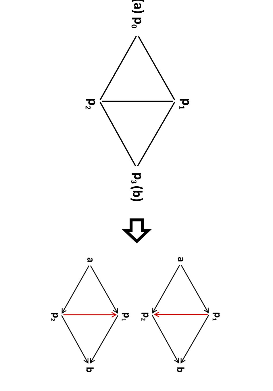
To better formalize the routing strategy, let us exploit the notions of in- and out-neighborhoods. Given an orientation of , we have a corresponding flow network, denoted by , where is the set of directed edges. For arbitrary point , we define its out-neighborhood as the set of heads going from
| (93) |
and its in-neighborhood as the set of tails going into
| (94) |
A logical multicast from point can be defined as a point-to-multipoint connection from to all its out-neighborhood , i.e., . A multipath routing strategy can therefore be defined as an ordered sequence of all such multicasts. See Fig. 13.
Using these definitions we may easily formalize the multipath network protocol that we may simply call “flooding protocol”. Suppose that we have points in the network ( repeaters plus the two end-points). The first step of the protocol is the agreement of a multipath routing strategy by means of preliminary CCs among all the points. This is part of an initialization LOCC which prepares an initial separable state for the entire network. Then, Alice exchanges quantum systems with all her out-neighborhood . This multicast is followed by a network LOCC . Next, repeater exchanges quantum systems with all its out-neighborhood , which is followed by another LOCC and so on. At some step , Bob will have exchanged quantum systems with all his in-neighborhood , after which there is a final LOCC . This completes the first multipath transmission between the end-points by means of the routing and the sequence of LOCCs . Then, there will be the second use of the network with a generally different routing strategy , and so on. See Fig. 14.

Let us note that the points of the network may generally update their routing strategy “on the fly”, i.e., while the protocol is running; then, the various multicasts may be suitably permuted in their order. In any case, for large number of uses , we will have a sequence of multipath routings and network LOCCs whose output provides Alice and Bob’s final state . The flooding protocol will be fully described by and . By definition, its average rate is if , where is a target state of bits. The multipath capacity of the network is defined by optimizing the asymptotic rate over all flooding protocols, i.e.,
| (95) |
By specifying the target state, we define corresponding capacities for quantum communication, entanglement distillation, key generation and private communication, satisfying
| (96) |
Before proceeding, some other considerations are in order. Note that the parallel uses of the network may also be re-arranged in such a way that each point performs all its multicasts before another point. For instance, in the example of Fig. 14, we may consider Alice performing all her multicasts as a first step. Suppose that routes and are chosen with probability and . Then, after Alice has finished, point performs its multicasts and performs its multicasts, and so on. We may always re-arrange the protocol and adapt the LOCC sequence to include this variant.
Then, there is a simplified formulation to keep in mind. In fact, a special case is when the various multicasts within the same routing strategy are not alternated with network LOCCs but they are all performed simultaneously, with only the initial and final LOCCs to be applied. For instance, for the routing of Fig. 14, this means to set and assume that the multicasts , and occur simultaneously, after the initialization and before . In general, any variant of the protocol may be considered as long as each quantum channel (edge) is used exactly times at the end of the communication, i.e., after uses of the quantum network.
In the following section, we show how to simulate a quantum network and then exploit teleportation stretching to reduce adaptive protocols (based on single- or multi-path routings) into much simpler block versions. By combining this technique with entanglement cuts of the quantum network, we will derive very useful decompositions for Alice and Bob’s output state. These decompositions will be later exploited in Secs. VII and VIII to derive single-letter upper bounds for the network capacities and . Corresponding lower bounds will also be derived by combining point-to-point quantum protocols with classical routing strategies, with exact results for distillable networks.
VI Simulation and stretching of a quantum network
VI.1 General approach
Consider a quantum network which is connected by arbitrary quantum channels. Given two points and connected by channel , we consider its simulation for some LOCC and resource state . Repeating this for all connected points , we define an LOCC simulation of the entire network and a corresponding resource representation of the network . For a network of teleportation-covariant channels, its simulation is based on teleportation over Choi matrices, so that we may consider , i.e., we have a “Choi-representation” of the network. Note that the simulation may be asymptotic for a network of bosonic channels, following the same treatment previously explained for a linear chain of repeaters .
By adopting a network simulation , we may apply simplify adaptive protocols via teleportation stretching, by extending the procedure employed for a linear chain of quantum repeaters, with the important difference that we now have many possible chains (the network routes) and these may also have collisions, i.e., repeaters and channels in common. The stretching of a quantum network is performed iteratively, i.e., transmission after transmission. Suppose that the th transmission in the network occurs between points and via channel with associated resource state . Call the global state of the network after this transmission. Then, we may write
| (97) |
where is a trace-preserving LOCC (see also Fig. 15).

By iterating Eq. (97) and considering that the initial state of network is separable, we may then write the network output state after transmissions as
| (98) |
where is the number of uses of channel or, equivalently, edge . Then, by tracing out all the points but Alice and Bob, we get their final shared state
| (99) |
for another trace-preserving LOCC .
Note that the decompositions of Eqs. (98) and (99) can be written for any adaptive network protocol (sequential or flooding). For a sequential protocol , where is the probability of using edge . For a flooding protocol, we instead have , because each edge is used exactly once in each end-to-end transmission. In particular, in a flooding protocol, we have the parallel use of several channels , , … in each multicast, which means that trivial LOCCs (identities) are applied between every two transmissions in the same multicast. We have therefore proven the following result (see also Fig. 16 for a simple example).
Lemma 8 (Network stretching)
Consider a quantum network which is simulable with some resource representation . Then, consider uses of an adaptive protocol so that edge is used times. We may write the global output state of the network as
| (100) |
for a trace-preserving LOCC . Similarly, Alice and Bob’s output state is given by Eq. (100) up to a different trace-preserving LOCC . In particular, we have () for a sequential (flooding) protocol. Formulations may be asymptotic for bosonic channels.

As we state in the lemma, the stretching procedure also applies to networks of bosonic channels with asymptotic simulations. This can be understood by extending the argument already given for linear chains. For the sake of clarity, we make this argument explicit here. Consider again the th transmission in the network occurring via channel as in Fig. 15. For the global state of the network, we may write
| (101) |
Suppose that we replace each channel in the network with an approximation , with point-wise limit , meaning that for any state . We may build the approximate network state
| (102) |
Now assume that all the registers in the network are bounded by a large but finite mean number of photons , so that we may write in the energy-bounded diamond norm defined in Eq. (37). By using the monotonicity under CPTP maps and the triangular inequality, we then compute
| (103) |
By iterating the previous formula for all the transmissions in the network, we derive
| (104) |
This distance goes to zero in for any number of uses , any finite number of edges , and any energy .
Now suppose that the approximate channel has an LOCC simulation with some resource state . Then, we may write the approximate network stretching
| (105) |
for a trace-preserving LOCC . Combining Eqs. (104) and (105), we may therefore write the asymptotic version of network stretching
| (106) |
where the limit in is intended in trace norm and holds for any finite , and .
VI.2 Network stretching with entanglement cuts
We may achieve a non-trivial simplification of previous Lemma 8 in such a way that we greatly reduce the number of resource states in the decomposition of Alice and Bob’s output state . This is possible using Alice-Bob entanglement cuts of the quantum network. These types of cuts will enable us to include many resource states in Alice’s and Bob’s LOs, while preserving the locality between the two end-points.
By definition, an Alice-Bob entanglement cut of the quantum network is a bipartition of all the points of the network such that and . Then, the cut-set of is the set of edges with one end-point in each subset of the bipartition, so that the removal of these edges disconnects the network. Explicitly,
| (107) |
Note that the cut-set identifies an ensemble of channels . Similarly, we may define the following complementary sets
| (108) | ||||
| (109) |
so that .
To simplify the stretching of the network, we then adopt the following procedure. Given an arbitrary cut , we extend Alice and Bob to their corresponding partitions. This means that we consider super-Alice with global register , and super-Bob with global register . Then, all the resource states are included in the LOs of super-Alice, and all those are included in the LOs of super-Bob. Note that the only resource states not absorbed in LOs are those in the cut-set . These states are the only ones responsible for distributing entanglement between the super-parties. The inclusion of all the other resource states into the global LOCC leads to another trace-preserving quantum operation which remains local with respect to and . Thus, for any cut , we may write the following output state for super-Alice and Bob after uses of an adaptive protocol
| (110) |
The next step is tracing out all registers but the original Alice’s and Bob’s . This operation preserves the locality between and . In other words, we may write the following reduced output state for the two end-points
| (111) |
where is a trace-preserving LOCC. All these reasonings automatically transform Lemma 8 into the following improved Lemma. See also Fig. 17 for an example.
Lemma 9 (Network stretching with cuts)
Consider a quantum network simulable with a resource representation . For a teleportation-covariant network, is a Choi-representation, i.e., . Then, consider uses of an adaptive protocol so that edge is used times. For any entanglement cut and corresponding cut-set , we may write Alice and Bob’s output state as
| (112) |
for a trace-preserving LOCC . In particular, we have () for a sequential (flooding) protocol. Formulations may be asymptotic for bosonic channels.
As stated in this improved lemma, the decomposition in Eq. (112) can be extended to networks of bosonic channels with asymptotic simulations. We can adapt the previous reasoning to find the cut-version of Eq. (106), i.e., the trace-norm limit
| (113) |
for suitable sequences of trace-preserving LOCC and resource states (with the result holding for any , number of edges and mean number of photons ).
With Lemma 9 in our hands, we have the necessary tool to derive our single-letter upper bounds for the single- and multi-path capacities of an arbitrary quantum network. This tool needs to be combined with a general weak converse upper bound based on the REE. In the following section, we derive our results for the case of single-path routing over the network. The results for multipath routing will be given in Sec. VIII. In these sections, the upper bounds will be combined with suitable lower bounds that are derived by mixing point-to-point quantum protocols with classical routing strategies (widest path and maximum flow of a network).

VII Results for single-path routing
VII.1 Converse part (upper bound)
In order to write a single-letter upper bound for the single-path capacity of the quantum network, we need to introduce the notion of REE flowing through a cut under some simulation. Consider an arbitrary quantum network with a resource representation . Then, consider an arbitrary entanglement cut with corresponding cut-set . Under the simulation considered, we define the single-edge flow of REE through the cut as the following quantity
| (114) |
By minimizing over all possible entanglement cuts of the network, we build our upper bound for the single-path capacity. In fact, we may prove the following.
Theorem 10 (Converse for single-path capacity)
Consider an arbitrary quantum network with some resource representation . In particular, may be a Choi-representation for a teleportation-covariant network. Then, the single-path capacity of must satisfy the single-letter bound
| (115) |
where the single-edge flow of REE in Eq. (114) is minimized across all cuts of the network. Formulations may be asymptotic for networks of bosonic channels.
Proof. According to Eq. (91) the single-path capacity is defined by the following optimization of the asymptotic rate over the sequential protocols
| (116) |
We can directly extend the general weak-converse in Theorem 1 from channels to networks. This means to replace the supremum over point-to-point protocols with a supremum over network sequential protocols , i.e.,
| (117) |
The other elements of this bound are unchanged because they are exclusively based on the fact that the output state is (by definition) epsilon close to a target state.
According to previous Lemma 9, for any sequential protocol and entanglement cut of the network, we may write Eq. (112). Computing the REE on this decomposition and exploiting basic properties (monotonicity of REE under and subadditivity over tensor products), we derive the following inequality
| (118) |
where and being the probability of using edge according to protocol . By maximizing over the convex combination, we get rid of and write
| (119) |
By using Eq. (119) in Eq. (117), we see that both the optimization over and the limit over disappear, and we are left with the bound
| (120) |
By minimizing over all cuts, we therefore prove Eq. (115).
Note that, from Eq. (118) we may also derive
| (121) |
where is the optimal use of edge over all possible . Here represents the average flow of REE through under the chosen simulation and optimized over . By minimizing over all cuts, we get
| (122) |
This may be tighter than Eq. (115) but difficult to compute due to residual optimization over the protocols.
Finally, note that Eq. (115) can be extended to considering asymptotic simulations, following the same ideas in the proof of Theorem 7. Let us compute the REE on the asymptotic state of Eq. (113). We may write
| (123) |
where: (1) is a generic sequence of separable states converging in trace norm, i.e., such that there is a separable state so that ; (2) we use the lower semi-continuity of the relative entropy [52]; (3) we use that are specific types of converging separable sequences within the set of all such sequences; (4) we use the monotonicity of the relative entropy under trace-preserving LOCCs; (5) we use the definition of REE for asymptotic states ; (6) we use the subadditivity over tensor products.
VII.2 Direct part (achievable rate)
In this section, we derive an achievable asymptotic rate for the end-to-end quantum/private communication via single-path routing. This rate will provide a lower bound to the single-path capacity of an arbitrary quantum network, i.e., with arbitrary topology and arbitrary quantum channels. The non-trivial result is that the achievable rate can be written in terms of a capacity minimized over the entanglement cuts in the network. This step will allow us to exactly establish the single-path capacity of distillable networks in the next subsection.
Consider an arbitrary quantum network where edge is connected by channel with associated two-way capacity . Given an arbitrary entanglement cut of the network, we define its single-edge capacity as the maximum number of target bits distributed by a single edge across the cut, i.e.,
| (124) |
A minimum cut is such that
| (125) |
Then, given a route with an associated chain of channels , we define its capacity as the minimum capacity among its channels, i.e.,
| (126) |
An optimal route is such that
| (127) |
It is clear that is an achievable end-to-end rate. In fact, consider independent point-to-point protocols between pairs of consecutive points along route . An optimal adaptive protocol between points and (connected by ) achieves the capacity value . Then, by composing all outputs via a network LOCCs (e.g., swapping the distilled states or relaying the secret keys via one-time pad sessions), Alice and Bob obtain an achievable rate of .
Thus, we may write the lower bound . The crucial observation is that this bound is also equal to the minimization in Eq. (125) over all entanglement cuts. In fact, we may prove the following.
Theorem 11 (Lower bound)
Consider an arbitrary quantum network where two end-points are connected by an ensemble of routes and may be disconnected by an entanglement cut . The single-path capacity of the network satisfies
| (128) |
Thus, the capacity of an optimal route not only is an achievable rate but it is also equal to the single-edge capacity of a minimum cut . Furthermore, the optimal route is a simple path within a maximum spanning tree of the network.
Proof. It is easy to show the inequality . In fact, an edge of the optimal route must belong to the cut-set . Thus, the capacity of that edge must simultaneously satisfy and . In order to show the opposite inequality , we need to exploit some basic results from graph theory. Consider the maximum spanning tree of the connected undirected graph . This is a subgraph which connects all the points in such a way that the sum of the capacities associated with each edge is the maximum. In other words, it maximizes the following quantity
| (129) |
Note that the optimal route between Alice and Bob is the unique path between Alice and Bob within this tree [99]. Let us call the critical edge in , i.e., that specific edge which realizes the minimization
| (130) |
Since this edge is part of a spanning tree, there is always an Alice-Bob cut of the network which crosses and no other edges of the spanning tree. In fact, this condition would fail only if there was a cycle in the tree, which is not possible by definition.

Then, we must also have that is the optimal edge in the cut-set , i.e., . By absurd, assume this is not the case. This implies that there is another edge , not belonging to , such that . For the cut property of the maximum spanning trees [96], we have that an edge in with maximum capacity must belong to all the maximum spanning trees of the network. Therefore must belong to which leads to a contradiction. In conclusion, we have found an Alice-Bob cut which realizes the condition . For an example see Fig. 18.
Note that the previous result applies not only to quantum networks but to any graphical weighted network. It is sufficient to replace the capacity of the edge with a generic weight. In fact, Theorem 11 can be restated as follows, which represents a “single-flow” formulation of the max-flow min-cut theorem [65, 66, 67, 59].
Proposition 12 (Cut property of the widest path)
Consider a network described by an undirected graph , whose edge has weight . Denote by the ensemble of undirected paths between the end-points, Alice and Bob. Define the weight of a path as , and the weight of an Alice-Bob cut as . The weight of the widest path is equal to that of the minimum cut
| (131) |
Finding the optimal route in a quantum network (Theorem 11) is equivalent to finding the widest path in a weighted network (Proposition 12), i.e., solving the well-known widest path problem. Using a modified Dijkstra’s shortest path algorithm [64], the solution is found in time . In practical cases, this algorithm can be optimized and its asymptotic performance becomes [97]. Another possibility is using an algorithm for finding a maximum spanning tree of the network, such as the Kruskal’s algorithm [98, 64]. The latter has the asymptotic complexity for building the tree. This step is then followed by the search of the route within the tree which takes linear time [99].
VII.3 Formulas for teleportation-covariant and distillable networks
The results of Theorems 10 and 11 can be specified for quantum networks which are connected by teleportation-covariant channels. Given a teleportation-covariant network whose teleportation simulation has an associated Choi-representation , we may write the following for the single-path capacity
| (132) |
with being defined in Eq. (124), and
| (133) |
The latter may have an asymptotic formulation for networks of bosonic channels, with the REE taking the form as in Eq. (26) over , where is a sequence of Choi approximating states with finite energy.
In particular, consider a network connected by distillable channels. This means that for any edge , we may write (exactly or asymptotically)
| (134) |
By imposing this condition in Eq. (132), we find that upper and lower bounds coincide. We have therefore the following result which establishes the single-path capacity of a distillable network and fully extends the widest path problem [63] to quantum communications.
Corollary 13 (Single-path capacities)
Consider a distillable network , where two end-points are connected by an ensemble of routes and may be disconnected by an entanglement cut . An arbitrary edge is connected by a distillable channel with two-way capacity and Choi matrix . Then, the single-path capacity of the network is equal to
| (135) |
with an implicit asymptotic formulation for bosonic channels. Equivalently, is also equal to the minimum (single-edge) capacity of the entanglement cuts and the maximum capacity of the routes, i.e.,
| (136) |
The optimal end-to-end route achieving the capacity can be found in time , where is the number of edges and is the number of points. Over this route, a capacity-achieving protocol is based on one-way entanglement distillation sessions between consecutive points, followed by entanglement swapping.
The proof of this corollary is a direct application of the previous reasonings. We see that it first reduces the routing problem to a classical optimization problem, i.e., finding the widest path. Then, over this optimal route, the single-path capacity is achieved by a non-adaptive protocol based on one-way CCs. In fact, we have that any two consecutive points and along may distill ebits at the rate of , where is the connecting channel. Then, sessions of entanglement swapping (also based on one-way CCs), distribute ebits at the end-points with a rate of at least . Due to Eq. (134), this rate is equal to , which corresponds to the capacity .
VII.4 Single-path capacities of fundamental networks
Let us specify the result of Corollary 13 to fundamental scenarios such as bosonic networks subject to pure-loss or quantum-limited amplification, or spin networks affected by dephasing or erasure. These are in fact all distillable networks. We find extremely simple formulas for their single-path capacities, setting their ultimate limit for quantum communication, entanglement distribution, key generation and private communication under single-path routing.
Start with a network connected by lossy channels , which well describes both free-space or fiber-based optical communications. According to Corollary 13, we may compute its capacity by minimizing over the cuts or maximizing over the routes. Generic edge has an associated lossy channel with transmissivity and capacity . Therefore, an entanglement cut has single-edge capacity
| (137) |
where may be identified as the (single-edge) transmissivity of the cut. By minimizing over the cuts, we may write the single-path capacity of the lossy network as
| (138) |
where is the minimum transmissivity of the cuts.
Consider now a generic end-to-end route along the lossy network. This route is associated with a sequence of lossy channels with transmissivities . We then compute the route capacity as
| (139) |
where is the route transmissivity. By maximizing over the routes, we may equivalently write the single-path capacity of the lossy network as
| (140) |
where is the maximum transmissivity of the routes.
Similar conclusions can be derived for bosonic networks which are composed of other distillable Gaussian channels, such as multiband lossy channels, quantum-limited amplifiers or even hybrid combinations. In particular, consider a network of quantum-limited amplifiers , where the generic edge has gain with capacity , and the generic end-to-end route is associated with a sequence of gains . We can repeat the previous steps of the lossy network but setting , so that . Thus, for an entanglement cut , we may write
| (141) |
For a route , we have the capacity
| (142) |
By minimizing over the cuts or maximizing over the routes, we derive the two equivalent formulas
| (143) |
where and .
We can also compute the single-path capacities of DV networks where links between qudits are affected by dephasing or erasure or a mix of the two errors. For simplicity, consider the case of qubits, such as spin or polarized photons. In a qubit network with dephasing channels , the generic edge has a dephasing probability and capacity . The generic end-to-end route is associated with a sequence of such dephasing probabilities . For an entanglement cut , we have
| (144) |
For a generic route , we may write
| (145) |
By minimizing over the cuts or maximizing over the routes, we then derive the single-path capacity
| (146) |
where we have set
| (147) |
Finally, for a qubit network affected by erasures we have that edge is associated with an erasure channel with probability and corresponding capacity . As a result, we may repeat all the previous derivation for the dephasing network up to replacing with . For a cut and a route, we have
| (148) |
where and are defined as in Eqs. (144) and (145). Thus, the single-path capacity of the erasure network simply reads
| (149) |
where and are defined as in Eq. (147).
VIII Results for multipath routing
VIII.1 Converse part (upper bound)
In order to write a single-letter upper bound for the multipath capacity of a quantum network, we need to introduce the concept of multi-edge flow of REE through a cut, under some simulation of the network. Consider an arbitrary quantum network whose simulation has an associate resource representation . Then, consider an arbitrary entanglement cut with corresponding cut-set . Under the simulation considered, we define the multi-edge flow of REE through the cut as the following quantity
| (150) |
By minimizing over all possible entanglement cuts of the network, we build our upper bound for the multipath capacity. In fact, we may prove the following.
Theorem 14 (Converse for multi-path capacity)
Consider an arbitrary quantum network with some resource representation . In particular, may be a Choi-representation for a teleportation-covariant network. Then, the multipath capacity of must satisfy the single-letter bound
| (151) |
where the multi-edge flow of REE in Eq. (150) is minimized across all cuts of the network. Formulations may be asymptotic for networks of bosonic channels.
Proof. According to Eq. (95) the multipath capacity is defined by the following optimization of the asymptotic rate over the flooding protocols
| (152) |
Let us apply the weak-converse in Theorem 1 by replacing the supremum over point-to-point protocols with a supremum over flooding protocols , i.e.,
| (153) |
According to previous Lemma 9, for any flooding protocol and entanglement cut , we may write Eq. (112) with . Computing the REE on this decomposition and exploiting basic properties of the REE, we derive
| (154) |
By using Eq. (154) in Eq. (153), both the supremum and the limit disappear, and we are left with the bound
| (155) |
By minimizing over all cuts, we therefore prove Eq. (151). The extension to asymptotic simulations follows the same derivation in the proof of Theorem 10 but setting . We find again Eq. (151) but where the REE takes the weaker formulation for asymptotic states of Eq. (26).
VIII.2 Direct part (achievable rate)
We now provide a general lower bound to the multipath capacity. Consider an arbitrary quantum network where edge is connected by channel with two-way capacity . Given an arbitrary entanglement cut of the network, we define its multi-edge capacity as the total number of target bits distributed by all the edges across the cut, i.e.,
| (156) |
In this setting, a minimum cut is such that
| (157) |
We now prove that the later is an achievable rate for multipath quantum/private communication.
Theorem 15 (Lower bound)
Consider an arbitrary quantum network where two end-points may be disconnected by an entanglement cut . The multipath capacity of the network satisfies
| (158) |
In other words, the minimum multi-edge capacity of the entanglement cuts is an achievable rate. This rate is achieved by a flooding protocol whose multipath routing can be found in time by solving the classical maximum flow problem.
Proof. To show the achievability of the rate in Eq. (157), we resort to the classical max-flow min-cut theorem [66]. In the literature, this theorem has been widely adopted for the study of directed graphs. In general, it can also be applied to directed multi-graphs as well as undirected graphs/multi-graphs (e.g., see [59, Sec. 6]). The latter cases can be treated by splitting the undirected edges into directed ones (e.g., see [59, Sec. 2.4]).
Our first step is therefore the transformation of the undirected graph of the quantum network into a suitable directed graph (in general, these may be multi-graphs, in which case the following derivation still holds but with more technical notation). Starting from , we consider the directed graph where Alice’s edges are all out-going (so that she is a source), while Bob’s edges are all in-going (so that he is a sink). Then, for any pair and of intermediate points , we split the undirected edge into two directed edges and , having capacities equal to the capacity of the original undirected edge [100]. These manipulations generate our flow network . See Fig. 19 for an example.

We then adopt the standard definition of cut-set for flow networks, here called “directed cut-set”. Given an Alice-Bob cut of the flow network, with bipartition of the points , its directed cut-set is defined as . This means that directed edges of the type do not belong to this set (see Fig. 19). Using this definition, the cut-properties of the flow network are exactly the same as those of the original undirected graph , for which we used the “undirected” definition of cut-set. For this reason, we have
| (159) |
where the first quantity is computed on , while the second one is computed on the flow network . We aim to show that the latter is an achievable rate.
Let us now define the “flow” in the network as the number of qubits per use which are reliably transmitted from to along the directed edge , denoted by . This quantum transmission is performed by means of a point-to-point protocol where and exploit adaptive LOCCs, i.e., unlimited two-way CCs and adaptive LOs, without the help of the other points of the network. It is therefore bounded by the two-way quantum capacity of the associated channel , i.e., . The actual physical direction of the quantum channel does not matter since it is used with two-way CCs, so that the two points and first distill entanglement and then they teleport qubits in the “logical direction” specified by the directed edge.
Since every directed edge between two intermediate points has an opposite counterpart , we may simultaneously consider an opposite flow of qubits from to with rate . As a result, there will be an “effective” point-to-point rate between and which is defined by the difference of the two “directed” rates
| (160) |
Its absolute value provides the effective number of qubits transmitted between to per use of the undirected edge. For , effective qubits flow from to , while means that effective qubits flow from to . The effective rate is correctly bounded and we set if two points are not connected. The ensemble of positive directed rates represents a flow vector in . For any choice of this vector, there is a corresponding ensemble of effective rates for the original network . The signs specify an orientation for , and the absolute values provide point-to-point quantum communication rates for the associated protocol.
It is important to note that represents a “legal” flow vector in only if we impose the property of flow conservation [59]. This property can be stated for or, equivalently, for the effective vector . At any intermediate point, the number of qubits simultaneously received must be equal to the number of qubits simultaneously transmitted through all the point-to-point communications with neighbor points. In other words, for any , we must impose
| (161) |
This property does not hold for Alice (source) and Bob (sink), for which we impose
where is known as the value of the flow. This is an achievable end-to-end rate since it represents the total number of qubits per network use which are transmitted by Alice and correspondingly received by Bob via all the end-to-end routes, where the intermediate points quantum-communicate at the rates .
Now, from the classical max-flow min-cut theorem, we know that the maximum value of the flow in the network is equal to the capacity of the minimum cut [66, 59], i.e., we may write
| (162) |
Thus, by construction, we have that is an achievable rate for quantum communication. The previous reasoning can be repeated for private bits by defining a corresponding flow of private information through the network. Thus, in general, we may write that
| (163) |
is an achievable rate for any of the quantum tasks. This proves that Eq. (159) is an achievable rate.
In order to better understand the flooding protocol that achieves , call the optimal flow vector in . There is a corresponding vector which determines an optimal orientation for the quantum network , besides providing the optimal rates to be reached by the point-to-point connections. In other words, starting from the capacities , the points solve the maximum flow problem and establish an optimal multipath routing . After this, each point multicasts to its out-neighborhood , according to the optimal rates and the optimal orientation.
In conclusion, let us discuss the complexity of finding the optimal multipath routing . By construction, the flow network has only a small overhead with respect to the original network . In fact, we just have . Within , the maximum flow can be found with classical algorithms. If the capacities are rational, we can apply the Ford-Fulkerson algorithm [66] or the Edmonds–Karp algorithm [68], the latter running in time. An alternative is Dinic’s algorithm [69], which runs in time. More powerful algorithms are available [70, 71, 72] and the best running performance is currently time [73, 74]. Thus, adopting Orlin’s algorithm [74], we find the solution in time.
VIII.3 Formulas for teleportation-covariant and distillable networks
Consider a teleportation-covariant quantum network whose teleportation simulation has an associated Choi-representation . Then, from Theorems 14 and 15, we may write the following sandwich for the multipath capacity
| (164) |
with being defined in Eq. (156), and
| (165) |
As usual, the latter may have an asymptotic formulation for networks of bosonic channels, with the REE taking the form as in Eq. (26) over , where is a sequence of states with finite energy.
In particular, consider now a distillable network. This means that, for any edge , we may write Eq. (134), exactly or asymptotically. By imposing this condition in Eq. (164), we find that upper and lower bounds coincide. We have therefore the following result which establishes the multipath capacity of a distillable network and fully extends the max-flow min-cut theorem [65, 66, 67] to quantum communications.
Corollary 16 (Multi-path capacities)
Consider a distillable network , whose arbitrary edge is connected by a distillable channel with two-way capacity and Choi matrix . Then, the multipath capacity of the network is equal to
| (166) |
with an implicit asymptotic formulation for bosonic channels. Equivalently, is also equal to the minimum (multi-edge) capacity of the entanglement cuts
| (167) |
The optimal multipath routing can be found in time by solving the classical maximum flow problem. A capacity-achieving flooding protocol corresponds to performing one-way entanglement distillation between neighbor points, followed by multiple sessions of teleportation in the direction of the optimal network orientation.
The proof is a direct application of the previous reasonings. In particular, from Theorem 15, we have that the routing problem is reduced to the solution of a classical optimization problem, i.e., finding the maximum flow in a flow network. This solution provides an optimal orientation of the quantum network and also the point-to-point rates to be used in the various multicasts. Under this optimal routing, the multipath capacity is achieved by a non-adaptive flooding protocol based on one-way CCs. In fact, because the channels are distillable, each pair of points and may distill ebits. By using the distilled ebits, Alice’s qubits are teleported to Bob along the multipath routes associated with the maximum flow. Since Alice’s qubits can be part of ebits and, therefore, private bits, this protocol can also distill entanglement and keys at the same end-to-end rate.
Thus, Corollary 16 reduces the computation of the multipath capacity of a distillable quantum network to the determination of the maximum flow in a classical network. In this sense the max-flow min-cut theorem is extended from classical to quantum communications. In particular, the distillable network can always be transformed in a teleportation network, where quantum information is teleported as a flow from Alice to Bob.
VIII.4 Multipath capacities of fundamental networks
Consider the practical scenario of quantum optical communications affected by loss, e.g., free-space or fiber-based. A specific distillable network is a bosonic network connected by lossy channels , so that each undirected edge has an associated lossy channel with transmissivity or equivalent “loss parameter” . We may then apply Corollary 16 and express the multipath capacity in terms of the loss parameters of the network.
Let us define the loss of an Alice-Bob entanglement cut as the product of the loss parameters of the channels in the cut-set, i.e., we set
| (168) |
This quantity determines the multi-edge capacity of the cut, since we have . By applying Eq. (167), we find that the multipath capacity of the lossy network is given by
| (169) |
Thus, we may define the total loss of the network as the maximization of over all cuts, i.e.,
| (170) |
and write the simple formula
| (171) |
In general, we may consider a multiband lossy network , where each edge represents a multiband lossy channel with bandwidth and constant transmissivity . In other words, each single edge corresponds to independent lossy channels with the same transmissivity . In this case, we have and we write
| (172) |
which directly generalizes Eq. (171).
In particular, suppose that we have the same loss in each edge of the multiband network, i.e., for any , which may occur when points and are equidistant. Then, we may simply write
| (173) | ||||
| (174) |
where is the effective bandwidth of the network.
Consider now other types of distillable networks. Start with a bosonic network of quantum-limited amplifiers , where the generic edge has an associated gain . Its multipath capacity is given by
| (175) |
For a qubit network of dephasing channels , where the generic edge has dephasing probability , we may write the multipath capacity
| (176) |
Finally, for a qubit network of erasure channels with erasure probabilities , we simply have
| (177) |
Similar expressions may be derived for qudit networks of dephasing and erasure channels in arbitrary dimension.
IX Generalization to multiple senders and receivers
Previous results have been derived in the unicast setting, with a single sender and a single receiver . In general, we may consider the presence of multiple senders and receivers , which may simultaneously communicate according to various configurations. For simplicity, these sets are intended to be disjoint , so that an end-point cannot be sender and receiver at the same time. It is clear that all previous results derived for the two basic routing strategies provide general upper bounds which are still valid for the individual end-to-end capacities associated with each sender-receiver pair in the various settings with multiple end-points.
In the following sections, we start with the multiple-unicast quantum network. This consists of Alices and Bobs , with the generic th Alice communicating with a corresponding th Bob . This case can be studied by assuming single-path routing (IX.1) or multipath routing (IX.2). Besides the general bounds inherited from the unicast scenario, we also derive a specific set of upper bounds for the rates that are simultaneously achievable by all parties.
Another important case is the multicast quantum network, where a single sender simultaneously communicates with receivers, e.g., for distributing different keys. By its nature, this is studied under multipath routing (Sec. IX.3). In this setting, an interesting variant is the distribution of the same key to all receivers, which may be assisted by network coding [57] (Sec. IX.4).
More generally, we may consider a multiple-multicast quantum network. Here we have senders and receivers, and each sender communicates simultaneously with the entire set of receivers (Sec. IX.5). In a private communication scenario, this corresponds to the distribution of different keys. For a description of these configurations, see the simple example of the butterfly quantum network in Fig. 20.

IX.1 Multiple-unicast quantum networks with single-path routing
The generalization to a multiple-unicast setting is relatively easy. Let us start by considering two Alice-Bob pairs and , since the extension to arbitrary number of pairs is immediate. We may easily formulate network protocols which are based on single-path routing. In this case, each sequential use of the network involves the transmission of quantum systems along two (potentially-overlapping) routes
| (178) |
where each transmission through an edge is assisted by network LOCCs. The routes are updated use after use.
After uses, the output of the double-unicast network protocol is a state which is -close in trace norm to a target state
| (179) |
where is a one-bit state (private bit or ebit) for the pair and the number of its copies. Taking the limit of large and optimizing over all protocols , we define the capacity region as the closure of the set of the achievable asymptotic rates . In general, for sender-receiver pairs, we have an -tuple of achievable rates . Depending on the task of the protocol (i.e., the target state), these rates refer to end-to-end entanglement distillation (equivalently, error-free quantum communication) or secret-key generation.
Before proceeding, let us first introduce more general types of entanglement cuts of the quantum network. Given two sets of senders and receivers , we adopt the notation for a cut such that and . Similarly, we write for a cut with and , and for a cut with and . As usual, we consider the single-edge flow of REE trough a cut as
| (180) |
where is a resource state associated with an edge in the cut-set , under some simulation of the network. We can now state the following result.
Theorem 17 (Multi-unicast with single paths)
Let us consider a multiple-unicast quantum network with sender-receiver pairs communicating by means of single-path routing. Adopt a simulation of the network with a resource representation . In particular, can be a Choi-representation for a teleportation-covariant . We have the following outer bounds for the capacity region
| (181) | ||||
| (182) | ||||
| (183) | ||||
where is the single-edge flow of REE through cut . It is understood that formulations may be asymptotic for quantum networks with bosonic channels.
Proof. For simplicity consider first the case , since the generalization to arbitrary is straightforward. Let us also consider key generation, since it automatically provides an upper bound for all the other tasks. Considering the bipartition , the distillable key of the target state in Eq. (179) is equal to
| (184) |
Using the REE with respect to the same bipartition, we may write the upper bound
| (185) |
where the latter inequality comes from the fact that is -close to . The extra term depends the -closeness, and the dimension of the total Hilbert space. In the limit of large and small (weak converse), we can neglect . This is a straightforward application of the exponential scaling of the dimension shown in Refs. [80, 81] for DV systems and extended to CV systems via standard truncation arguments, e.g., see Ref. [26, arXiv version 2 (Dec 2015)] for a simple proof and the discussion in Ref. [78]. As a result we may write
| (186) |
By simulating and stretching the network, we may write the following decomposition of the output state
| (187) |
where is the number of uses of edge and is a trace-preserving LOCC, which is local with respect to the bipartition . By inserting entanglement cuts which disconnect the senders and receivers, we reduce the number of resource states appearing in Eq. (187) while preserving the locality of the LOCC with respect to the bipartition of the end-points. In other words, for any cut we may write
| (188) |
Using the latter decomposition in Eq. (186), we obtain
| (189) |
By minimizing over the cuts, we derive
| (190) |
It is important to note that this bound holds for any protocol , whose details are all collapsed in the LOCC and therefore discarded. Thus, the same bound applies if we optimize over all protocols, which means that Eq. (190) provides the following outer bound for the capacity region
| (191) |
Note that, besides this bound, we also have the following unicast bounds for the individual rates
| (192) |
These follows directly from Theorem 10 on the converse for unicast quantum networks. Equivalently, we may re-derive these bounds here, by setting or in the target state of Eq. (179) and repeating the previous derivation. For instance, for , we have , where does not contain target bits and may be taken to be separable. Therefore, we start from and we repeat all the derivation with respect to the bipartition .
It is clear that the generalization from to arbitrary is immediate. For any integer , we have the target state
| (193) |
Considering the bipartition and the corresponding cuts of the network leads to
| (194) |
where we note that increasing the number of rates reduces the number of possible cuts in the minimization. In order to get all the remaining inequalities of the theorem, we just need to set some of the rates to zero. For instance, for and , we get the unicast bounds of Eq. (181). For , and we get the double-unicast bounds of Eq. (182), and so on. The extension to asymptotic simulations of bosonic channels is achieved by adopting the weaker definition of the REE as in Eq. (26).
Once we have proven the previous theorem, it is immediate to specify the results for the case of multiple-unicast distillable networks, for which we may write for each edge , where is the two-way capacity of the associated quantum channel . In this case, we may directly write
| (195) |
where is the single-edge capacity of cut , already introduced in Eq. (124) for the unicast quantum network. Thus, we may express the bounds of Theorem 17 directly in terms of the capacities of the cuts, i.e., we automatically prove the following.
Corollary 18
Consider a multiple-unicast quantum network with sender-receiver pairs communicating by means of single-path routing. If the network is distillable, then we may write the following outer bounds for the capacity region
| (196) | ||||
| (197) | ||||
| (198) | ||||
where is the single-edge capacity of cut .
Note that we cannot establish the achievability of the outer bounds in Eqs. (196)-(198), apart from the case . This case in fact corresponds to a unicast distillable network for which the bound is achievable by solving the widest path problem (see Corollary 13). In general, for , achievable lower bounds can be established by combining the point-to-point composition strategies with classical routing algorithms that solve the multiple-version of the widest path problem.
IX.2 Multiple-unicast quantum networks with mutipath routing
Here we consider a quantum network where senders and receivers communicate in a pairwise fashion by means of multipath routing. As usual in a multipath protocol, the points first agree an orientation for the quantum network. For multiple-unicasts note that both the senders and receivers may assists one with each other as relays of the network. This means that are not necessarily sources and are not necessarily sinks, i.e., these sets may have both incoming and outgoing edges. Given an orientation, each point multicasts to its out-neighborhood with the assistance of network LOCCs. This flooding process ends when each edge of the network has been exploited. For the next use, the points may agree a different orientation, and so on.
The sequence of the orientations together with the sequence of all network LOCCs (exploited in each orientation) define a multiple-unicast flooding protocol . Its output will be a shared state which is -close to a target state
| (199) |
where is a one-bit state (private bit or ebit) for the pair and the number of its copies. By taking the limit of large and optimizing over , we define the capacity region associated with the achievable rates for the various quantum tasks. We can state the following result.
Theorem 19 (Multi-unicast with multipaths)
Let us consider a multiple-unicast quantum network with sender-receiver pairs communicating via multipath routing. Adopt a simulation of the network with a resource representation . In particular, can be a Choi-representation for a teleportation-covariant . We have the following outer bounds for the capacity region
| (200) | ||||
| (201) | ||||
| (202) | ||||
where is the multi-edge flow of REE across cut as in Eq. (150). It is understood that formulations may be asymptotic for quantum networks with bosonic channels.
Proof. The proof follows the main steps of the one of Theorem 17. As before, consider key generation. For the bipartition , the distillable key of the target state is equal to
| (203) | ||||
| (204) | ||||
| (205) |
which leads to the inequality
| (206) |
For any cut of the (simulated) network, we may write the following decomposition of the output state
| (207) |
for some trace-preserving LOCC . Note that here we have . By replacing in Eq. (206), we therefore get
| (208) |
The next step is to minimize over the cuts, leading to
| (209) |
Since the latter inequality holds for any protocol , it can be extended to the achievable rates, i.e., we write
| (210) |
Finally, by setting some of the rates equal to zero in the target state, we may repeat the procedure with respect to different bipartitions and derive all the remaining conditions in Eqs. (200)-(202). The extension to asymptotic simulations of bosonic channels is achieved by adopting the weaker definition of the REE as in Eq. (26).
It is immediate to specify the result for distillable networks for which we may directly write
| (211) |
where is the multi-edge capacity of cut , already introduced in Eq. (156). We may write the following.
Corollary 20
Consider a multiple-unicast quantum network with sender-receiver pairs communicating via multipath routing. If the network is distillable, then we may write the following outer bounds for the capacity region
| (212) | ||||
| (213) | ||||
| (214) | ||||
where is the multi-edge capacity of cut .
Achievable lower bounds may be determined by combining the point-to-point composition strategy with classical routing algorithms based on the maximization of multiple flows. For the specific case , the outer bound is achievable and we retrieve the max-flow min-cut theorem for quantum communications (see Corollary 16). For , achievable lower bounds may be found by exploiting classical literature on multicommodity flow algorithms, e.g., Ref. [101] who showed a version of max-flow min-cut theorem for undirected networks with two commodities, and Ref. [56] which discusses extensions to more than two commodities.
IX.3 Multicast quantum networks
Let us now consider a multicast scenario, where Alice aims at simultaneously communicate with a set of receivers, i.e., a set of Bobs . Because of the implicit parallel nature of this communication process, it is directly formulated under the assumption of multipath routing. We can easily generalize the description of the one-sender one-receiver flooding protocol to the present case of multiple receivers.
In a -to- multicast network protocol, the quantum network is subject to an orientation where Alice is treated as a source, while the various Bobs are destination points, each one being a receiver but also a potential relay for another receiver (so that they are not necessarily sinks in the general case). Each end-to-end simultaneous communication between Alice and the Bobs consists of a sequence of multicasts from each point of the network to its out-neighborhood, assisted by network LOCCs. This is done in a flooding fashion so that each edge of the network is exploited. The orientation of the network may be updated and optimized at each round of the protocol.
The sequence of orientations and the network LOCCs define the multicast flooding protocol . After uses of the network, Alice and the Bobs will share an output state which is -close to a target state
| (215) |
where is a one-bit state (private bit or ebit) for the pair of points and the number of its copies. Note that this is a compact notation which involves countable sets of systems and . Therefore, the tensor product explicitly means , so that there are different systems involved in Alice’s side.
By taking the limit of large and optimizing over , we define the capacity region associated with the achievable rates . In particular, we may define a unique capacity which is associated with the symmetric condition . In fact, we may consider a symmetric type of protocol whose target state must have bits for any . Then, by taking the asymptotic limit of large and maximizing over all such protocols, we may define the multicast network capacity
| (216) |
This rate quantifies the maximum number of target bits per network use (multipath transmission) that Alice may simultaneously share with each Bob in the destination set . We have the usual hierarchy when we specify the target state. We can now state the following general bound.
Theorem 21 (Quantum multicast)
Let us consider a multicast quantum network with one sender and receivers . Adopt a simulation of the network with a resource representation . In particular, can be a Choi-representation for a teleportation-covariant . Then we have the following outer bounds for the capacity region
| (217) | ||||
| (218) | ||||
| (219) | ||||
where is the multi-edge flow of REE through cut . In particular, the multicast network capacity satisfies
| (220) |
It is understood that formulations may be asymptotic for quantum networks with bosonic channels.
Proof. Consider the upper bound given by secret-key generation. With respect to the bipartition , we may write the usual steps starting form the distillable key of the target state
| (221) | ||||
| (222) | ||||
| (223) |
leading to the asymptotic limit
| (224) |
For any cut of the (simulated) network, we may write the decomposition
| (225) |
for some trace-preserving LOCC . By replacing in Eq. (224), we therefore get
| (226) |
By minimizing over the cuts and maximizing over the protocols, we may write
| (227) |
The other conditions in Eqs. (217)-(219) are obtained by setting part of the rates to zero in the target state (as in the previous proofs). In particular, set for some , while for any . The target state becomes and we repeat the derivation with respect to the bipartition . This leads to
| (228) |
where we may directly consider the reduced state
| (229) |
For any cut , we therefore have
| (230) |
which leads to . By minimizing over the cuts, one gets
| (231) |
Since this is true for any protocol , it can be extended to the achievable rates, i.e., we get Eq. (217).
For the multicast network capacity, just note that
| (232) |
Therefore, from Eq. (231), we may write
| (233) |
This is true for any symmetric protocol which leads to the result of Eq. (220). Results are extended to asymptotic simulations of bosonic channels in the usual way.
As usual, in the case of distillable networks, we may prove stronger results. As a direct consequence of Theorem 21, we may write the following cutset bound.
Corollary 22
Consider a multicast quantum network with one sender and receivers . If the network is distillable, then we have the following outer bounds for the capacity region
| (234) | ||||
| (235) | ||||
| (236) | ||||
where is the multi-edge capacity of cut and is the multipath capacity between the sender and the th receiver (in a unicast setting). In particular, the multicast network capacity must satisfy the bound
| (237) |
IX.4 Network coding for quantum key distribution
Our previous results refer to the general case of multiple independent messages. In a multicast quantum network, this means that Alice distributes different sequences of target bits to the Bobs . For instance, these may represent different secret keys, one for each Bob in the destination set. For this specific task (key distribution), the multicast capacity of the network becomes a multicast secret-key capacity .
In quantum key distribution, it is also interesting to consider the variant scenario where Alice distributes exactly the same secret key to all Bobs , for instance, to enable a quantum-secured conference among these parties. For this particular task, we may define a single-key version for the multicast secret-key capacity, that we denote as . This represents the maximum rate at which Alice may distribute the same secret key to all Bobs in each parallel use of the network.
Here some considerations are in order. First of all, it is clear that just because the various Bobs may compose their keys to distil a common key. This also means that the cutset bound in Eq. (237) does not automatically apply to . Another reason for this is because, more generally, we may include the possibility of network coding [57] in the definition of . This means that the intermediate nodes of the network not only help with the multipath routing of the quantum systems from Alice to the Bobs, but they may also apply operations on the incoming systems before their subsequent transmission. For this reason, may be greater than a routing capacity.
In a multicast distillable network, we may therefore combine point-to-point key generation sessions with linear network coding [57]. In this way we may find a lower bound to the single-key multicast capacity by exploiting the network coding theorem [102, 103, 104].
Theorem 23 (Network coding for QKD)
Consider a distillable network . Then, the single-key multicast capacity between one sender and receivers satisfies
| (238) |
where is the multipath secret-key capacity between the sender and the th receiver (in a unicast setting).
Proof. The proof repeats some of the steps of the previous proofs for multipath routing. First of all we transform the quantum network into a directed network where each undirected edge is split in two directed edges. The Alice-Bob cut properties of the original quantum network and the new directed graphical network are exactly the same if we consider a corresponding “directed” definition for the cut-sets. In particular, the cutset bound in Eq. (238) remains the same for the directed network under the re-definition of the cut-sets.
An optimal key distribution protocol goes as follows. The points distill ebits along each (undirected) edge. These ebits are then used to teleport orthogonal states along the directed edges of the oriented graphical network. Let us call Alice’s secret variable, uniformly chosen and encoding bits. After extractions of , we have a sequence of bits. Let us split this sequence into blocks , where each block contains bits. For large , we may always assume that is an integer, so that each block corresponds to an element of the finite field .
The blocks are then subject to a linear coding transformation, i.e., Alice computes the output
| (239) |
with some coefficients . The generic block is encoded into an orthogonal set of pure states and teleported to a neighbor point by means of the shared ebits. Alice communicates both the dimension of the basis and the outcome of the Bell detection to point . The latter will apply the correction unitary and then detect the state with the POVM , so to extract without errors. In this way, the blocks of the sequence are all teleported from Alice to her neighborhood .
In turn, each point of the network will receive a number of teleported states which will be measured and decoded into the blocks of an input sequence . The latter will be subject to linear coding with coefficients and transformed into an output sequence whose blocks are encoded into orthogonal states and then teleported to neighbor points, and so on. In this way, we have transformed the original network into a teleportation network where orthogonal states are used to securely transfer blocks of the secret key through the points of the network, with the only limitation being provided by the point-to-point capacities .
Security is provided by the pre-distillation of the ebits, while the effective secret-key transfer has become equivalent to solving the transfer of classical bits in a directed network, thanks to teleportation. For this reason we can apply the classical network coding theorem [102, 103, 104], which states that the optimal achievable rate is equal to the cutset bound (e.g., see Theorem 15.3 of Ref. [57]). Here, this means that the single-key multicast capacity satisfies the lower bound in Eq. (238).
IX.5 Multiple-multicast quantum networks
In the multiple-multicast quantum network, we have Alices , each of them communicating with the same destination set of Bobs by means of multipath routing. Each end-to-end multicast is associated with the distribution of independent sequences of target bits (e.g., secret keys) between the th Alice and each Bob in the destination set. The description of a multiple-multicast protocol for a quantum network follows the same main features discussed for the case of a single-multicast network (). Because we have multiple senders and receivers, here we need to consider all possible orientations of the network. Each use of the quantum network is performed under some orientation which is adopted by the points for their point-to-point out-neighborhood multicasts, suitably assisted by network LOCCs. Use after use, these steps define a multiple-multicast flooding protocol .
After uses, the ensembles of Alices and Bobs share an output state which is -close to a target state
| (240) |
where is a one-bit state (private bit or ebit) for the pair and the number of its copies. By taking the limit of large and optimizing over , we define the capacity region for the achievable rates . Assume the symmetric case where the th Alice achieves the same rate with all Bobs . This means to consider symmetric protocols whose target state must have bits for any . By taking the asymptotic limit of for large and maximizing over all these symmetric protocols, we may define the capacity region for the achievable multicast rates . In the latter set, rate provides the minimum number of target bits per use that the th Alice may share with each Bob in the destination set (in the multi-message setting, i.e., assuming independent sequences shared with the various Bobs). We have the following outer bounds to the capacity region.
Theorem 24 (Quantum multiple-multicast)
Let us consider a multiple-multicast quantum network where each of the senders communicates with receivers at the multicast rate . Adopt a simulation of with some resource representation , which may be a Choi-representation for a teleportation-covariant . Then, we have the following outer bounds for the capacity region
| (241) | ||||
| (242) | ||||
| (243) | ||||
where is the multi-edge flow of REE through cut . For a distillable network, we may write the bounds in Eqs. (241)-(243) with , i.e., in terms of the multi-edge capacity of the cuts.
Proof. The proof is again similar to previous ones. Consider the upper bound given by secret-key generation. With respect to the bipartition , we can manipulate the distillable key of the target state as follows
| (244) | ||||
| (245) | ||||
| (246) |
leading to the asymptotic limit
| (247) |
For any cut of the (simulated) network, we may write the decomposition
| (248) |
and manipulate Eq. (247) into the following
| (249) |
By minimizing over the cuts and maximizing over the protocols, we may write
| (250) |
By setting part of the rates to zero in the target state, we derive the full set of conditions
| (251) | ||||
| (252) | ||||
| (253) | ||||
The latter conditions are valid for the end-to-end rates achievable between each pair . We are interested in the achievable multicast rates between each sender and all receivers . Corresponding conditions can be derived by considering a subset of protocols with target state of the type
| (254) |
for some , where all Alices aim to optimize their rates with some fixed Bob , so that for any . By repeating the previous steps with respect to the bipartition , we obtain
| (255) |
Since we have for any , we can then write the same inequality for . Then, by optimizing over the protocols, we get
| (256) |
Because the latter expression is true for any , we may equivalently write
| (257) |
with such that and .
Now, for any fixed , impose that the rates are zero for some of the Alices . If we only have for a pair , then the condition leads to
| (258) |
Because the latter is true for any , we may then write
| (259) |
with such that and . Extending the previous reasoning to two non-zero rates and leads to
| (260) |
with such that and . Other similar conditions can be derived for the multicast rates, so that we get the result of Eqs. (241)-(243). Finally, for a distillable network we have and, therefore, it is immediate to express these results in terms of the multi-edge capacities of the cuts.
X Conclusions
This extended information-theoretic work has investigated the ultimate end-to-end rates for transmitting quantum information, distributing entanglement and generating secret keys between two end-points of a repeater chain and, more generally, of an arbitrary quantum network under single- or multi-path routing strategies. We have established a general single-letter REE upper bound for these end-to-end capacities which applies to chains and networks of any topology and type, i.e., connected by completely arbitrary channels of any dimension (finite or infinite). In fundamental cases, such bound is so tight that it coincides with suitably-constructed lower bounds. In this way, we have determined the end-to-end capacities of chains and networks affected by the most relevant models of decoherence for CV and DV systems, including loss, quantum-limited amplification, dephasing and erasure. Our theory can also be extended to simultaneous quantum communication between multiple senders and receivers in a network, even though we cannot prove the achievability of the upper bound in this general case.
From a methodological point of view, we have shown how to simulate a quantum network so as to replace all its quantum channels with an ensemble of resource states; this is what we have called a resource representation of the network. This is particularly simple to identify when the channels are teleportation-covariant, so that the simulation is done via teleportation and the resource states are just the Choi matrices of the channels (Choi-based representation). Starting from a simulation of the network, we have then applied teleportation stretching and reduced any adaptive network protocol into a much simpler block version, where the output state is expressed in terms of tensor products of resource states. More powerfully, we have combined this technique with suitable entanglement cuts of the network so that the decomposition of the output state undergoes a drastic reduction in the number of resource states. Using this improved decomposition with a general weak converse bound based on the relative entropy of entanglement, we have then derived single-letter “cutset” upper bounds for the various end-to-end capacities. This result holds for chains and networks connected by arbitrary channels at any dimension. It holds for different types of routing and can also be extended to multiple senders and receivers.
In order to derive lower bounds, we have combined point-to-point quantum protocols with classical routing strategies. For single-path routing between two end-points, the optimal solution is reduced to finding the widest path in a network. For multipath routing, we need to maximize the flow of qubits from the “source” (Alice) to the “sink” (Bob) and the optimal solution is provided by the max-flow min-cut theorem. In this setting, let us remark that the “flooding” condition is crucial to achieve a maximum flow of quantum information and, therefore, to extend the max-flow min-cut theorem to quantum communications. Remarkably, these lower bounds coincide with the upper bounds in the case of distillable networks, i.e., networks connected by distillable channels such as bosonic lossy channels, quantum-limited amplifiers, dephasing and erasure channels. Thus, the end-to-end capacities of (unicast) distillable networks are completely established with extremely simple formulas.
An important practical application is clearly for optical and telecom quantum communications, where bosonic loss is the main cause of decoherence in fibers and free-space links, especially at long distances, e.g., in connections with satellites. In the specific optical/telecom setting, our results establish the fundamental rate-loss scaling affecting repeater-assisted and network-based quantum and private communications. This trade-off sets an exact limit to the optimal performance of any end-to-end QKD protocol, which is performed in repeater chains or quantum networks, therefore generalizing the fundamental repeaterless limit discovered in Ref. [26]. In particular, we now have the full “meter” for assessing the performance of quantum repeaters: Not only we can establish if a repeater is beating the point-to-point benchmark, i.e., the PLOB bound [26], but we may also analyze how far it is from the optimal rate allowed by quantum mechanics.
Acknowledgments. This work has been supported by the EPSRC via the ‘UK Quantum Communications HUB’ (EP/M013472/1) and ‘qDATA’ (EP/L011298/1). S.P. would like to thank Richard Wilson, Edwin Hancock, Rod Van Meter, Marco Lucamarini, Riccardo Laurenza, Carlo Ottaviani, Gaetana Spedalieri, Cosmo Lupo, Samuel Braunstein, Seth Lloyd and Saikat Guha.
References
- [1] C. H. Bennett and G. Brassard, Proc. IEEE International Conf. on Computers, Systems, and Signal Processing, Bangalaore, pp. 175–179 (1984).
- [2] A. K. Ekert, Phys. Rev. Lett. 67, 661-663 (1991).
- [3] N. Gisin, G. Ribordy, W. Tittel, and H. Zbinden, Rev. Mod. Phys. 74, 145 (2002).
- [4] V Scarani et al., Rev. Mod. Phys. 81, 1301–1350 (2009).
- [5] C. Elliott, New J. Phys. 4, 46 (2002).
- [6] M. Peev et al., New J. Phys. 11, 075001 (2009).
- [7] M. Sasaki et al., Optics Express 19, 10387-10409 (2011).
- [8] B. Fröhlich et al., Nature 501, 69-72 (2013).
- [9] K. A. Patel et al., Appl. Phys. Lett. 104, 051123 (2014).
- [10] B. Fröhlich et al., Preprint arXiv:1509.03496 (2015).
- [11] S. L. Braunstein and S. Pirandola, Phys. Rev. Lett. 108, 130502 (2012).
- [12] S. Pirandola et al., Nature Photon. 9, 397-402 (2015).
- [13] S. Pirandola et al., Nature Photon. 9, 773-775 (2015).
- [14] L. C. Comandar et al., Preprint arXiv:1509.08137 (2015).
- [15] Y.-L. Tang et al., Preprint arXiv:1509.08389 (2015).
- [16] C. H. Bennett, G. Brassard, C. Crepeau, R. Jozsa, A. Peres, and W. K. Wootters, Phys. Rev. Lett. 70, 1895-1899 (1993).
- [17] S. L. Braunstein, and H. J. Kimble, Phys. Rev. Lett. 80, 869–872 (1998).
- [18] S. L. Braunstein, G. M. D’Ariano, G. J. Milburn, and M. F. Sacchi, Phys. Rev. Lett. 84, 3486–3489 (2000).
- [19] S. Pirandola, J. Eisert, C. Weedbrook, A. Furusawa, and S. L. Braunstein, Nature Photon. 9, 641-652 (2015).
- [20] H. J. Kimble, Nature 453, 1023-1030 (2008).
- [21] R. Van Meter, Quantum Networking (Wiley, 2014).
- [22] S. Pirandola, and S. L. Braunstein, Nature 532, 169–171 (2016).
- [23] R. García-Patrón, S. Pirandola, S. Lloyd, and J. H. Shapiro, Phys. Rev. Lett. 102, 210501 (2009).
- [24] S. Pirandola, R. García-Patrón, S. L. Braunstein, and S. Lloyd, Phys. Rev. Lett. 102, 050503 (2009).
- [25] Takeoka, Guha, and Wilde, Nature Communications 5, 5235 (2014).
- [26] S. Pirandola, R. Laurenza, C. Ottaviani and L. Banchi, Nature Communications 8, 15043 (2017). See also arXiv:1510.08863 (2015).
- [27] S. Pirandola and R. Laurenza, Preprint arXiv:1512.04945 (2015).
- [28] C. H. Bennett, D. P. DiVincenzo, J. A. Smolin, and W. K. Wootters, Phys. Rev. A 54, 3824-3851 (1996).
- [29] C. H. Bennett, D. P. DiVincenzo, and J. A. Smolin, Phys. Rev. Lett. 78, 3217 (1997).
- [30] R. Laurenza, and S. Pirandola, General bounds for sender-receiver capacities in multipoint quantum communications, Preprint arXiv:1603.07262 (2016). In press.
- [31] R. Laurenza, S. L. Braunstein, and S. Pirandola, Finite-resource teleportation stretching for continuous-variable systems, Preprint arXiv:1706.06065 (2017).
- [32] T. P. W. Cope, L. Hetzel, L. Banchi, and S. Pirandola, Simulation of non-Pauli Channels, Preprint arXiv:1706.05384 (2017). In press.
- [33] M. Gu, and S. Pirandola, Discord, quantum knowledge and private communications, Lectures on General Quantum Correlations and their Applications, Part of the series Quantum Science and Technology, F. F. Fanchini, D. O. Soares Pinto, and G. Adesso (Eds.), Springer International Publishing (2017), pp 231–239.
- [34] S. Pirandola, and C. Lupo, Phys. Rev. Lett. 118, 100502 (2017).
- [35] H.-J. Briegel, W. Dür, J. I. Cirac, and P. Zoller, Phys. Rev. Lett. 81, 5932-5935 (1998).
- [36] W. Dür, H.-J. Briegel, J. I. Cirac, and P. Zoller, Phys. Rev. A 59, 169 (1999).
- [37] L. M. Duan, M. D. Lukin, J. I. Cirac, and P. Zoller, Nature (London) 414, 413 (2001).
- [38] Z. Zhao, T. Yang, Y.-A. Chen, A.-N. Zhang, and J.-W. Pan, Phys. Rev. Lett. 90, 207901 (2003).
- [39] C. Simon, H. de Riedmatten, M. Afzelius, N. Sangouard, H. Zbinden, and N. Gisin, Phys. Rev. Lett. 98, 190503 (2007).
- [40] Z.-S. Yuan, Y.-A. Chen, B. Zhao, S. Chen, J. Schmiedmayer, and J.-W. Pan, Nature 454, 1098-1101 (2008).
- [41] P. van Loock, N. Lütkenhaus, W. J. Munro, and K. Nemoto, Phys. Rev. A 78, 062319 (2008).
- [42] R. Alleaume, F. Roueff, E. Diamanti, and N. Lütkenhaus, New J. Phys. 11, 075002 (2009).
- [43] N. Sangouard, C. Simon, H. de Riedmatten, and N. Gisin, Rev. Mod. Phys. 83, 33 (2011).
- [44] D. E. Bruschi, T. M. Barlow, M. Razavi, and A. Beige, Phys. Rev. A 90, 032306 (2014).
- [45] S. Muralidharan, J. Kim, N. Lütkenhaus, M. D. Lukin, and L. Jiang, Phys. Rev. Lett. 112, 250501 (2014).
- [46] K. Azuma, K. Tamaki, and W. J. Munro, Nature Comm. 6, 10171 (2015).
- [47] S. Bäuml, M. Christandl, K. Horodecki, and A. Winter, Nature Comm. 6, 6908 (2015).
- [48] D. Luong, L. Jiang, J. Kim, and N. Lütkenhaus, Appl. Phys. B 122, 96 (2016).
- [49] J. Dias and T. C. Ralph, Phys. Rev. A 95, 022312 (2017).
- [50] M. Pant, H. Krovi, D. Englund, and S. Guha, Phys. Rev. A 95, 012304 (2017).
- [51] M. A. Nielsen and I. L. Chuang, Quantum computation and quantum information (Cambridge University Press, Cambridge, 2002).
- [52] A. Holevo, Quantum systems, channels, information: A mathematical introduction (De Gruyter, Berlin-Boston, 2012).
- [53] S. L. Braunstein and P. van Loock, Rev. Mod. Phys. 77, 513 (2005).
- [54] C. Weedbrook et al., Rev. Mod. Phys. 84, 621 (2012).
- [55] P. Slepian, Mathematical Foundations of Network Analysis (Springer-Verlag, New York, 1968).
- [56] A. Schrijver, Combinatorial Optimization (Springer-Verlag, Berlin, 2003).
- [57] A. El Gamal and Y.-H. Kim, Network Information Theory, (Cambridge Univ. Press, 2011).
- [58] T. M. Cover and J. A. Thomas, Elements of Information Theory, (Wiley, New Jersey, 2006).
- [59] R. K. Ahuja, T. L. Magnanti, and J. B. Orlin, Network Flows: Theory, Algorithms and Applications (Prentice Hall, 1993).
- [60] V. Vedral, Rev. Mod. Phys. 74, 197 (2002).
- [61] V. Vedral, M. B. Plenio, M. A. Rippin, and P. L. Knight, Phys. Rev. Lett. 78, 2275-2279 (1997).
- [62] V. Vedral, and M. B. Plenio, Phys. Rev. A 57, 1619 (1998).
- [63] M. Pollack, Operations Research 8, 733–736 (1960).
- [64] T. Cormen, C. Leiserson, and R. Rivest, Introduction to Algorithms (MIT Press Cambridge, MA, 1990).
- [65] T. E. Harris, and F. S. Ross, Research Memorandum, Rand Corporation (1955).
- [66] L. R. Ford, and D. R. Fulkerson, Canadian Journal of Mathematics 8, 399 (1956).
- [67] P. Elias, A. Feinstein, and C. E. Shannon, IRE Trans. Inf. Theory 2, 117–119 (1956).
- [68] J. Edmonds and R. M. Karp, Journal of the ACM 19, 248–264 (1972).
- [69] E. A. Dinic, Soviet Math. Doklady (Doklady) 11, 1277–1280 (1970).
- [70] N. Alon, Information Processing Letters 35, 201-204 (1990).
- [71] R. K. Ahuja, J. B. Orlin, and R. E. Tarjan, SIAM Journal on Computing 18, 939-954 (1989).
- [72] J. Cheriyan, T. Hagerup, and K. Mehlhorn, Proceedings of the 17th International Colloquium on Automata, Languages and Programming, pp. 235-248 (1990).
- [73] V. King, S. Rao, and R. Tarjan, Journal of Algorithms 17, 447–474 (1994).
- [74] J. B. Orlin, STOC ’13 Proceedings of the forty-fifth annual ACM symposium on Theory of computing: 765–774, (2013).
- [75] K. Horodecki, M. Horodecki, P. Horodecki, and J. Oppenheim, Phys. Rev. Lett. 94, 160502 (2005).
- [76] A. S. Tanenbaum and D. J. Wetherall, Computer Networks (5th Edition, Pearson, 2010).
- [77] I. Devetak, IEEE Trans. Info. Theory 51, 44-55 (2005).
- [78] The demonstration of Eq. (27) exploits several tools from Refs. [61, 62, 75, 79, 80, 81]. More precisely, Ref. [26, Supplementary Note 3] provided three equivalent proofs. The first proof exploits the fact that the dimension of the shield system [75] of the private state has an effective exponential scaling in the number of channel uses; this scaling is an immediate application of well-known results [80, 81], whose adaptation to CVs is completely straightforward [26]. In particular, the extension to CV systems is achieved by standard truncation arguments, first described in Ref. [26, 2nd arxiv version (Dec 2015)] and later repeated in Ref. [31]. The second (equivalent) proof assumes an exponential energy growth in the channel uses. The third (equivalent) proof does not depend on the shield system.
- [79] B. Synak-Radtke and M. Horodecki, J. Phys. A: Math. Gen. 39, L423-L437 (2006).
- [80] M. Christiandl, A. Ekert, M. Horodecki, P. Horodecki, J. Oppenheim, and R. Renner, Lecture Notes in Computer Science 4392, 456-478 (2007). See also arXiv:quant-ph/0608199v3 for a more extended version.
- [81] M. Christiandl, N. Schuch, and A. Winter, Comm. Math. Phys. 311, 397-422 (2012).
- [82] The LOCC simulation of an arbitrary quantum channel at any dimension (finite or infinite) has been introduced in Ref. [26]. A previous relevant idea was the teleportation-based simulation of Ref. [28, Section V], whose application was however restricted to the class of Pauli channels [83]. Teleportation-LOCCs were further considered in the literature [84, 85, 86, 87]. With these other approaches, the classes of simulable channels were still restricted. In particular, the amplitude damping channel is an example of channel that could not be simulated before Ref. [26]. Finally, Refs. [88, 89, 90, 91] considered simulations based on non-local operations, therefore not suitable for quantum communications between remote parties. See Ref. [26, Supplementary Note 8] for more detailed discussions on the advances in channel simulation. See also Ref. [34] for recent applications in quantum metrology and channel discrimination.
- [83] G. Bowen and S. Bose, Phys. Rev. Lett. 87, 267901 (2001).
- [84] J. Niset, J. Fiurasek, and N. J. Cerf, Phys. Rev. Lett. 102, 120501 (2009).
- [85] A. Muller-Hermes, Transposition in quantum information theory (Master’s thesis, Technical University of Munich, 2012).
- [86] M. M. Wolf, Notes on “Quantum Channels & Operations” (see page 36). Available at https://www-m5.ma.tum.de/foswiki/pub/M5/Allgemeines/ MichaelWolf/QChannelLecture.pdf.
- [87] D. Leung and W. Matthews, IEEE Trans. Info. Theory 61, 4486-4499 (2015).
- [88] M. A. Nielsen and I. L. Chuang, Phys. Rev. Lett. 79, 321 (1997).
- [89] Z. Ji, G. Wang, R. Duan, Y. Feng, and M. Ying, IEEE Trans. Inform. Theory 54, 5172-85 (2008).
- [90] J. Kolodynski and R. Demkowicz-Dobrzanski, New J. Phys. 15, 073043 (2013).
- [91] R. Demkowicz-Dobrzański and L. Maccone, Phys. Rev. Lett. 113, 250801 (2014).
- [92] B. Schumacher and M. A. Nielsen, Phys. Rev. A 54, 2629 (1996).
- [93] S. Lloyd, Phys. Rev. A 55, 1613 (1997).
- [94] K. Goodenough, D. Elkouss, and S. Wehner, Preprint arXiv:1511.08710v1 (2015).
- [95] Without loss of generality, the graph may be considered to be acyclic.
- [96] E. W. Dijkstra, Numer. Math. 1, 269-271 (1959).
- [97] M. Fredman, and R. Tarjan, Journal of the ACM 34, 596–615 (1987).
- [98] J. B Kruskal, Proc. Amer. Math. Soc. 7, 48-50 (1956).
- [99] N. Malpani and J. Chen, Information Processing Letters 83, 175-180 (2002).
- [100] Note that one may always enforce a single direction between and by introducing an artificial point in one of the two directed edges. For instance, we may keep as is, while replacing with and , both having the same capacity of . This further modification does not affect the maximum flow value and the minimum cut capacity, but increases the complexity of the network.
- [101] T. C. Hu, Oper. Res. 11, 344-360 (1963).
- [102] R. Ahlswede, N. Cai, S.-Y. R. Li, and R. W. Yeung, IEEE Trans. Inf. Theory 46, 1204-1216 (2000).
- [103] S.-Y. R. Li, R. W. Yeung, and N. Cai, IEEE Trans. Inf. Theory 49, 371-381 (2003).
- [104] R. Koetter, and M. Médard, IEEE/ACM Trans. Netw 11, 782-795 (2003).