Galaxy bias from the Dark Energy Survey Science Verification data:
combining galaxy density maps and weak lensing maps
Abstract
We measure the redshift evolution of galaxy bias for a magnitude-limited galaxy sample by combining the galaxy density maps and weak lensing shear maps for a 116 deg2 area of the Dark Energy Survey (DES) Science Verification data. This method was first developed in Amara et al. (2012) and later re-examined in a companion paper (Pujol et al., 2016) with rigorous simulation tests and analytical treatment of tomographic measurements. In this work we apply this method to the DES SV data and measure the galaxy bias for a galaxy sample. We find the galaxy bias and 1 error bars in 4 photometric redshift bins to be (), (), (), and (). These measurements are consistent at the 2 level with measurements on the same dataset using galaxy clustering and cross-correlation of galaxies with CMB lensing, with most of the redshift bins consistent within the 1 error bars. In addition, our method provides the only -independent constraint among the three. We forward-model the main observational effects using mock galaxy catalogs by including shape noise, photo- errors and masking effects. We show that our bias measurement from the data is consistent with that expected from simulations. With the forthcoming full DES data set, we expect this method to provide additional constraints on the galaxy bias measurement from more traditional methods. Furthermore, in the process of our measurement, we build up a 3D mass map that allows further exploration of the dark matter distribution and its relation to galaxy evolution.
Keywords:
gravitational lensing: weak – surveys – cosmology: large-scale structure1 Introduction
Galaxy bias is one of the key ingredients for describing our observable Universe. In a concordance CDM model, galaxies form at overdensities of the dark matter distribution, suggesting the possibility of simple relations between the distribution of galaxies and dark matter. This particular relation is described by a galaxy bias model (Kaiser, 1984). Galaxy bias bridges the observable Universe of galaxies with the underlying dark matter. For a full review of literature on galaxy bias, we refer the readers to Eriksen & Gaztanaga (2015) and references therein.
Observationally, several measurement techniques exist for constraining galaxy bias. The most common approach is to measure galaxy bias through the 2-point correlation function (2PCF) of galaxies (Blake et al., 2008; Simon et al., 2009; Cresswell & Percival, 2009; Coupon et al., 2012; Zehavi et al., 2011). Counts-in-cells (CiC) is another method where the higher moments of the galaxy probability density function (PDF) are used to constrain galaxy bias (Blanton, 2000; Wild et al., 2005; Swanson et al., 2008). Alternatively, one can combine galaxy clustering with measurements from gravitational lensing, which probes the total (baryonic and dark) matter distribution. Such measurements include combining galaxy clustering with galaxy-galaxy lensing (Simon et al., 2007; Jullo et al., 2012; Mandelbaum et al., 2013) and lensing of the cosmic microwave background (CMB) (Schneider, 1998; Giannantonio et al., 2016). The method we present in this work also belongs to this class.
With ongoing and upcoming large galaxy surveys (the Hyper SuprimeCam11 1 www.naoj.org/Projects/HSC, the Dark Energy Survey22 2 www.darkenergysurvey.org, the Kilo Degree Survey33 3 kids.strw.leidenuniv.nl, the Large Synoptic Survey Telescope44 4 www.lsst.org, the Euclid mission55 5 sci.esa.int/euclid, the Wide-Field Infrared Survey Telescope66 6 wfirst.gsfc.nasa.gov), statistical uncertainties on the galaxy bias measurements will decrease significantly. It is thus interesting to explore alternative and independent options of measuring galaxy bias. Such measurements would be powerful tests for systematic uncertainties and break possible degeneracies.
In this paper, we present a new measurement of the redshift-dependent galaxy bias from the Dark Energy Survey (DES) Science Verification (SV) data using a novel method. Our method relies on the cross-correlation between weak lensing shear and galaxy density maps to constrain galaxy bias. The method naturally combines the power of galaxy surveys and weak lensing measurements in a way that only weakly depends on assumptions of the cosmological parameters. In addition, the method involves building up a high-resolution 3D mass map in the survey volume which is interesting for studies of the dark matter distribution at the map level. The relation between the galaxy sample and the mass map also provides information for studies of galaxy evolution.
The analysis in this paper closely follows Amara et al. (2012, hereafter A12) and Pujol et al. (2016, hereafter Paper I). A12 applied this method to COSMOS and zCOSMOS data and discussed different approaches for constructing the galaxy density map and galaxy bias. Paper I carried out a series of simulation tests to explore the regime of the measurement parameters where the method is consistent with 2PCF measurements, while introducing alternative approaches to the methodology. Building on these two papers, this work applies the method to the DES SV data, demonstrating the first constraints with this method using photometric data. Simulations are used side-by-side with data to ensure that each step in the data analysis is robust. In particular, we start with the same set of “ideal” simulations used in Paper I and gradually degrade until they match the data by including noise, photometric redshift errors, and masking effects.
The paper is organized as follows. In 2 we overview the basic principles of our measurement method. In 3 we introduce the data and simulations used in this work. The analysis and results are presented in 4, first with a series of simulation tests and then with the DES SV data. We also present a series of systematics tests here. In 5 we compare our measurements with bias measurements on the same data set using different approaches. We conclude in 6.
2 Background theory
2.1 Linear galaxy bias
In this work we follow Paper I, where the overdensities of galaxies is linearly related to the overdensities of dark matter at some given smoothing scale , or
| (1) |
We define , where is the dark matter density and is the mean dark matter density at a given redshift. is defined similarly, with replaced by , the number density of galaxies. can depend on galaxy properties such as luminosity, color and type (Swanson et al., 2008; Cresswell & Percival, 2009). This definition is often referred to as the “local bias” model. According to Manera & Gaztañaga (2011), at sufficiently large scales ( Mpc/h comoving distance), in Eqn. 1 is consistent with galaxy bias defined through the 2PCF of dark matter () and galaxies (). That is, the following equation holds,
| (2) |
where and are two positions on the sky separated by vector . The angle bracket averages over all pairs of positions on the sky separated by distance . Our work will be based on scales in this regime.
2.2 Weak Lensing
Weak lensing refers to the coherent distortion, or “shear” of galaxy images caused by large-scale cosmic structures between these galaxies and the observer. Weak lensing probes directly the total mass instead of a proxy of the total mass (e.g. stellar mass, gas mass). For a detailed review of the theoretical background of weak lensing, see e.g. Bartelmann & Schneider (2001).
The main weak lensing observable is the complex shear , which is estimated by the measured shape of galaxies. The cosmological shear signal is much weaker than the intrinsic galaxy shapes. The uncertainty in the shear estimate due to this intrinsic galaxy shape is referred to as “shape noise”, and is often the largest source of uncertainty in lensing measurements. Shear can be converted to convergence, , a scalar field that directly measures the projected mass. The convergence at a given position on the sky can be expressed as
| (3) |
where is the lensing weight
| (4) |
Here, is the comoving distance, is the total matter density of the Universe today normalised by the critical density today, is the Hubble constant today, and is the scale factor. is the normalized redshift distribution of the “source” galaxy sample where the lensing quantities ( or ) are measured. In the simple case of a single source redshift plane at , is a delta function and the lensing weight becomes
| (5) |
In the flat-sky approximation, conversion between and in Fourier space follows (Kaiser & Squires, 1993, KS conversion):
| (6) |
where “” indicates the Fourier transform of the field , is the spatial frequency, and are small constant offsets which cannot be reconstructed and are often referred to as the “mass-sheet degeneracy”. is a combination of second moments of :
| (7) |
In this work we follow the implementation of Eqn. 6 as described in Vikram et al. (2015) and Chang et al. (2015) to construct and maps as needed.
2.3 : a convergence template from galaxies
Following the same approach as A12 and Paper I, we now define by substituting with in Eqn. 3, or
| (8) |
Physically, is a “template” for the convergence . In particular, in the case of a constant galaxy bias , where everywhere, Eqn. 8 trivially gives . The relation between , and in the case of redshift-dependent galaxy bias (Eqn. 1) becomes more complicated. This requires the introduction of the “partial” , or below. Alternatively, one can adopt the approach used in A12 and include a parametrized galaxy bias model in constructing .
To construct , instead of integrating over all foreground “lens” galaxies in Eqn. 8, we only consider the part of the template contributed by a given lens sample. This gives
| (9) |
where is the radial selection function of the lens sample of interest. is the number of galaxies per unit volume and is the mean of at a given redshift. is different from in Eqn. 20 of Paper I only by a normalization: , while integrates to a length, which is the origin of the in Eqn. 20 in Paper I. We choose to use here to facilitate the derivation later, but note that Eqn. 14 below is fully consistent with Eqn. 20 in Paper I. Similarly we define also a partial field, which we will later use in 2.4,
| (10) |
In practice, when constructing , we assume a fixed source redshift and take the mean lensing weight and outside the integration of Eqn. 9. This approximation holds in the case where and are slowly varying over the extent of , which is true for the intermediate redshift ranges we focus on. We have
| (11) |
where
| (12) |
We further simplify the expression by defining the partial 2D surface density and , where
| (13) |
Eqn. 11 then becomes
| (14) |
which is what we measure as described in 4.1.
2.4 Bias estimation from the galaxy density field and the weak lensing field
The information of galaxy bias can be extracted through the cross- and auto-correlation of the and fields. (In the case of constant bias, we can replace by in all equations below.) Specifically, we calculate
| (15) |
where represents a zero-lag correlation between the two fields in the brackets, averaged over a given aperture . We can write for the most general case,
| (16) |
where and can be any of the following: , , and is the projected two-point angular correlation function between the two fields, defined
| (17) |
where () and () are the lensing weight and lens redshift selection function associated with the fields (). is the 3D two-point correlation function. In the case of , reduces to in Eqn. 2.
For infinitely thin redshift bins, or constant bias, in Eqn. 15 directly measures the galaxy bias of the lens. However, once the lens and source samples span a finite redshift range (see eg. Figure 1), is a function of the source and lens distribution and is different from by some factor , so that
| (18) |
Note that can be determined if is known. Since we have for the case of dark matter, we can calculate by calculating and setting , or
| (19) |
where is defined in Eqn. 10 and follows the same assumptions in Eqn. 14, where the lensing weight depends on only the mean distance to the source sample . here corresponds to in Eqn. 26 in Paper I. Table 1 shows an example of the values calculated from the data.
| Source | Lens redshift | |||
|---|---|---|---|---|
| redshift | ||||
| 0.61 | – | – | – | |
| 0.61 | 0.58 | – | – | |
| 0.61 | 0.59 | 0.67 | – | |
| 0.62 | 0.60 | 0.72 | 0.53 | |
We use a slightly different estimator for compared to Eqn. 15 in practice. Combined with Eqn. 18, our estimator for galaxy bias is:
| (20) |
| (21) |
with referring to the two components of .
Here we replaced by , which is possible since the two quantities are interchangeable through Eqn. 6. The main reason to work with is that in our data set, is much noisier compared to the due to the presence of the shape noise, therefore converting to would be suboptimal to converting to . This choice depends somewhat on the specific data quality at hand. In addition, the term is introduced to account for the shot noise arising from the finite number of galaxies in the galaxy density field (see also Paper I). The term is calculated by randomizing the galaxy positions when calculating . Finally, since is noisy and can become close to zero, measuring directly the inverse of Eqn. 21 results in a less stable and biased estimator. Therefore, we measure the inverse-bias, , throughout the analysis and only take the inverse at the very end to recover the galaxy bias . This approach is similar to that used in A12. We show in Appendix A the results using instead of as our main estimator.
The measurement from this method would depend on assumptions of the cosmological model in the construction of and the calculation of . Except for the literal linear dependence on , due to the ratio nature of the measurement, most other parameters tend to cancel out. Within the current constraints from Planck, the uncertainty in the cosmological parameters affect the measurements at the percent level, which is well within the measurement errors (). All cosmological parameters used in the calculation of this work are consistent with the simulations described in 3.5.
2.5 Multiple source-lens samples
Whereas Eqn. 20 and Eqn. 21 describes how we measure galaxy bias for one source sample and one lens sample, in practice multiple different samples of lenses and the sources are involved. We define several source and lens samples, or “bins”, based on their photometric redshift (photo-), with the lens samples labeled by and the source samples labeled by . We use the notation to represent the inverse-bias measured with using the source bin and lens bin .
Our estimate of the galaxy bias in each lens redshift bin is calculated by combining estimates from the two components of shear and all source redshift bins . To combine these, we consider a least-square fit to the following model
| (22) |
where is the data vector containing all the measurements of galaxy bias in this lens bin (including measurement from the two shear components and possibly multiple source bins), is the combined inverse-bias in each bin we wish to fit for, and is a 1D array of the same length as with all elements being 1. Our final estimate of inverse-bias for redshift bin , , and its uncertainty are:
| (23) |
| (24) |
where is the unbiased inverse covariant matrix (Hartlap et al., 2007) between all measurements, estimated by Jack-Knife (JK) resampling:
| (25) |
where . is the number of JK samples, and is the dimension of . Note that the matrix inversion of becomes unstable when the measurements are highly correlated. This is the case in the noiseless simulations. For the noisy simulations and data, however, it does not affect the results. The galaxy bias and its uncertainty is then
| (26) |
and
| (27) |
The uncertainty estimated through JK resampling does not account for cosmic variance and its coupling with the mask geometry. In 4.3, we further include the uncertainty from cosmic variance using simulations.
3 Data and simulations
In this section we describe the data and simulation used in this work. We use the DES SV data collected using the Dark Energy Camera (Flaugher et al., 2015) from November 2012 to February 2013 and that have been processed through the Data Management pipeline described in Ngeow et al. (2006); Sevilla et al. (2011); Desai et al. (2012); Mohr et al. (2012). Individual images are stacked, objects are detected and their photometric/morphological properties are measured using the software packages SCAMP (Bertin, 2006), SWARP (Bertin et al., 2002), PSFEx (Bertin, 2011) and SExtractor (Bertin & Arnouts, 1996). The final product, the SVA1 Gold catalog77 7 http://des.ncsa.illinois.edu/releases/sva1 is the foundation of all catalogs described below. We use a 116.2 deg2 subset of the data in the South Pole Telescope East (SPT-E) footprint, which is the largest contiguous region in the SV dataset. This data set is also used in other DES weak lensing and large-scale structure analyzes (Vikram et al., 2015; Chang et al., 2015; Becker et al., 2015; The Dark Energy Survey Collaboration et al., 2015; Crocce et al., 2016; Giannantonio et al., 2016).
3.1 Photo- catalog
The photo- of each galaxy is estimated through the Skynet code (Graff et al., 2014). Skynet is a machine learning algorithm that has been extensively tested in Sánchez et al. (2014) and Bonnett et al. (2015) to perform well in controlled simulation tests. To test the robustness of our results, we also carry out our main analysis using two other photo- codes which were tested in Sánchez et al. (2014) and Bonnett et al. (2015): BPZ (Benítez, 2000), and TPZ (Carrasco Kind & Brunner, 2013; Carrasco Kind & Brunner, 2014). We discuss in 4.5 the results from these different photo- codes.
The photo- codes output a PDF for each galaxy describing the probability of the galaxy being at redshift . We first use the mean of the PDF, to separate the galaxies into redshift bins, and then use the full PDF to calculate Eqn. 19. In Figure 1, we show the normalized redshift distribution for each lens and source bin as defined below.
3.2 Galaxy catalog
To generate the maps, we use the same “Benchmark” sample used in Giannantonio et al. (2016) and Crocce et al. (2016). This is a magnitude-limited galaxy sample at derived from the SVA1 Gold catalog with additional cleaning with color, region, and star-galaxy classification cuts (see Crocce et al., 2016, for full details of this sample). The final area is square degrees with an average galaxy number density of 5.6 per arcmin2. Six redshift bins were used from to with . The magnitude-limited sample is constructed by using only the sky regions with limiting magnitude deeper than , where the limiting magnitude is estimated by modelling the survey depth as a function of magnitude and magnitude errors (Rykoff et al., 2015). Various systematics tests on the Benchmark has been performed in Crocce et al. (2016) and Leistedt et al. (2015).
3.3 Shear catalog
Two shear catalogs are available for the DES SV data based on two independent shear measurement codes ngmix (Sheldon, 2014) and im3shape (Zuntz et al., 2013). Both catalogs have been tested rigorously in Jarvis et al. (2015) and have been shown to pass the requirements on the systematic uncertainties for the SV data. Our main analysis is based on ngmix due to its higher effective number density of galaxies (5.7 per arcmin2 compared to 3.7 per arcmin2 for im3shape). However we check in 4.5.2 that both catalogs produce consistent results. We adopt the selection cuts recommended in Jarvis et al. (2015) for both catalogs. This galaxy sample is therefore consistent with the other DES SV measurements in e.g., Becker et al. (2015); The Dark Energy Survey Collaboration et al. (2015). Similar to these DES SV papers, we perform all our measurements on a blinded catalog (for details of the blinding procedure, see Jarvis et al. (2015)), and only un-blind when the analysis is finalized.
and maps are generated from the shear catalogs for five redshift bins between and with . Note part of the highest redshift bin lies outside of the recommended photo- selection according to Bonnett et al. (2015) (). We discard the highest bin in the final analysis due to low signal-to-noise (see 4.4), but for future work, however, it would be necessary to validate the entire photo- range used.
3.4 Mask
Two masks are used in this work. First, we apply a common mask to all maps used in this work, we will refer this mask as the “map mask”. The mask is constructed by re-pixelating the depth map into the coarser (flat) pixel grid of 55 arcmin2 we use to construct all maps (see 4.1). The depth mask has a much higher resolution ( Healpix map) than this grid, which means some pixels in the new grid will be partially masked in the original Healpix grid. We discard pixels in the new grid with more than half of the area masked in the Healpix grid. The remaining partially masked pixels causes effectively a increase in the total area. The partially masked pixels will be taken into account later when generating (we scale the mean number of galaxy per pixel by the appropriate pixel area). We also discard pixels without any source galaxies.
Pixels on the edges of our mask will be affected by the smoothing we apply to the maps. In addition, when performing the KS conversion, the mask can affect our results. We thus define a second “bias mask”, where we start from the map mask and further mask pixels that are closer than half a smoothing scale away from any masked pixels except for holes smaller than 1.5 pixels88 8 The reason for not apodizing the small masks is that it would reduce significantly the region unmasked and thus the statistical power of our measurement. We have tested in simulations that the presence of these small holes do not affect our final measurements.. We consider only pixels surviving the bias mask when estimating galaxy bias. Figure 2 shows both masks used in this work.

3.5 Simulations
In this work we use the same mock galaxy catalog from the MICE simulations99 9 http://cosmohub.pic.es/ (Fosalba et al., 2015b; Crocce et al., 2015; Fosalba et al., 2015a) which is described in detail in Paper I. MICE adopts the CDM cosmological parameters: , , , , and . The galaxy catalogue has been generated according to a Halo Occupation Distribution (HOD) and a SubHalo Abundance Matching (SHAM) prescription described in Carretero et al. (2015). The main tests were done with the region RA, Dec, while we use a larger region (RA, Dec) to estimate the effect from cosmic variance. We use the following properties for each galaxy in the catalog – position on the sky (RA, Dec), redshift (), apparent magnitude in the band, and weak lensing shear ().
In addition, we incorporate shape noise and masking effects that are matched to the data. For shape noise, we draw randomly from the ellipticity distribution in the data and add linearly to the true shear in the mock catalog to yield ellipticity measurements for all galaxies in the mock catalog. We also make sure that the source galaxy number density is matched between simulation and data in each redshift bin. For the mask, we simply apply the same mask from the data to the simulations. Note that the un-masked simulation area is times larger than the data, thus applying the mask increases the statistical uncertainty.
Finally, to investigate the effect of photo- uncertainties, we add a Gaussian photo- error to each MICE galaxy according to its true redshift. The standard deviation of the Gaussian uncertainty follows . This model for the photo- error is simplistic, but since we use this set of photo- simulations mainly to test our algorithm (the calculation of in Eqn. 19), we believe a simple model will serve its purpose.
We note that the larger patch of MICE simulation used in this work ( square degrees) is of the order of what is expected for the first year of DES data (2,000 degree square and magnitude shallower). Thus, the simulation measurements shown in this work also serves as a rough forecast for our method applied on the first year of DES data.
4 Analysis and results
4.1 Procedure
Before we describe the analysis procedure, it is helpful to have a mental picture of a 3D cube in RA, Dec and . The -dimension is illustrated in Figure 1, with a coarse resolution of five redshift bins for both lenses and sources. Each lens and source sample is then collapsed into 2D maps in the RA/Dec-dimension. For each source bin, we can only constrain the galaxy bias using the lens bins at the foreground of this source bin. That is, for the highest source redshift bin there are five corresponding lens bins, and for the lowest source redshift bin there is only one lens bin. The analysis is carried out in the following steps.
First, we generate all the necessary maps for the measurement: , maps for each source redshift bin , and , , , and maps for each lens bin and source bin . We generate random maps (, ) for the calculation of in Eqn. 21. All maps are generated using a sinusoidal projection at a reference RA of 71∘ and 5 arcmin square pixels on the projected plane. These maps are then smoothed by a 50 arcmin boxcar filter while the map mask is applied. The chosen pixel and smoothing scales are based on tests described in Paper I. For a given source bin, the value of each pixel in the and maps is simply the weighted mean of the shear measurements in the area of that pixel. The weights reflect the uncertainties in the shear measurements in the data, while we set all weights to 1 in the simulations. For a given lens bin, the pixel values of the , maps are calculated through Eqn. 14, where is the number of galaxies in that pixel, and is the mean number of galaxies per pixel in that lens bin. For each combination of lens-source bins, we calculate (Eqn. 21) from the maps after applying the bias mask. We assume the width of the photo- bin. is calculated analytically through Eqn. 19, where we use , the estimated normalized redshift distribution from our photo- code for each lens bin.
We combine all estimates for the same lens bin through Eqn. 23 and Eqn. 24, where the covariance between the different measurements is estimated using 20 JK samples defined with a “k-mean” algorithm (MacQueen, 1967). The k-mean method splits a set of numbers (center coordinate of pixels in our case) into several groups of numbers. The split is made so that the numbers in each group is closest to the mean of them. In our analysis it effectively divides our map into areas of nearly equal area, which we use as our JK regions. The different JK samples are slightly correlated due to the smoothing process. We estimate the effect of this smoothing on the error bars by comparing the JK error bars on the zero-lag auto correlation of a random map (with the same size of the data) before and after applying the smoothing. For 20 JK samples, this is a 10% effect on the error bars, which we will incorporate in the data measurements. We have also verified that the results are robust to the number of JK samples used. The above procedure is applied to the data and the simulations using the same analysis pipeline.
As hinted in 2.5, the error bars from JK-resampling do not fully account for the uncertainties from cosmic variance. A more complete account for the uncertainty is to measure for a large number of simulations that are closely matched to the data. We compare in 4.3 the resulting error estimation with and without including cosmic variance.
4.2 Linear fit
In the final step of our analysis, we fit a simple linear model of galaxy bias to the data. To do this, we take into account the full covariance between the measurements in different redshift bins, which we estimate through simulations. In particular, we use a least-square approach similar to Eqn. 23 and consider a linear model for the inverse galaxy bias in the following form
| (28) |
where is now the vector containing the measured inverse galaxy bias in each lens redshift bin, is the vector composed of the two coefficients for the linear fit, and is a 2D matrix with the first row being 1 and the second row containing the mean redshift of each lens bin. The least-square fit to this model and the errors on the fit then becomes
| (29) |
| (30) |
where
| (31) |
Here corrects for the bias in the inverse covariance matrix due to the finite number of simulations (Hartlap et al., 2007), where is the number of simulation samples, and is the dimension of . In 4.4, we only use the four lower redshift bin for the linear fit, as the highest redshift bin is unstable and noisy, so in our final measurement for the data.
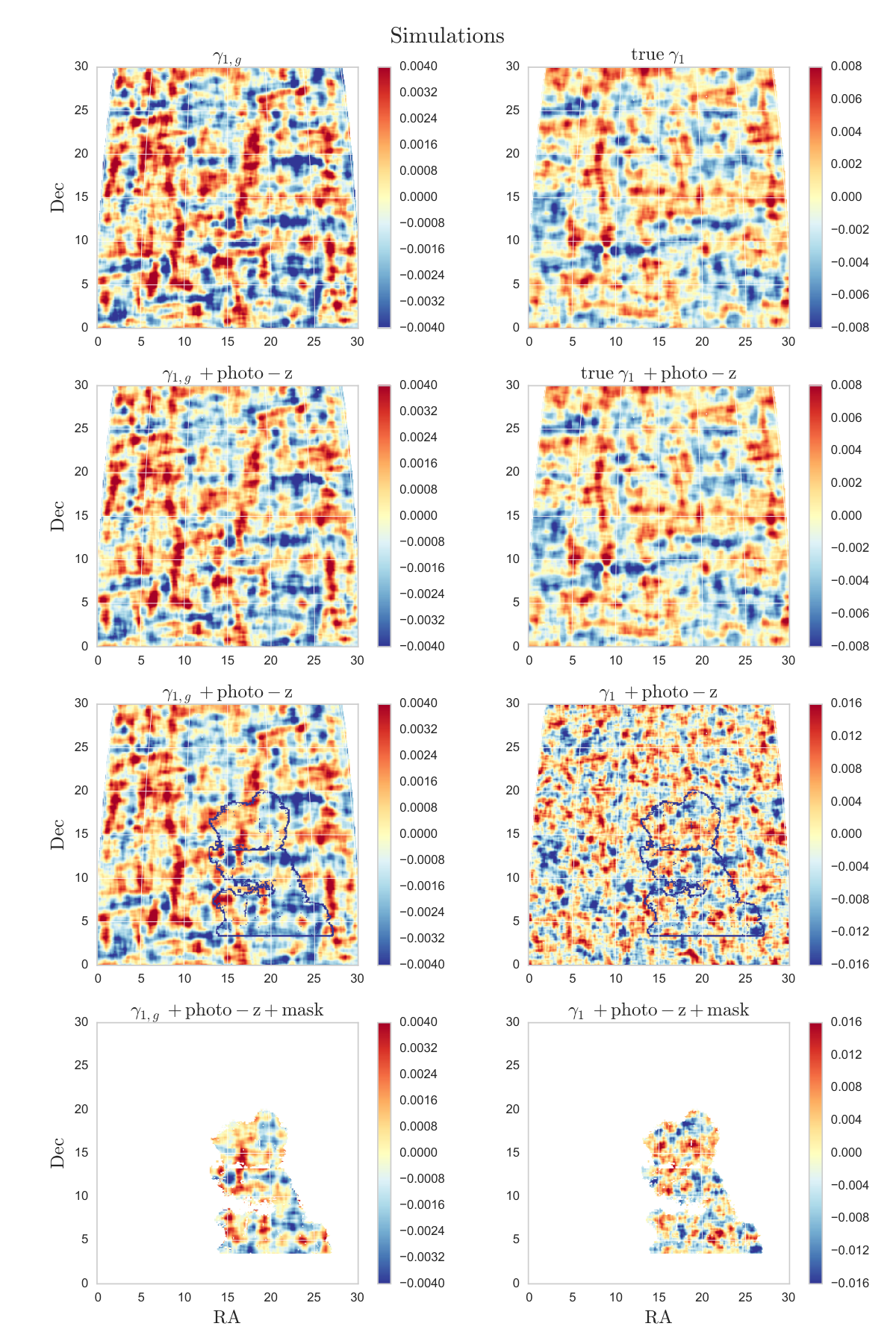
4.3 Simulation tests
Following the procedure outlined above, we present here the result of the redshift-dependent galaxy bias measurements from the MICE simulation. We start from an ideal setup in the simulations that is very close to that used in Paper I and gradually degrade the simulations until they match our data. Below we list the series of steps we take:
- 1.
use the full area ( deg2) with the true maps
- 2.
repeat above with photo- errors included
- 3.
repeat above with shape noise included
- 4.
repeat above with SV mask applied
- 5.
repeat above with 12 different SV-like areas on the sky, and vary the shape noise 100 times for each
Figure 3 illustrates an example of how the and maps degrade over these tests. The left column shows the maps while the right column shows the maps. Note that the color bars on the upper (lower) two maps in the right panel are 2 (4) times higher compared to the left column. This is to accommodate for the large change in scales on the right arising from shape noise in the maps. The first row corresponds to (i) above, and we can visually see the correspondence of some structures between the two maps. Note that the map only contributes to part of the map, which is the reason that we do not expect even the true and maps to agree perfectly. The second row shows the map with photo- errors included, corresponding to the step (ii). We find that the real structures in the maps are smoothed by the photo- uncertainties, lowering the amplitude of the map. The smoothing from the photo- is more visible in the map, since the map probes an integrated effect and is less affected by photo- errors. The third row shows what happens when shape noise is included, which corresponds to the step (iii) above. We find the structures in the map becomes barely visible in the presence of noise, with the amplitude much higher than the noiseless case as expected. The bottom row corresponds to the step (iv) above, where the SV mask is applied to both maps. For the map this is merely a decrease in the area. But for the map, this also affects the conversion from to , causing edge effects in the map which are visible in the bottom-left map in Figure 3. Step (v) is achieved by moving the mask around and drawing different random realizations of shape noise for the source galaxies.
With all maps generated, we then calculate the redshift-dependent galaxy bias following Eqn. 23 and Eqn. 24 for each of the steps from (i) to (v). In Figure 4 we show the result for the different stages, overlaid with the bias from the 2PCF measurement described in Paper I. In step (i), our measurements recover the 2PCF estimates, confirming the results in Paper I, that we can indeed measure the redshift-dependent bias using this method under appropriate settings. Our error bars are smaller than that in Paper I, which is due to the fact that we have combined measurements from several source bins, and that we estimate inverse-bias instead of bias directly. Since the only difference between this test and the test in Paper I is the inclusion of the KS conversion, we have also shown that the KS conversion in the noiseless case does not introduce significant problems in our measurements. The error bars on the highest redshift bin is large due to the small number of source and lens galaxies. In step (ii), we introduce photo- errors. We find that the photo- errors do not affect our measurements within the measurement uncertainties. In step (iii), the error bars increase due to the presence of shape noise. In (iv), we apply the SV mask, making the result much noisier due to the smaller area. We repeat this step on 12 different SV-like areas in a larger (3090 deg2) simulation area and vary the shape noise realisation 100 times for each area. The orange points in Figure 4 shows the average measurement and JK error bars of these 1,200 simulations. We find that albeit the large uncertainties, our method indeed gives an unbiased estimation of the redshift-dependent of bias which is consistent with the 2PCF estimations. In (v), we account for the additional uncertainty in our measurements due to cosmic variance. The red points are the same as the orange points, except that the error bars are estimated from the standard deviation of the 1,200 measurements in the simulations. We find that the contribution to the uncertainties from cosmic variance can be important especially at low redshift.
With the series of simulation tests above, we have shown that our measurement method itself is well grounded, but the presence of measurement effects and noise can introduces large uncertainties in the results. In the next section, we continue with the same measurement on DES SV data and will use the full simulation covariance derived in this section for the final fitting process. We believe the simulation covariance matrix captures the dominant sources of uncertainties in the problem.
| Lens redshift () | ||||
| This work (ngmix+Skynet) | ||||
| This work (im3shape+Skynet) | 1.210.25 | 1.120.24 | 0.900.19 | 0.910.28 |
| This work (ngmix+TPZ) | 1.230.23 | 1.070.18 | 1.390.40 | 1.290.44 |
| This work (ngmix+BPZ) | 0.840.11 | 1.00 0.16 | 1.130.26 | 0.950.24 |
| Crocce et al. (2016) | 1.07 0.08 | 1.240.04 | 1.340.05 | 1.560.03 |
| Giannantonio et al. (2016) | 0.57 0.25 | 0.910.22 | 0.680.28 | 1.020.31 |

4.4 Redshift-dependent galaxy bias of DES SV data
We now continue to measure redshift-dependent galaxy bias with the DES SV data using the same procedure as in the simulations. Figure 5 shows some examples of the maps. The right-most panel shows the map at redshift bin , while the rest of the maps are the maps at different redshift bin evaluated for this map. We see the effect of the lensing kernel clearly: the left-most panel is at the peak of the lensing kernel, giving it a higher weight compared to the other lens bins. We also see correlations between maps at different redshift bins. This is a result of the photo- contamination.
In Figure 6 we show the galaxy bias measurement for our magnitude-limited galaxy sample from DES SV together with two other independent measurements with the same galaxy sample (discussed in 5). We have excluded the highest redshift bin since with only a small number of source galaxies, the constraining power from lensing in that bin is very weak. The black data points show the measurement and uncertainty estimated from this work, with a best-fit linear model of: . The error bars between the redshift bins are correlated, and has been taken into account during the fit. Table 2 summarizes the results.
As discussed earlier, our method becomes much less constraining going to higher redshift, as the source galaxies become sparse. This is manifested in the increasingly large error bars going to high redshifts. Here we only performed a simple linear fit to the data given the large uncertainties in our measurements. In the future, one could extend to explore more physically motivated galaxy bias models (Matarrese et al., 1997; Clerkin et al., 2015).
Compared with A12, our data set is approximately 105 times larger, but with a (source) galaxy number density 11.6 times lower. This yields roughly times lower statistical uncertainty in our measurement. Our sample occupies a volume slightly larger than the sample in A12. Note, however, that due to photo- uncertainties and the high shape noise per unit area, we expect a slightly higher level of systematic uncertainty in our measurement. Since in A12, the emphasis was not on measuring linear bias, one should take caution in comparing directly our measurement with A12. But we note that the large uncertainties at and the weak constraints on the redshift evolution in the galaxy bias is also seen in A12. To give competitive constraints on the redshift evolution, higher redshift source planes would be needed.
4.5 Other systematics test
In 4.3, we have checked for various forms of systematic effects coming from the KS conversion, finite area, complicated mask geometry, and photo- errors. Here we perform three additional tests. First, we check that the cross-correlation between the B-mode shear and is small. Next, we check that using the second DES shear pipeline, im3shape gives consistent answers with that from ngmix. Finally, we check that using two other photo- codes also give consistent results. These three tests show that there are no significant systematic errors in our measurements.
4.5.1 B-mode test
Lensing B-mode refers to the divergent-free piece of the lensing field, which is zero in an ideal, noiseless scenario. As a result, B-mode is one of the measures for systematic effects in the data. In Jarvis et al. (2015), a large suite of tests have been carried out to ensure that the shear measurements have lower level of systematic uncertainties compared to the statistical uncertainties. Nevertheless, here we test in specific the B-mode statistics relevant to our measurements.
We construct a field by rotating the shear measurements in our data by 45 degrees, giving:
| (32) |
Substituting into in our galaxy bias calculation (Eqn. 21) gives an analogous measurement to , which we will refer to as . Since we expect not to correlate well with , would ideally go to zero. In Figure 7, we show all the measurements using both shear component and all lens-source combinations. We see that all the data points are consistent with zero at the 1–2 level, assuring that the B-modes in the shear measurements are mostly consistent with noise. We also show the weighted mean of all the data points and the corresponding B-mode measurements from one of the simulation used in 4.3 (iv). We see that the level and scatter in the data is compatible with that in the simulations.
4.5.2 im3shape test
As described in 3.3, two independent shear catalogs from DES SV were constructed. Here, we perform the same measurement in our main analysis using the im3shape catalog. The im3shape catalog contains less galaxies, thus the measurements are slightly noisier. The resulting redshift-dependent galaxy measurements are shown in Table 2 and are overall slightly higher than the ngmix measurements, and there is almost no constraining power on the evolution. The best-fit linear bias model is: , which is consistent with the ngmix measurements at the 1 level. The B-modes (not shown here) are similar to Figure 7.
4.5.3 Photo- test
As mentioned in 3.1, several photo- catalogs were generated for the DES SV data set and shown in Bonnett et al. (2015) to meet the required precision and accuracy for the SV data. All above analyzes were carried out with the Skynet photo- catalog. Here we perform the exact same analysis using the other two catalogs: BPZ and TPZ. In specific, to be consistent with the other DES SV analyzes (Becker et al., 2015; The Dark Energy Survey Collaboration et al., 2015), we keep the tomographic bins unchanged (binned by Skynet mean redshift), but use the from the different photo- codes to calculate . The lensing or galaxy maps themselves remain unchanged.
Table 2 lists the results from the different photo- catalogs. Since Skynet and TPZ are both machine learning codes and respond to systematic effects in a similar fashion, while BPZ is a template fitting code, we can thus view the difference between the results from BPZ and the others as a rough measure of the potential systematic uncertainty in our photo- algorithm (Bonnett et al., 2015, see also discussion in), which is shown here to be within the error bars.
5 Comparison with other measurements
The redshift-dependent galaxy bias has been measured on the same data set using other approaches. Here we compare our result with two other measurements – galaxy clustering (Crocce et al., 2016, hereafter C16) and cross-correlation of galaxies and CMB lensing (Giannantonio et al., 2016, hereafter G16).We note that both these analyzes assumed the most recent Planck cosmological parameters (Planck Collaboration et al., 2014), which is slightly different from our assumptions (see 3.5). But since our measurement depends very weakly on the assumption of cosmological parameters (as discussed in 2.4), the stronger cosmology dependencies come from the cosmological parameters assumed in C16 and G16, which are known well within our measurement uncertainties. We also note that the results we quote in Table 2 are based on the photo- code TPZ, which means our redshift binning is not completely identical to theirs.
5.1 Bias measurement from galaxy clustering
In C16, galaxy bias was estimated through the ratio between the projected galaxy angular correlation function (2PCF) in a given redshift bin and an analytical dark matter angular correlation function predicted at the same redshift. The latter includes both linear and nonlinear dark matter clustering derived from CAMB (Lewis et al., 2000) assuming a set of cosmological parameters. In C16, a flat CDM+ cosmological model based on Planck 2013 + WMAP polarization + ACT/SPT + BAO was used. The results in C16 as listed in Table 2 were shown to be consistent with the independent measurement from the CFHTLS (Coupon et al., 2012).
Compared to C16, our work aims to measure directly the local galaxy bias (Eqn. 1) instead of the galaxy bias defined through the 2PCF (Eqn. 2). Although the two measurements agree in the linear regime where this work is based on, comparing the measurements on smaller scales will provide further insight to these galaxy bias models. Our method is less sensitive to assumptions of cosmological parameters compared to the 2PCF method. In particular, it does not depend strongly on , which breaks the degeneracy between and the measured galaxy bias in other measurement methods. Finally, since our measurement is a cross-correlation method (compared to C16, an auto-correlation method), it suffers less from systematic effects that only contaminate either the lens or the source sample. On the other hand, however, lensing measurements are intrinsically noisy and the conversion between shear and convergence is not well behaved in the presence of noise and complicated masking. In addition, we only considered a one-point estimate (zero-lag correlation), which contains less information compared to the full 2PCF functions. All these effects result in much less constraining power in our measurements.
As shown in Figure 6 and listed in Table 2, our measurements and C16 agree very well except for the redshift bin (slightly more than 1 discrepancy). We note, however, both C16 and our work may not have included the complete allocation of systematic errors (especially those coming from the photo- uncertainties), which could introduce some of the discrepancies.
5.2 Bias measurement from cross-correlation of galaxies and CMB lensing
In G16, galaxy bias is estimated by the ratio between the galaxy-CMB convergence cross-correlation and an analytical prediction of the dark matter-CMB convergence cross-correlation, both calculated through the 2PCF (and also in harmonic space through the power spectrum). Since the lensing efficiency kernel of the CMB is very broad and the CMB lensing maps are typically noisy, this method has less constraining power than C16. However, by using an independent external data, the CMB lensing maps from the South Pole Telescope and the Planck satellite, this measurement serves as a good cross check for possible systematic effects in the DES data.
In calculating the theoretical dark matter-CMB convergence cross-correlation, G16 also assumed a fixed cosmology and derived all predictions using CAMB. The - degeneracy is thus also present in their analysis. We note, however, that one could apply our method to the CMB lensing data and avoid this dependency. In our framework, the CMB lensing plane will serve as an additional source plane at redshift 1100. We defer this option to future work.
The results from G16 are shown in Figure 6 and listed in Table 2. These results come from the ratio between the measured and the predicted power spectrum, which suffers less from non-linear effects compared to the measurement in real space (2PCF). We find that G16 is systematically lower than our measurement at the 1-2 level for all redshift bins. G16 also has more constraining power at high redshift compared to our results, as expected. Possible reasons for the discrepancy at low redshift include systematic errors (in e.g. the photo- estimation) that are not included in either C16, G16 or this work. In addition, the redshift bins are significantly covariant, making the overall discrepancy less significant. Finally, the scales used in the three studies are slightly different. We refer the readers to G16 for more discussion of this discrepancy.
6 Conclusion
In this paper, we present a measurement of redshift-dependent bias using a novel technique of cross-correlating the weak lensing shear maps and the galaxy density maps. The method serves as an alternative measurement to the more conventional techniques such as 2-point galaxy clustering, and is relatively insensitive to the assumed cosmological parameters. The method was first developed in Amara et al. (2012) and later tested more rigorously with simulations in a companion paper (Pujol et al., 2016, Paper I). Here we extend the method and apply it on wide-field photometric galaxy survey data for the first time. We measure the galaxy bias for a magnitude-limited galaxy sample in the Dark Energy Survey (DES) Science Verification (SV) data.
Following from Paper I, we carry out a series of simulation tests which incorporate step-by-step realistic effects in our data including shape noise, photo- errors and masking. In each step, we investigate the errors introduced in our estimation of galaxy bias. We find that shape noise and cosmic variance are the main sources of uncertainties, while the photo- affects the measurements in a predictable way if the characteristics of the photo- uncertainties are well understood. As the measurement itself is very noisy, simulation tests where we know the “truth” provide a good anchor for building the analysis pipeline.
In our main analysis, we measure the galaxy bias with a magnitude-limited galaxy sample in 4 tomographic redshift bins to be (), (), (), and (). Measurements from higher redshifts are too noisy to be constraining. The best-fit linear model gives: . The results are consistent between different shear and photo- catalogs.
The galaxy bias of this same galaxy sample has also been measured with two other techniques described in Crocce et al. (2016) and Giannantonio et al. (2016). The three measurements agree at the 1–2 level at all four redshift bins, though the results from Giannantonio et al. (2016) are systematically lower than our measurements. We note that our method is more constraining at low redshift regions where there are more source galaxies behind the lens galaxies. As pointed out in Amara et al. (2012), to constrain the evolution of galaxy bias, our current data set may not be optimal. A more efficient configuration would be combining a wide, shallow data set with a narrow, deep field. We plan on exploring these possibilities in the future. The main uncertainty in this work comes from the combined effect of masking, shape noise and cosmic variance. However, as we demonstrated with simulations, moving to the larger sky coverage of the first and second year of DES data would reduce this effect significantly.
We have demonstrated the feasibility and validity of our method for measuring galaxy bias on a wide-field photometric data set. Looking forward to the first and second year of DES data (2,000 square degrees and magnitude shallower), we expect to explore a variety of other topics using this method with the increased statistical power. For example, the same measurement could be carried out on different subsamples of lens galaxies (in magnitude, color, galaxy type etc.) and gain insight into the different clustering properties for different galaxy populations. Also, one can extend the measurement into the non-linear regime and measure the scale-dependencies of the galaxy bias. Finally, it would be interesting to compare the measurement from the 2PCF method and our method (which is a measure of local bias) on different scales to further understand the connections between the two galaxy bias models.
Acknowledgement
We thank Marc Manera, Donnacha Kirk, Andrina Nicola, Sebastian Seehars for useful discussion and feedback. CC, AA, AR and TK are supported by the Swiss National Science Foundation grants 200021-149442 and 200021-143906. AP was supported by beca FI and 2009-SGR-1398 from Generalitat de Catalunya and project AYA2012-39620 from MICINN. JZ and SB acknowledge support from the European Research Council in the form of a Starting Grant with number 240672.
We are grateful for the extraordinary contributions of our CTIO colleagues and the DECam Construction, Commissioning and Science Verification teams in achieving the excellent instrument and telescope conditions that have made this work possible. The success of this project also relies critically on the expertise and dedication of the DES Data Management group.
Funding for the DES Projects has been provided by the U.S. Department of Energy, the U.S. National Science Foundation, the Ministry of Science and Education of Spain, the Science and Technology Facilities Council of the United Kingdom, the Higher Education Funding Council for England, the National Center for Supercomputing Applications at the University of Illinois at Urbana-Champaign, the Kavli Institute of Cosmological Physics at the University of Chicago, the Center for Cosmology and Astro-Particle Physics at the Ohio State University, the Mitchell Institute for Fundamental Physics and Astronomy at Texas A&M University, Financiadora de Estudos e Projetos, Fundação Carlos Chagas Filho de Amparo à Pesquisa do Estado do Rio de Janeiro, Conselho Nacional de Desenvolvimento Científico e Tecnológico and the Ministério da Ciência, Tecnologia e Inovação, the Deutsche Forschungsgemeinschaft and the Collaborating Institutions in the Dark Energy Survey.
The Collaborating Institutions are Argonne National Laboratory, the University of California at Santa Cruz, the University of Cambridge, Centro de Investigaciones Energéticas, Medioambientales y Tecnológicas-Madrid, the University of Chicago, University College London, the DES-Brazil Consortium, the University of Edinburgh, the Eidgenössische Technische Hochschule (ETH) Zürich, Fermi National Accelerator Laboratory, the University of Illinois at Urbana-Champaign, the Institut de Ciències de l’Espai (IEEC/CSIC), the Institut de Física d’Altes Energies, Lawrence Berkeley National Laboratory, the Ludwig-Maximilians Universität München and the associated Excellence Cluster Universe, the University of Michigan, the National Optical Astronomy Observatory, the University of Nottingham, The Ohio State University, the University of Pennsylvania, the University of Portsmouth, SLAC National Accelerator Laboratory, Stanford University, the University of Sussex, and Texas A&M University.
The DES data management system is supported by the National Science Foundation under Grant Number AST-1138766. The DES participants from Spanish institutions are partially supported by MINECO under grants AYA2012-39559, ESP2013-48274, FPA2013-47986, and Centro de Excelencia Severo Ochoa SEV-2012-0234. Research leading to these results has received funding from the European Research Council under the European Union’s Seventh Framework Programme (FP7/2007-2013) including ERC grant agreements 240672, 291329, and 306478.
References
- Amara et al. (2012) Amara A., et al., 2012, MNRAS, 424, 553
- Bartelmann & Schneider (2001) Bartelmann M., Schneider P., 2001, Physics Reports, 340, 291
- Becker et al. (2015) Becker M. R., et al., 2015, preprint, (arXiv:1507.05598)
- Benítez (2000) Benítez N., 2000, ApJ, 536, 571
- Bertin (2006) Bertin E., 2006, in Gabriel C., Arviset C., Ponz D., Enrique S., eds, Astronomical Society of the Pacific Conference Series Vol. 351, Astronomical Data Analysis Software and Systems XV. p. 112
- Bertin (2011) Bertin E., 2011, in Evans I. N., Accomazzi A., Mink D. J., Rots A. H., eds, Astronomical Society of the Pacific Conference Series Vol. 442, Astronomical Data Analysis Software and Systems XX. p. 435
- Bertin & Arnouts (1996) Bertin E., Arnouts S., 1996, A&AS, 117, 393
- Bertin et al. (2002) Bertin E., Mellier Y., Radovich M., Missonnier G., Didelon P., Morin B., 2002, in Bohlender D. A., Durand D., Handley T. H., eds, Astronomical Society of the Pacific Conference Series Vol. 281, Astronomical Data Analysis Software and Systems XI. p. 228
- Blake et al. (2008) Blake C., Collister A., Lahav O., 2008, MNRAS, 385, 1257
- Blanton (2000) Blanton M., 2000, ApJ, 544, 63
- Bonnett et al. (2015) Bonnett C., et al., 2015, preprint, (arXiv:1507.05909)
- Carrasco Kind & Brunner (2013) Carrasco Kind M., Brunner R. J., 2013, MNRAS, 432, 1483
- Carrasco Kind & Brunner (2014) Carrasco Kind M., Brunner R. J., 2014, MNRAS, 442, 3380
- Carretero et al. (2015) Carretero J., Castander F. J., Gaztañaga E., Crocce M., Fosalba P., 2015, MNRAS, 447, 646
- Chang et al. (2015) Chang C., et al., 2015, Physical Review Letters, 115, 051301
- Clerkin et al. (2015) Clerkin L., Kirk D., Lahav O., Abdalla F. B., Gaztañaga E., 2015, MNRAS, 448, 1389
- Coupon et al. (2012) Coupon J., et al., 2012, A&A, 542, A5
- Cresswell & Percival (2009) Cresswell J. G., Percival W. J., 2009, MNRAS, 392, 682
- Crocce et al. (2015) Crocce M., Castander F. J., Gaztañaga E., Fosalba P., Carretero J., 2015, MNRAS, 453, 1513
- Crocce et al. (2016) Crocce M., et al., 2016, MNRAS, 455, 4301
- Desai et al. (2012) Desai S., et al., 2012, ApJ, 757, 83
- Eriksen & Gaztanaga (2015) Eriksen M., Gaztanaga E., 2015, preprint, (arXiv:1508.00035)
- Flaugher et al. (2015) Flaugher B., et al., 2015, AJ, 150, 150
- Fosalba et al. (2015a) Fosalba P., Gaztañaga E., Castander F. J., Crocce M., 2015a, MNRAS, 447, 1319
- Fosalba et al. (2015b) Fosalba P., Crocce M., Gaztañaga E., Castander F. J., 2015b, MNRAS, 448, 2987
- Giannantonio et al. (2016) Giannantonio T., et al., 2016, MNRAS, 456, 3213
- Graff et al. (2014) Graff P., Feroz F., Hobson M. P., Lasenby A., 2014, MNRAS, 441, 1741
- Hartlap et al. (2007) Hartlap J., Simon P., Schneider P., 2007, A&A, 464, 399
- Jarvis et al. (2015) Jarvis M., et al., 2015, preprint, (arXiv:1507.05603)
- Jullo et al. (2012) Jullo E., et al., 2012, ApJ, 750, 37
- Kaiser (1984) Kaiser N., 1984, ApJ, 284, L9
- Kaiser & Squires (1993) Kaiser N., Squires G., 1993, ApJ, 404, 441
- Leistedt et al. (2015) Leistedt B., et al., 2015, preprint, (arXiv:1507.05647)
- Lewis et al. (2000) Lewis A., Challinor A., Lasenby A., 2000, ApJ, 538, 473
- MacQueen (1967) MacQueen J., 1967, in Proceedings of the Fifth Berkeley Symposium on Mathematical Statistics and Probability, Volume 1: Statistics. University of California Press, Berkeley, Calif., pp 281–297, http://projecteuclid.org/euclid.bsmsp/1200512992
- Mandelbaum et al. (2013) Mandelbaum R., Slosar A., Baldauf T., Seljak U., Hirata C. M., Nakajima R., Reyes R., Smith R. E., 2013, MNRAS, 432, 1544
- Manera & Gaztañaga (2011) Manera M., Gaztañaga E., 2011, MNRAS, 415, 383
- Matarrese et al. (1997) Matarrese S., Coles P., Lucchin F., Moscardini L., 1997, MNRAS, 286, 115
- Mohr et al. (2012) Mohr J. J., et al., 2012. (arXiv:1207.3189), doi:10.1117/12.926785
- Ngeow et al. (2006) Ngeow C., et al., 2006. p. 23 (arXiv:astro-ph/0608246), doi:10.1117/12.671017
- Planck Collaboration et al. (2014) Planck Collaboration et al., 2014, A&A, 571, A16
- Pujol et al. (2016) Pujol A., et al., 2016, preprint, (arXiv:1601.00160)
- Rykoff et al. (2015) Rykoff E. S., Rozo E., Keisler R., 2015, preprint, (arXiv:1509.00870)
- Sánchez et al. (2014) Sánchez C., et al., 2014, MNRAS, 445, 1482
- Schneider (1998) Schneider P., 1998, ApJ, 498, 43
- Sevilla et al. (2011) Sevilla I., et al., 2011, preprint, (arXiv:1109.6741)
- Sheldon (2014) Sheldon E. S., 2014, MNRAS, 444, L25
- Simon et al. (2007) Simon P., Hetterscheidt M., Schirmer M., Erben T., Schneider P., Wolf C., Meisenheimer K., 2007, A&A, 461, 861
- Simon et al. (2009) Simon P., Hetterscheidt M., Wolf C., Meisenheimer K., Hildebrandt H., Schneider P., Schirmer M., Erben T., 2009, MNRAS, 398, 807
- Swanson et al. (2008) Swanson M. E. C., Tegmark M., Blanton M., Zehavi I., 2008, MNRAS, 385, 1635
- The Dark Energy Survey Collaboration et al. (2015) The Dark Energy Survey Collaboration et al., 2015, preprint, (arXiv:1507.05552)
- Vikram et al. (2015) Vikram V., et al., 2015, Phys.Rev.D, 92, 022006
- Wild et al. (2005) Wild V., et al., 2005, MNRAS, 356, 247
- Zehavi et al. (2011) Zehavi I., et al., 2011, ApJ, 736, 59
- Zuntz et al. (2013) Zuntz J., Kacprzak T., Voigt L., Hirsch M., Rowe B., Bridle S., 2013, MNRAS, 434, 1604
Appendix A Choice of estimator
In our main analysis, we use the inverse-galaxy bias as our main estimator instead of estimating galaxy bias directly. In this appendix we show the effect of using as the estimator. The origin of the difference comes from the fact that when combining the multiple measurements in the same lens bin, we use the least-square formalism Eqn. 23, which relies on the covariance matrix estimated through JK resampling. This covariance matrix can become ill-behaved depending on the estimator used. In our case, the denominator of (the inverse of Eqn. 21) can become close to zero, which makes the inversion of the covariance matrix unstable. We find that this introduces a bias in our final result, which will need to be calibrated.
In Figure 8 we show the equivalent of Figure 4 using as an estimator instead of . As the distribution of estimated through the simulations have large outliers, we exclude simulations with bias estimates below 0 and above 5. We find that the main difference between Figure 4 and Figure 8 is in the orange and red points, where all the observational effects are included. For the less noisy scenarios (i)(ii) and (iii), the change is very minor. This is because the effect is more manifested when the measurements are noisy. The final (red) points in Figure 8 is biased from the “truth” by due to the matrix inversion discussed above.
Once we calibrate from these simulations and apply it to the data measurements, we have Figure 9, which is the equivalent of Figure 6 but using as an estimator instead of . We find that after taking into account the bias derived from Figure 4, the final measurements from the data is still consistent with our main analysis in Figure 6. Nevertheless, as using relies heavily of the quality of the simulations and the outlier-rejection described above is not entirely objective, we choose to use the estimator instead.
Affiliations
1Department of Physics, ETH Zurich, Wolfgang-Pauli-Strasse 16, CH-8093 Zurich, Switzerland
2Institut de Ciències de l’Espai, IEEC-CSIC, Campus UAB, Facultat de Ciències, Torre C5 par-2, 08193 Bellaterra, Barcelona, Spain
3Institute of Cosmology & Gravitation, University of Portsmouth, Portsmouth, PO1 3FX, UK
4Department of Physics, Stanford University, 382 Via Pueblo Mall, Stanford, CA 94305, USA
5Kavli Institute for Particle Astrophysics & Cosmology, P. O. Box 2450, Stanford University, Stanford, CA 94305, USA
6Institut de Física d’Altes Energies, Universitat Autònoma de Barcelona, E-08193 Bellaterra, Barcelona, Spain
7Institute of Astronomy, University of Cambridge, Madingley Road, Cambridge CB3 0HA, UK
8Kavli Institute for Cosmology, University of Cambridge, Madingley Road, Cambridge CB3 0HA, UK
9Centre for Theoretical Cosmology, DAMTP, University of Cambridge, Wilberforce Road, Cambridge CB3 0WA, UK
10Department of Physics and Astronomy, University of Pennsylvania, Philadelphia, PA 19104, USA
11Center for Cosmology and Astro-Particle Physics, The Ohio State University, Columbus, OH 43210, USA
12Brookhaven National Laboratory, Bldg 510, Upton, NY 11973, USA
13Jodrell Bank Center for Astrophysics, School of Physics and Astronomy, University of Manchester, Oxford Road, Manchester, M13 9PL, UK
14Argonne National Laboratory, 9700 South Cass Avenue, Lemont, IL 60439, USA
15Cerro Tololo Inter-American Observatory, National Optical Astronomy Observatory, Casilla 603, La Serena, Chile
16Department of Physics & Astronomy, University College London, Gower Street, London, WC1E 6BT, UK
17Department of Physics and Electronics, Rhodes University, PO Box 94, Grahamstown, 6140, South Africa
18Fermi National Accelerator Laboratory, P. O. Box 500, Batavia, IL 60510, USA
19CNRS, UMR 7095, Institut d’Astrophysique de Paris, F-75014, Paris, France
20Sorbonne Universités, UPMC Univ Paris 06, UMR 7095, Institut d’Astrophysique de Paris, F-75014, Paris, France
21SLAC National Accelerator Laboratory, Menlo Park, CA 94025, USA
22Laboratório Interinstitucional de e-Astronomia - LIneA, Rua Gal. José Cristino 77, Rio de Janeiro, RJ - 20921-400, Brazil
23Observatório Nacional, Rua Gal. José Cristino 77, Rio de Janeiro, RJ - 20921-400, Brazil
24Department of Physics, University of Illinois, 1110 W. Green St., Urbana, IL 61801, USA
25National Center for Supercomputing Applications, 1205 West Clark St., Urbana, IL 61801, USA
26School of Physics and Astronomy, University of Southampton, Southampton, SO17 1BJ, UK
27Faculty of Physics, Ludwig-Maximilians-Universitaet, Scheinerstr. 1, 81679 Muenchen, Germany
28Excellence Cluster Universe, Boltzmannstr. 2, 85748 Garching, Germany
29Jet Propulsion Laboratory, California Institute of Technology, 4800 Oak Grove Dr., Pasadena, CA 91109, USA
30Department of Astronomy, University of Michigan, Ann Arbor, MI 48109, USA
31Department of Physics, University of Michigan, Ann Arbor, MI 48109, USA
32Kavli Institute for Cosmological Physics, University of Chicago, Chicago, IL 60637, USA
33Department of Astronomy, University of California, Berkeley, 501 Campbell Hall, Berkeley, CA 94720, USA
34Lawrence Berkeley National Laboratory, 1 Cyclotron Road, Berkeley, CA 94720, USA
35Max Planck Institute for Extraterrestrial Physics, Giessenbachstrasse, 85748 Garching, Germany
36Department of Physics, The Ohio State University, Columbus, OH 43210, USA
37Australian Astronomical Observatory, North Ryde, NSW 2113, Australia
38George P. and Cynthia Woods Mitchell Institute for Fundamental Physics and Astronomy, and Department of Physics and Astronomy,
Texas A&M University, College Station, TX 77843, USA
39Departamento de Física Matemática, Instituto de Física, Universidade de São Paulo, CP 66318, CEP 05314-970, São Paulo, SP, Brazil
40Department of Astrophysical Sciences, Princeton University, Peyton Hall, Princeton, NJ 08544, USA
41Institució Catalana de Recerca i Estudis Avançats, E-08010 Barcelona, Spain
42Department of Physics and Astronomy, Pevensey Building, University of Sussex, Brighton, BN1 9QH, UK
43Centro de Investigaciones Energéticas, Medioambientales y Tecnológicas (CIEMAT), Madrid, Spain