Detecting quasinormal modes of binary black hole mergers with second-generation gravitational-wave detectors
Abstract
Recent population synthesis simulations of Pop III stars suggest that the event rate of coalescence of – binary black holes can be high enough for the detection by the second generation gravitational wave detectors. The frequencies of chirp signal as well as quasinormal modes are near the best sensitivity of these detectors so that it would be possible to confirm Einstein’s general relativity. Using the WKB method, we suggest that for the typical value of spin parameter from numerical relativity results of the coalescence of binary black holes, the strong gravity of the black hole space-time at around the radius , which is just times the event horizon radius, would be confirmed as predicted by general relativity. The expected event rate with the signal-to-noise ratio needed for the determination of the quasinormal mode frequency with the meaningful accuracy is – where and are the peak value of the Pop III star formation rate and the fraction of binaries, respectively. As for the possible optical counter part, if the merged black hole of mass is in the interstellar matter with and the proper motion of black hole is , the luminosity is which can be detected up to , for example, by Subaru-HSC and LSST with the limiting magnitude 26.
pacs
04.30.-w,04.25.-g,04.70.-sI Introduction
The second generation gravitational wave detectors such as Advanced LIGO (aLIGO) [1], Advanced Virgo (AdV) [2], and KAGRA [3, 4] are now about to reach the observable mean distance of Mpc for the chirp signal of neutron star (NS)–NS binaries. Among them, aLIGO is now operating with the range of – Mpc from September 18, 2015 to mid-January in 2016 [5]. One of the most important targets is NS–NS mergers which might be associated with Short Gamma Ray Bursts (SGRBs). There are three methods to determine the expected event rate of NS–NS mergers. The first one is to use the observed NS–NS binaries. Kim, Kalogera and Lorimer [6] performed Monte Carlo simulations using the already existing pulsar surveys. Assuming the pulsar distribution function in our galaxy, the luminosity function of pulsars and pulsar beaming factors, they concluded that the event rate is for aLIGO, AdV and KAGRA adopting their model 1 although there is a factor of 38 difference in the rate among their 27 models. Kalogera et al. [7] corrected the rate since the new double pulsar PSR J0737-3039 was found. The new rate becomes using their model 6 which predicts about three times larger rate than that of model 1. Kalogera et al. [7] corrected the error in their simulations which reduced the rate to . The latest expected event rate by Kim et al. [8] is at confidence level, adopting their model 6. This further reduction mainly comes from the new beaming factor correction obtained from the observations of PSR J0737-3039.
The second method is to use the observed event rate of SGRBs assuming that the SGRB is NS–NS and/or NS–black hole (BH) mergers. Here, we should note that no NS–BH binary has been observed as a pulsar binary. According to Fong et al. [9], the number of SGRBs with the confirmed redshift by Swift and HETE-2 is at most 20 or so. However, BATSE on CGRO [10] found SGRBs between 1990 and 2000 without the information of redshift . To determine the redshifts of these SGRBs, the – relation for SGRBs found by Tsutsui et al. [11] can be used. Here, and mean the peak energy of the photon and the peak luminosity of the SGRB, respectively. The empirical relation is given by
| (1) |
Using the observed flux ) with the luminosity distance , and the peak energy of the photon , we can determine the redshift . Yonetoku et al. [12] used the 72 bright BATSE SGRBs for the analysis since we need many photons to determine . They obtained the minimum event rate of SGRBs as , with the observational input that the mean jet opening angle of SGRBs is . This corresponds to the minimum event rate of if SGRBs are NS–NS mergers, while the minimum event rate is if SGRBs are the NS–BH (of mass 10) mergers. In this analysis, because they do not use NS–NS binary data, even if only of SGRBs are NS–BH binaries, the minimum event rate becomes (see also Refs. [13, 14, 15, 16] for the related works).
The third method is the theoretical population synthesis method. A recent paper by Dominik et al. [17] includes the chemical evolution effect of galaxies with metalicity from to , that is, from Pop I to Pop II stars (see Ref. [18] for a formation of massive stellar BH-BH binaries). The resulting event rates depend on various parameters, assumptions on the binary interaction, detectors and the number of detectors, to yield – for NS–NS mergers and – for NS–BH mergers (see also Ref. [19] for predictions for the event rates of compact binary coalescences).
In the case of BH–BH binaries, there is no definite candidate so that the theoretical population synthesis is the only method to predict the rate. In this regard, Pop III stars are important. Pop III stars are the first stars in our universe without the heavy metal, that is, their envelope consists of H and He only. While Pop I stars are similar to our sun with heavy elements in mass with atomic number larger than carbon. Pop II stars are low metal stars with heavy elements in mass. Observationally Pop I and Pop II stars suffer mass loss due to the absorption of photons at the metal lines. This means that because Pop III stars do not lose their mass, massive BHs are more likely to be formed.
Recently Kinugawa et al. [20, 21] showed by using the population synthesis code that the typical chirp mass of the Pop III binary BHs is with the total mass of . This means that comparable mass ratio binary BHs are typical. Here, we note three important facts. The first one is that Pop III stars were formed at , while a sizable fraction of BH–BH binaries merge today since the merger time is proportional to the fourth power of the initial orbital separation. The second one is that the typical mass of Pop III stars had been considered to be , while Hosokawa et al. [22] showed that the UV photons from the central star evaporate the accretion disk so that the mass is around . The third one is that Pop III star of mass ends its life not as a red giant but as a blue giant, according to the evolution calculations of Pop III stars by Marigo et al. [23]. This means that since the mass loss due to the binary interaction is small, the formation of – binary BHs is expected. Kinugawa et al. [20, 21] performed the population synthesis of binary Pop III stars for 14 models and obtained – for aLIGO [1], AdV [2] and KAGRA [3, 4] where and are the peak value of the Pop III star formation rate and the fraction of binaries, respectively. We should emphasize here that the factor difference among various models exists like in Refs. [6, 7, 8] for NS–NS merger rates. In the cases of Pop I and Pop II, Dominik et al. [17] showed that the typical chirp mass of BH–BH binary is smaller than that in the Pop III case and the event rate ranges from to .
As shown by Kanda et al. [24], the chirp signal and the quasinormal mode (QNM) frequency of – binary BHs are in the best sensitivity band of aLIGO, AdV and KAGRA. Therefore, there is a good chance to observe the QNM which will exhibit the strong gravity space-time near the event horizon to confirm Einstein’s general relativity. To confirm the expected signal of the QNM, the threshold signal-to-noise ratio (SNR) which is usually used for the detection, is not enough. For this confirmation, Nakano, Tanaka and Nakamura [25] have shown that SNR events of – Pop III BH–BH merger are the appropriate target. Then, for the Pop III case, the event rate for SNR becomes – (see Ref. [26] for a comparison of evolutionary predictions with initial and forthcoming LIGO/Virgo upper limits, and related works [27, 28]). It is noted that there are various proposals for the formation of heavy BH binaries [29, 30, 31].
What we can say definitely when the QNM is confirmed to exist at the expected frequency, is the main theme of this paper. Since QNMs are obtained under the ingoing and outgoing wave conditions at the event horizon and the spatial infinity, respectively, the most optimistic statement is that all the space-time of a Kerr BH is tested. However, even if the event horizon might be absent, fuzzy or blocked by the firewall (see, e.g., Refs. [32, 33, 34, 35]), we will observe something similar to the QNMs predicted by general relativity (see Refs. [36, 37]). In this paper, we would like to ask what we can say more robustly.
This paper is organized as follows. In Sec. II, we compare the Regge-Wheeler and Zerilli potentials [38, 39] and the WKB analysis of the QNM for the Schwarzschild BH. In Sec. III, we use the Sasaki-Nakamura equation [40, 41, 42] for the Kerr BH, while in Sec. IV, we use the (Chandrasekhar and) Detweiler equation [43]. Section V is devoted to discussions. In the analysis of QNMs in this paper, we focus only on the () mode since BH binary merger simulations indicate that the () QNM is dominant (see e.g., Ref. [44]). We use the geometric unit system, where in this paper.
II Regge-Wheeler and Zerilli Equation
For the Schwarzschild BH case with mass , the metric is given by
| (2) |
We may use the Regge-Wheeler and Zerilli equations [38, 39] to obtain the gauge invariant perturbation. The Regge-Wheeler (odd parity) / Zerilli (even parity) function satisfies the Regge-Wheeler or Zerilli equation,
| (3) |
where and the potentials are given as
| (4) | |||||
| (5) | |||||
where is the index of the spherical harmonics . The potential for the even parity is slightly complicated, but according to Ref. [45], both and are written in a unified manner as
| (6) | |||||
| (7) |
where the upper and lower signs are for the even and odd parities, respectively. Then, the Regge-Wheeler and Zerilli equations become
| (8) |
For the even parity, we can have the same differential equation as the odd parity, i.e., the modified function satisfies
| (9) |
To do so, we consider the transformation of the wave function,
| (10) | |||||
| (11) |
where
| (12) |
This is called the Chandrasekhar transformation. Therefore, the same QNMs are obtained in the Regge-Wheeler and Zerilli equations.
To study BH QNMs, the WKB approximation has been used frequently [46]. While the full analysis of the QNMs gives the same frequencies for the odd and even parity perturbations, we have different results in the leading order WKB analysis [47] (see Sec. III for a brief summary). In the WKB approximation, the QNM frequency is determined by the information around the peak of the potential. The peak of is obtained explicitly as
| (13) |
On the other hand, we calculate the peak location of in the large expansion because of the complicated potential, and derive
| (14) |
This should be compared with in the large expansion,
| (15) |
which shows that the difference between and is . For example, this difference for the mode is numerically shown in
| (16) |
Therefore, although the peak location slightly depends on which potential we adopt, this can be a good estimator to discuss where the QNMs are emitted.
III Sasaki-Nakamura Equation
For the Kerr BH case, the metric is given by
| (17) |
where and are the mass and the spin parameter, respectively, and . Teukolsky [48] showed that the gravitational perturbation is separable and the radial equation is given by
| (18) |
where is the source and
| (19) |
with
| (20) |
and and come from and the spin-weighted spheroidal function , respectively. Here, a prime means the derivative with respect to . The source term diverges as for a particle falling into the Kerr BH, and the potential takes the long range nature. Therefore, Sasaki and Nakamura [40, 41, 42] proposed a new equation with the convergent source term and the short range potential as the followings.
Specifying two functions and , we can define various variables as
| (21) | |||||
| (22) | |||||
| (23) | |||||
| (24) | |||||
| (25) | |||||
| (26) |
Then, we have the wave equation as
| (27) |
where
| (28) |
We adopt and defined by
| (29) | |||||
| (30) |
where
| (31) | |||||
| (32) |
Then, defining a new variable by , we have
| (33) |
where
| (34) |
A remarkable feature of is that the potential becomes the Regge-Wheeler potential for .
Schutz and Will [47] derived the QNM for the Regge-Wheeler potential by using the WKB method. The essence of their method is to approximate by the expansion near its peak at as
| (35) |
where . Then the fundamental () QNM frequency is expressed as
| (36) |
They have found that for the QNM frequency of the mode, the errors of the real () and the imaginary () parts are and , respectively, compared with the numerical results of Chandrasekhar and Detweiler [49].
Since one needs to impose the ingoing and outgoing boundary conditions at the event horizon and the spatial infinity, respectively, to derive QNM frequencies, one might say that the existence of the event horizon is confirmed if the QNM of a Schwarzschild BH is detected. However, the WKB method by Schutz and Will [47] suggests that what we can conservatively claim is that the space-time of a Schwarzschild BH around is tested since both real and imaginary parts of the QNM frequency are determined by the value of and its curvature at .
What we want to do is to establish a similar statement for the Kerr BH case. Since numerical relativity simulations for binary BHs [50, 51, 52] suggest that the final Kerr parameter after the merger of equal-mass, nonspinning BHs is about (see Ref. [53] for the latest remnant spin formula), instead of the Regge-Wheeler potential we need to discuss the Kerr case with the potential .
An important difference of the Kerr case is that the potential becomes complex even if one uses the real potential for the real frequency such as Detweiler [43]. Since the separation constant of the radial and angular Teukolsky equations depends on , which is complex in the QNM calculation, the above potential becomes complex. Therefore, there is no advantage to use the real potential in our approach, and the complex nature of for is not an essential drawback. Our purpose is not to determine the QNM frequencies correctly by the WKB method since there is a good numerical method to determine them by Leaver [54]. Our interest is in what we can claim conservatively when the QNM of a Kerr BH is detected by the second generation gravitational wave detectors, aLIGO, AdV and KAGRA. That is, our goal is to find a similar physical picture as Schutz and Will [47] did for the Schwarzschild case, i.e., the BH space-time near can be confirmed by the QNMs of a BH with .
We therefore substitute the numerical value of the QNM frequency for the Kerr BH case by Ref. [55] (see useful Berti’s “Ringdown” website [56]) as well as the dependence of up to the sixth order by Ref. [57] into the potential . It is noted that the error between the fitting function of lambda and the exact numerical value is less than for the QNM frequency. The left panel of Fig. 1 shows the values of the potential, , and with ) as a function of in the case of . We see that is close to and contribution of is small so that we can identify the critical radius , i.e., with the peak of . For the case with ), it is still reasonable to use the peak as shown in the right panel of Fig. 1. Since we cannot apply the standard WKB approximation for double peaks shown in the right panel of Fig. 1, the estimation for in the current analysis is not mathematically appropriate. For smaller values of , the contribution of is much smaller than the case.


Therefore, it would not be a bad approximation to expand near the peak of (or ) as Schutz and Will [47] did for the Schwarzschild case as
| (37) |
For definiteness, we choose to evaluate the above expression at the peak of , and we denote that real-valued radius as . Then, we can estimate the QNM frequency by
| (38) |
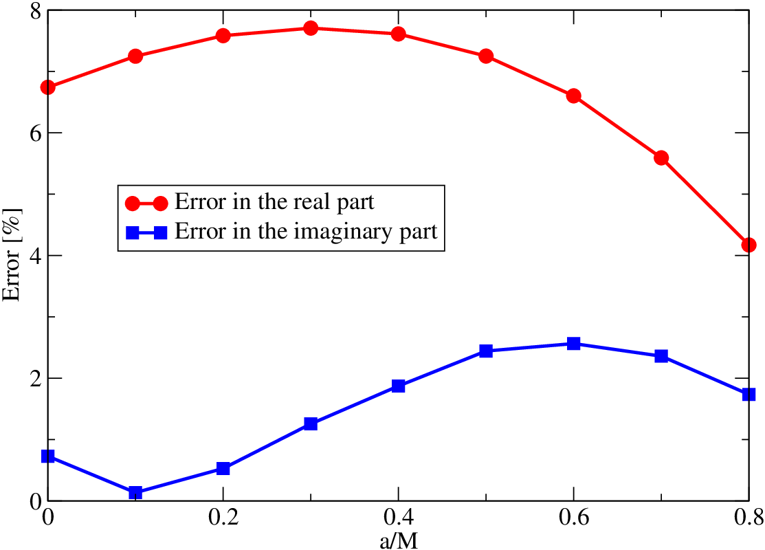
This approximation will be worse when becomes large. The location of the maximum of the absolute value of the potential , and the real and imaginary parts of the QNM frequencies with () are shown in Figs. 2 and 3, respectively. In Fig. 4, we present the errors in the frequencies. We can say that our approximate method reproduces the QNM frequencies within accuracy which supports our approximation. It is noted that fine structures in the imaginary part of Figs. 2 and 3 are due to the complicated behavior of the potential with respect to . A local maximum arises in for , and has two peaks for .


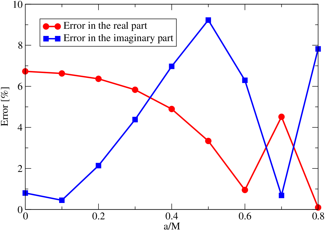
In the above analysis, assuming the smallness of , we have derived by finding the peak of . But to use Eq. (37) exactly, it is necessary to find for in the complex plane. Then, we may mention the effective peak radius by the real part of because the imaginary part of is small. This also supports the argument to use the real derived from the peak of . Some brief analysis is summarized in Appendix A, and we find a good agreement between the peak location of and the real part of of .
As a result, we may say that if the QNM with is detected with an accuracy of , the BH space-time around which is times the event horizon, is confirmed. Here, we know that we cannot localize gravitational waves within a small region less than its wavelength. Since the wavelength of the QNM that we are concerned is , the origin of the QNM is also necessarily extended to a similar amount. The extension should be measured in the coordinate. The non-local nature of gravitational waves is reflected by the appearance of the second derivative of the potential in the expression of Eq. (38). The local value of the second derivative at the peak can be varied by arranging the transformation. However, we would have to pay the expense that the potential will tend to take more wavy shape and possibly possess multiple extrema.
From the Pop III star population synthesis, the expected event rate is – where and are the peak value of the Pop III star formation rate and the fraction of binaries, respectively [21]. Since the range of the above rate is not derived from the statistical treatment and the minimum rate of is obtained from the most unlikely model, there will be a good chance to observe the QNM with SNR .
IV Chandrasekhar and Detweiler Equation
Chandrasekhar and Detweiler developed various transformations in the radial Teukolsky equation (see, e.g, Ref. [59] and related references therein). Here, we use the notation in Appendix B of Ref. [43].
The two functions and in Eq. (21) are now
| (39) | |||||
| (40) |
where is the same as the one in the previous section while , and
| (41) | |||||
| (42) | |||||
| (43) | |||||
| (44) |
There is a typo 11 1 Although we do not use Eq. (B8) of Ref. [43], there should be a typo, and it reads as (45) Here, the definition of in the above equation has the inverse signature of Eq. (20) due to . in Eq. (B19) of Ref. [43], i.e., in should be as the above equation. We have confirmed that and in Eqs. (40) give a constant in Eq. (22), i.e., a constant in Eq. (11) of Ref. [43]. In the above equations, we have
| (46) | |||||
| (47) | |||||
| (48) |
The differential equation for becomes
| (49) |
where and is calculated from Eq. (15) with Eq. (13) of Ref. [43] (or from Eq. (26) with Eqs. (24) and (25) in this paper where is identical to and , see also Eq. (27) of Ref. [60] to correct a typo in Eq. (B23) of Ref. [43]). When we adopt , the potential takes a slightly simpler expression, given in Eq. (B24) of Ref. [43] as
| (51) | |||||
As noted in Sec. III, the above potential is the real potential for the real frequency . However, since the QNM frequencies are complex, becomes complex in our analysis.
When we take the positive (negative) signature for in Eq. (48), the potential becomes the Zerilli (Regge-Wheeler ) potential in the Schwarzschild limit. As shown in Fig. 5 for the case, the best potential with ) in order to apply the WKB approximation is obtained by choosing the negative signature for in Eq. (47) and the positive signature for in Eq. (48). In this case, the extremum is clearly unique. We call this situation the () case. As a reference, we also present the case in the right panel of Fig. 5.


Seidel and Iyer [60] found that the positive signature of is the best choice for the mode in the case with the negative signature of , i.e., the () case, for example, in Fig. 5. In their analysis of Ref. [60], a higher order WKB approximation was employed (see also a Kokkotas’s work [61]). They expand their real potential , i.e., the () case for real frequency and which is the value of such that is maximized as
| (52) | |||||
| (53) |
where () and () are the potential for the Schwarzschild case and the value of such that is maximized, respectively. Then, they solve
| (54) |
to determine . To calculate the () QNM frequency, they solve
| (55) |
where the function can be derived by their Eq. (2). After obtaining a complex QNM frequency, becomes complex. This is the reason why we do not adopt their method since our purpose is not to obtain the accurate QNM frequency (see e.g., Ref. [62] for inaccuracy of the WKB method), but to establish the physical picture that the QNM brings us information around the peak radius .
In our analysis for the () case, the QNM frequency is calculated by
| (56) |
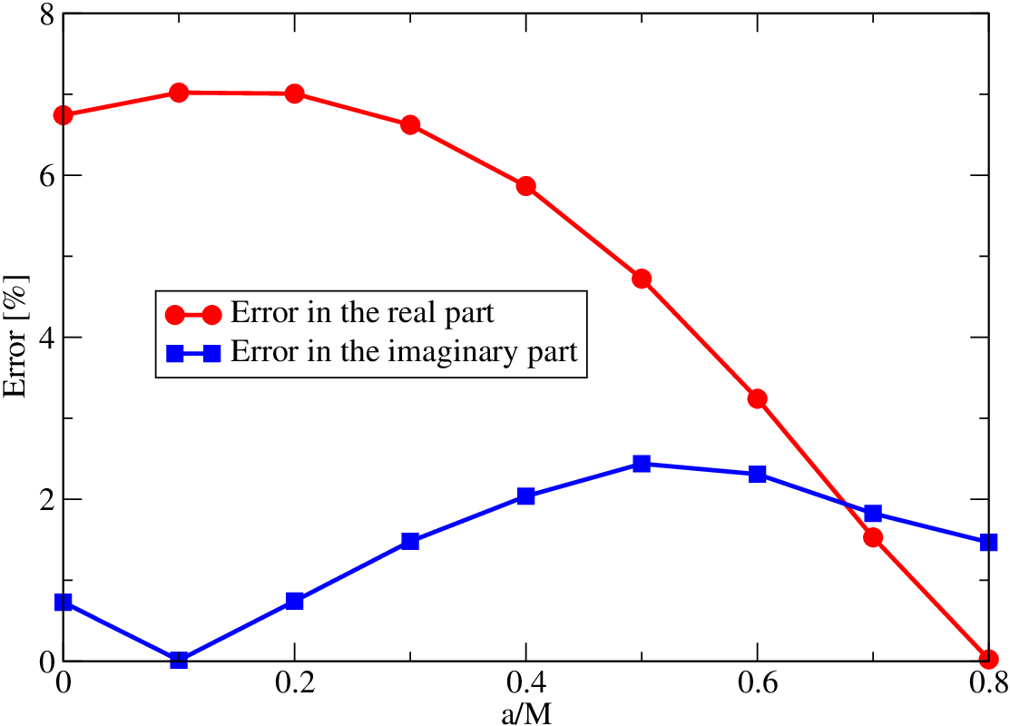
Again, this is an approximation because we adopt the peak of as , and the approximation will be worse when becomes large. The location of the maximum of the absolute value of the potential with () (see Fig. 6 for the smallness of the imaginary part of the potential), and the real and imaginary parts of the QNM frequencies are shown in Figs. 7 and 8, respectively. Since the contribution of the imaginary part is small, we use the peak location of as in the WKB approximation. In Fig. 9, we show the errors in the frequencies. From Fig. 7, we see that for the peak of with ) is , i.e., , which is similar to the case in Sec. III. Fig. 9 shows that the error of the QNM frequencies is , which is also similar to the case presented in Sec. III.


V Discussions
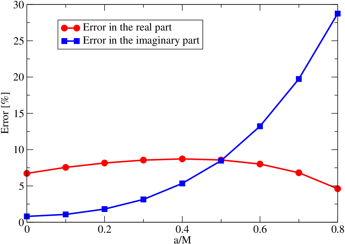
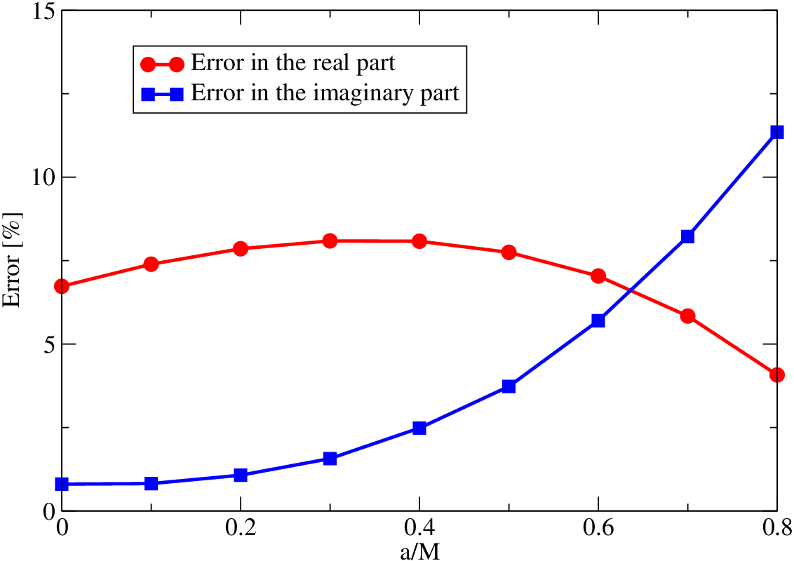
In the case of the Chandrasekhar and Detweiler equation, we have used , i.e, the () case. It might be interesting to see the peak locations and the QNM frequencies in the WKB analysis for the other cases. Fig. 10 shows the location of the maximum of the absolute value of the potential with ) for the , and cases. As seen in Fig. 5, the peak location depends on the choice of the signatures in and . We find that the , and cases do not give a better result for the QNM frequency (see Fig. 11) than the case in applying the WKB approximation of Eq. (56). The relative errors in the evaluation of the QNM frequencies compared with the exact value are presented in Fig. 12. In particular, the imaginary part of the QNM frequency deviates from the exact one substantially for . This is not mainly due to the crude approximation for adopted in this paper. Even if we use corresponding to the complex root of , the errors necessarily grow for a larger value of . (Although the estimate of the QNM frequency changes, the tendency that the error increases in that regime is not altered.) The main cause of the error would be due to the appearance of the second root of near the real axis of , which we can imagine for , , and cases for as the appearance of double extrema or wavy shape in the plot of . The appearance of the second root is confirmed also by direct calculation. By contrast, does not seem to suffer from any significant contribution from other roots up to .


Our purpose of the current study is to establish the picture that the QNMs are approximately originating from the peak location of the potential. The peak location varies depending on the choice of the potential, but the variance is not very large as seen in Figs. 2, 7 and 10. Furthermore, we find that the estimate of the QNM frequencies by using , and cases is better than that in the and cases. If the cases that give worse estimate of the QNM frequencies, i.e., the and cases are excluded, the variance of the peak location becomes even smaller.
In the high frequency regime the real and imaginary parts of the QNM frequencies are thought to be related to the orbital frequency of the light ring orbit and the Lyapunov exponent of the perturbation around it, respectively (see Refs. [63, 64, 65, 66, 67, 68] for the related works and a useful lecture note [69]). In Figs. 2, 7 and 10 we display the inner light ring radius on the equatorial plane as a reference. From this comparison, the peak location is found to be well approximated by the inner light ring radius, especially for , and cases. This fact suggests that even for the lowest order QNM with the light ring radius is a good approximation for the region that is responsible for generation of QNMs (see pioneer works in Refs. [70, 71]).
One may think that QNM frequencies depend on the boundary condition imposed in the very vicinity of the event horizon, and therefore modification to general relativity through the change of the boundary condition may lead to some observable effect. However, we find it unlikely to find the effect as modified QNM frequencies, from the following consideration. Suppose that complete reflection boundary condition is imposed at a distance in the proper distance from the event horizon. This radius is, roughly speaking, , in the coordinate, and hence it takes time of before a wave completes a round trip between and this hypothetical reflection boundary. If we choose the Planck length for as expected by the stringy modification such as the firewall, this time scale for the round trip becomes as long as , which is much longer than the time scale of the decay of QNMs, which is typically . Therefore, we find that the effect of the modified boundary condition will not appear as a measurable shift of the QNM frequencies in near future, even if we assume an extreme situation such as a complete reflection. However, the effect of the modification of the boundary condition may arise in a different manner or in a very accurate future measurement of the QNM frequencies as an observable signature (see Refs. [36, 37]). We may come back to this issue in our future publication.
In Ref. [25] we discussed binaries such that form a BH with . In the expected noise curve of KAGRA [bKAGRA, VRSE(D) configuration] presented in Ref. [72], the parameter estimation (1) errors for the real and imaginary parts with SNR are and , respectively, by using the Fisher analysis (see, e.g., Refs. [73, 74, 75, 76] for the QNM gravitational wave data analysis). Therefore, we concluded that we have a good chance to confirm the existence of black hole formed as a result of binary merger.
When we have at hand not just a feature of black hole candidates but a clear evidence for the existence of BHs by the QNM observation, we will have to wait sitting on a gold mine, if we cannot find a clue to carry out further research. The breakthrough might be brought by the detection of the electro-magnetic counterpart. Let us consider a merged BH with mass moving with the velocity in the interstellar gas with the number density . Then, the accretion rate is estimated as
| (57) | |||||
| (58) | |||||
| (59) |
where is the mass of the proton and efficiency of the available gravitational energy at the innermost stable circular orbit (ISCO) for is assumed. The luminosity is comparable to the Eddington luminosity of star, i.e., . If this energy is emitted mainly in the X-ray, the wide field X-ray telescope such as ISS lobster can observe up to about Mpc since the limiting flux is [77]. While if the energy is emitted mainly in the optical band, it can be detected up to Mpc by Subaru-HSC [78] and LSST [79] with the limiting magnitude 26 for example. It should be noted that, since the sky location of this gravitational wave source is for the event with SNR, this area can be covered by one or a few shots with Subaru-HSC [78] and LSST [79].
The mass formula of the Kerr BH with the gravitational mass and the angular momentum is given by
| (60) |
where is the irreducible mass of the Kerr BH (see, e.g., Ref. [80]). Expressing , we have
| (61) |
where . Eq. (61) is solved as
| (62) |
Therefore, the maximum energy available by the extraction of all the angular momentum is given by
| (63) |
For , becomes
| (64) |
This energy is so huge that the possible electromagnetic counter part of Pop III – mergers exists. Therefore, one might think that the Blandford-Znajek (BZ) [81] luminosity might be much larger. Now the rotational velocity at ISCO is . Assuming the equipartition of the ram pressure energy to the magnetic field energy at ISCO, the magnetic strength is roughly estimated as
| (65) | |||||
| (66) |
According to Eq. (A6) of Penna et al. [82], the BZ power derived from the magnetic flux of their Eq. (A4) and the angular velocity of the event horizon as
| (67) | |||||
| (68) |
which is smaller than the accretion energy unfortunately. Here, we recovered and in the above equation for convenience. We need a certain process to increase the magnetic field strength near the event horizon to liberate the huge energy shown in Eq. (64) to be visible in electromagnetic radiation to identify the position as well as the strong gravity space-time near the event horizon of the BH since the mean distance to Pop III BH merger is , i.e., Gpc in the luminosity distance.
Finally we like to mention that the current scenario that SGRBs are identified with NS–NS and/or NS–BH mergers does not have any smoking gun so far. For example, it is usually claimed that no SGRB accompanied the supernova explosion, and hence SGRBs are different from Long GRBs (LGRBs). However, there are at least two LGRBs without the supernova association [83]. Only the detection of gravitational waves from SGRBs can be the smoking gun of this scenario. Concerning this, before 1997 almost all GRB scientists except for a few people including Paczynski believed that GRBs are not at a cosmological distance but within at most in the halo of our galaxy from various suggestions, without any smoking gun. The cosmological redshift found in the afterglow of GRB 970508 was the smoking gun of the cosmological origin of GRBs to force more than 2000 papers useless. As one of the counter theories against the current scenario, there is, for example, an unified model of LGRB, SGRB, XRR (X-ray Rich GRB) and XRF (X-Ray Flash) (see, e.g., Yamazaki, Ioka and Nakamura [84]). Even if the current scenario of SGRBs turns out to be incorrect unexpectedly, Pop III BH–BH binary mergers discussed in this paper would be another plausible candidates of the important sources of gravitational waves to search the strong gravity space-time near the event horizon of the BH of mass .
Acknowledgements.
We thank T. Sakamoto for a careful reading of this manuscript, and for helpful comments. We would also like to appreciate the anonymous referee for valuable comments. This work was supported by MEXT Grant-in-Aid for Scientific Research on Innovative Areas, “New Developments in Astrophysics Through Multi-Messenger Observations of Gravitational Wave Sources”, No. 24103006 (TN, HN, TT) and by the Grant-in-Aid from the Ministry of Education, Culture, Sports, Science and Technology (MEXT) of Japan No. 15H02087 (TN, TT).Appendix A Another estimation
In this appendix, we summarize the effective peak radius derived from the real part of the radius which satisfies . Fig. 13 shows the radii obtained from various potentials. Although it is difficult to understand the jump in the radius between and in the analysis the maximum of the absolute value of the potential , we find the reason from the calculation of in the complex plane. For , we have a solution . On the other hand, we have two solutions for , and . Here, the peak location of for corresponds to the latter solution. It is also noted that the imaginary part of the solution for is always an order of magnitude smaller than the real part in the current analysis between and , and we find a good agreement between the peak location of and the real part of of , comparing Figs. 2, 7 and 10 with Fig. 13.

References
- [1] J. Aasi et al. [LIGO Scientific Collaboration], Class. Quant. Grav. 32, 074001 (2015) [arXiv:1411.4547 [gr-qc]].
- [2] F. Acernese et al. [VIRGO Collaboration], Class. Quant. Grav. 32, 024001 (2015) [arXiv:1408.3978 [gr-qc]].
- [3] K. Somiya [KAGRA Collaboration], Class. Quant. Grav. 29, 124007 (2012) [arXiv:1111.7185 [gr-qc]].
- [4] Y. Aso et al. [KAGRA Collaboration], Phys. Rev. D 88, 043007 (2013) [arXiv:1306.6747 [gr-qc]].
- [5] https://www.advancedligo.mit.edu/nov_2015_news.html
- [6] C. Kim, V. Kalogera and D. R. Lorimer, Astrophys. J. 584, 985 (2003) [astro-ph/0207408].
- [7] V. Kalogera et al., Astrophys. J. 601, L179 (2004) [Astrophys. J. 614, L137 (2004)] [astro-ph/0312101].
- [8] C. Kim, B. B. P. Perera and M. A. McLaughlin, Mon. Not. Roy. Astron. Soc. 448, 928 (2015) [arXiv:1308.4676 [astro-ph.SR]].
- [9] W. F. Fong et al., Astrophys. J. 769, 56 (2013) [arXiv:1302.3221 [astro-ph.HE]].
- [10] http://heasarc.gsfc.nasa.gov/docs/cgro/index.html
- [11] R. Tsutsui, D. Yonetoku, T. Nakamura, K. Takahashi and Y. Morihara, Mon. Not. Roy. Astron. Soc. 431, 1398 (2013) [arXiv:1208.0429 [astro-ph.HE]].
- [12] D. Yonetoku, T. Nakamura, K. Takahashi, A. Toyanago and T. Sawano, Astrophys. J. 789, 65 (2014) [arXiv:1402.5463 [astro-ph.HE]].
- [13] C. E. Petrillo, A. Dietz and M. Cavaglia, Astrophys. J. 767, 140 (2013) [arXiv:1202.0804 [astro-ph.CO]].
- [14] S. Nissanke, M. Kasliwal and A. Georgieva, Astrophys. J. 767, 124 (2013) [arXiv:1210.6362 [astro-ph.HE]].
- [15] K. Siellez, M. Boer and B. Gendre, Mon. Not. Roy. Astron. Soc. 437, 649 (2014) [arXiv:1310.2106 [astro-ph.HE]].
- [16] T. Regimbau, K. Siellez, D. Meacher, B. Gendre and M. Boer, Astrophys. J. 799, 69 (2015) [arXiv:1410.2739 [astro-ph.HE]].
- [17] M. Dominik et al., Astrophys. J. 806, 263 (2015) [arXiv:1405.7016 [astro-ph.HE]].
- [18] K. Belczynski, A. Buonanno, M. Cantiello, C. L. Fryer, D. E. Holz, I. Mandel, M. C. Miller and M. Walczak, Astrophys. J. 789, 120 (2014) [arXiv:1403.0677 [astro-ph.HE]].
- [19] J. Abadie et al. [LIGO Scientific and VIRGO Collaborations], Class. Quant. Grav. 27, 173001 (2010) [arXiv:1003.2480 [astro-ph.HE]].
- [20] T. Kinugawa, K. Inayoshi, K. Hotokezaka, D. Nakauchi and T. Nakamura, Mon. Not. Roy. Astron. Soc. 442, 2963 (2014) [arXiv:1402.6672 [astro-ph.HE]].
- [21] T. Kinugawa, A. Miyamoto, N. Kanda and T. Nakamura, Mon. Not. Roy. Astron. Soc. 456, 1093 (2016) [arXiv:1505.06962 [astro-ph.SR]].
- [22] T. Hosokawa, K. Omukai, N. Yoshida and H. W. Yorke, Science 334, 1250 (2011) [arXiv:1111.3649 [astro-ph.CO]].
- [23] P. Marigo, L. Girardi, C. Chiosi and P. R. Wood, Astron. Astrophys. 371, 152 (2001) [astro-ph/0102253].
- [24] N. Kanda [LCGT Collaboration], arXiv:1112.3092 [astro-ph.IM].
- [25] H. Nakano, T. Tanaka and T. Nakamura, Phys. Rev. D 92, 064003 (2015) [arXiv:1506.00560 [astro-ph.HE]].
- [26] K. Belczynski, S. Repetto, D. Holz, R. O’Shaughnessy, T. Bulik, E. Berti, C. Fryer and M. Dominik, arXiv:1510.04615 [astro-ph.HE].
- [27] M. Dominik, K. Belczynski, C. Fryer, D. Holz, E. Berti, T. Bulik, I. Mandel and R. O’Shaughnessy, Astrophys. J. 759, 52 (2012) [arXiv:1202.4901 [astro-ph.HE]].
- [28] M. Dominik, K. Belczynski, C. Fryer, D. E. Holz, E. Berti, T. Bulik, I. Mandel and R. O’Shaughnessy, Astrophys. J. 779, 72 (2013) [arXiv:1308.1546 [astro-ph.HE]].
- [29] P. Amaro-Seoane and X. Chen, arXiv:1512.04897 [astro-ph.CO].
- [30] I. Mandel and S. E. de Mink, arXiv:1601.00007 [astro-ph.HE].
- [31] P. Marchant, N. Langer, P. Podsiadlowski, T. Tauris and T. Moriya, arXiv:1601.03718 [astro-ph.SR].
- [32] P. O. Mazur and E. Mottola, gr-qc/0109035.
- [33] S. D. Mathur, Fortsch. Phys. 53, 793 (2005) [hep-th/0502050].
- [34] S. L. Braunstein, S. Pirandola and K, Życzkowski, Phys. Rev. Lett. 110, 101301 (2013) [arXiv:0907.1190 [quant-ph]].
- [35] A. Almheiri, D. Marolf, J. Polchinski and J. Sully, JHEP 1302, 062 (2013) [arXiv:1207.3123 [hep-th]].
- [36] T. Damour and S. N. Solodukhin, Phys. Rev. D 76, 024016 (2007) [arXiv:0704.2667 [gr-qc]].
- [37] E. Barausse, V. Cardoso and P. Pani, Phys. Rev. D 89, 104059 (2014) [arXiv:1404.7149 [gr-qc]].
- [38] T. Regge and J. A. Wheeler, Phys. Rev. 108, 1063 (1957).
- [39] F. J. Zerilli, Phys. Rev. D 2, 2141 (1970).
- [40] M. Sasaki and T. Nakamura, Phys. Lett. A 89, 68 (1982).
- [41] M. Sasaki and T. Nakamura, Prog. Theor. Phys. 67, 1788 (1982).
- [42] T. Nakamura and M. Sasaki, Phys. Lett. A 89, 185 (1982).
- [43] S. L. Detweiler, Proc. Roy. Soc. Lond. A 352, 381 (1977).
- [44] L. London, D. Shoemaker and J. Healy, Phys. Rev. D 90, 124032 (2014) [arXiv:1404.3197 [gr-qc]].
- [45] S. Chandrasekhar, The mathematical theory of black holes, OXFORD, UK: CLARENDON (1985).
- [46] B. Mashhoon, Phys. Rev. D 31, 290 (1985).
- [47] B. F. Schutz and C. M. Will, Astrophys. J. 291, L33 (1985).
- [48] S. A. Teukolsky, Astrophys. J. 185, 635 (1973).
- [49] S. Chandrasekhar and S. L. Detweiler, Proc. Roy. Soc. Lond. A 344, 441 (1975).
- [50] F. Pretorius, Phys. Rev. Lett. 95, 121101 (2005) [gr-qc/0507014].
- [51] M. Campanelli, C. O. Lousto, P. Marronetti and Y. Zlochower, Phys. Rev. Lett. 96, 111101 (2006) [gr-qc/0511048].
- [52] J. G. Baker, J. Centrella, D. I. Choi, M. Koppitz and J. van Meter, Phys. Rev. Lett. 96, 111102 (2006) [gr-qc/0511103].
- [53] J. Healy, C. O. Lousto and Y. Zlochower, Phys. Rev. D 90, 104004 (2014) [arXiv:1406.7295 [gr-qc]].
- [54] E. W. Leaver, Proc. Roy. Soc. Lond. A 402, 285 (1985).
- [55] E. Berti, V. Cardoso and C. M. Will, Phys. Rev. D 73, 064030 (2006) [gr-qc/0512160].
- [56] http://www.phy.olemiss.edu/~berti/ringdown/
- [57] W. H. Press and S. A. Teukolsky, Astrophys. J. 185, 649 (1973).
- [58] J. M. Bardeen, W. H. Press and S. A. Teukolsky, Astrophys. J. 178, 347 (1972).
- [59] S. Chandrasekhar and S. L. Detweiler, Proc. Roy. Soc. Lond. A 350, 165 (1976).
- [60] E. Seidel and S. Iyer, Phys. Rev. D 41, 374 (1990).
- [61] K. D. Kokkotas, Nuovo Cim. B 108, 991 (1993).
- [62] E. Berti, V. Cardoso and A. O. Starinets, Class. Quant. Grav. 26, 163001 (2009) [arXiv:0905.2975 [gr-qc]].
- [63] V. Cardoso, A. S. Miranda, E. Berti, H. Witek and V. T. Zanchin, Phys. Rev. D 79, 064016 (2009) [arXiv:0812.1806 [hep-th]].
- [64] S. R. Dolan and A. C. Ottewill, Class. Quant. Grav. 26, 225003 (2009) [arXiv:0908.0329 [gr-qc]].
- [65] S. R. Dolan, Phys. Rev. D 82, 104003 (2010) [arXiv:1007.5097 [gr-qc]].
- [66] H. Yang, D. A. Nichols, F. Zhang, A. Zimmerman, Z. Zhang and Y. Chen, Phys. Rev. D 86, 104006 (2012) [arXiv:1207.4253 [gr-qc]].
- [67] H. Yang, F. Zhang, A. Zimmerman, D. A. Nichols, E. Berti and Y. Chen, Phys. Rev. D 87, 041502 (2013) [arXiv:1212.3271 [gr-qc]].
- [68] H. Yang, A. Zimmerman, A. Zengino?lu, F. Zhang, E. Berti and Y. Chen, Phys. Rev. D 88, 044047 (2013) [Phys. Rev. D 88, 044047 (2013)] [arXiv:1307.8086 [gr-qc]].
- [69] E. Berti, arXiv:1410.4481 [gr-qc].
- [70] W. H. Press, Astrophys. J. 170, L105 (1971). doi:10.1086/180849
- [71] C. J. Goebel, Astrophys. J. 172, L95 (1972).
- [72] http://gwcenter.icrr.u-tokyo.ac.jp/researcher/parameters
- [73] H. Nakano, H. Takahashi, H. Tagoshi and M. Sasaki, Phys. Rev. D 68, 102003 (2003) [gr-qc/0306082].
- [74] H. Nakano, H. Takahashi, H. Tagoshi and M. Sasaki, Prog. Theor. Phys. 111, 781 (2004) [gr-qc/0403069].
- [75] Y. Tsunesada, N. Kanda, H. Nakano, D. Tatsumi, M. Ando, M. Sasaki, H. Tagoshi and H. Takahashi, Phys. Rev. D 71, 103005 (2005) [gr-qc/0410037].
- [76] Y. Tsunesada et al. [TAMA Collaboration], Class. Quant. Grav. 22, S1129 (2005).
- [77] S. Kisaka, K. Ioka and T. Nakamura, Astrophys. J. 809, L8 (2015) [arXiv:1506.02030 [astro-ph.HE]].
- [78] http://subarutelescope.org/Projects/HSC/index.html
- [79] http://www.lsst.org/
- [80] C. W. Misner, K. S. Thorne and J. A. Wheeler, Gravitation, SAN FRANCISCO: W. H. FREEMAN AND CO. (1973).
- [81] R. D. Blandford and R. L. Znajek, Mon. Not. Roy. Astron. Soc. 179, 433 (1977).
- [82] R. F. Penna, R. Narayan and A. Sadowski, Mon. Not. Roy. Astron. Soc. 436, 3741 (2013) [arXiv:1307.4752 [astro-ph.HE]].
- [83] J. P. U. Fynbo et al., Nature 444, 1047 (2006) [astro-ph/0608313].
- [84] R. Yamazaki, K. Ioka and T. Nakamura, Astrophys. J. 607, L103 (2004) [astro-ph/0401142].