Large-scale Monte Carlo simulations for the depinning transition in Ising-type lattice models

The DRFIM is one of the simplest demonstration to study the depinning transition in the disorder media with microscopic structures and interactions. The Hamiltonian of the DRFIM can be written as

$$\mathcal{H}=-J\sum_{<ij>}S_{i}S_{j}-H\sum_{i}S_{i}-\sum_{i}h_{i}S_{i},$$

(1)

where $S_{i}=\pm 1$ is the classical Ising spin of the two-dimensional rectangle lattice with $2L\times L$, the random field $h_{i}$ is uniformly distributed within an interval $[-\Delta,\Delta]$, and $H$ is a homogeneous driving field. The initial state that spins are positive in the sublattice on the left side and negative on the right side, is used to build a perfect domain wall, also referred to as a “domain interface”, in the $y$ direction. The direction perpendicular to the domain interface is then set to the $x$ axis. Antiperiodic and periodic boundary conditions are used in $x$ and $y$ directions, respectively. To eliminate the pinning effect irrelevant for disorder, we rotate the square lattice such that the initial domain wall orients in the $(11)$ direction of the square lattice, as shown in Refs. [43, 48, 51, 54].

After preparing the initial state, a usual Monte Carlo method is adopted with standard one-spin flips in the simulations. Simply speaking, we update each spin with the following procedure. Firstly, we randomly choose a single spin $S_{i}$ in the two-dimensional lattice. The change of the total energy is then calculated after we flip the spin $S_{i}\rightarrow S_{i}^{\prime}$,

	$\displaystyle\delta E$	$\displaystyle=$	$\displaystyle\mathcal{H}(S_{i})-\mathcal{H}(S_{i}^{\prime})$		(2)
		$\displaystyle=$	$\displaystyle(S_{i}^{\prime}-S_{i})\left[-J\sum_{j}S_{j}-H-h_{i}\right].$

Only when $\delta E<0$, the flip is accepted, otherwise the spin state $S_{i}$ remains. A Monte Carlo time step (MCS) is defined by $2L^{2}$ single-spin updates. As time evolves, the domain wall moves and roughens, while the bulk, i.e., spins far away from the domain interface, keeps invariant. As shown in Fig. 1, the time evolution of the spin configuration is displayed with the black and whites squares, corresponding to $S_{i}=\pm 1$, respectively. Complicated spin structure are found nearby the domain interface, such as overhangs and islands at the time $t=1\penalty\ 000$ MCS.

According to earlier literatures [1, 38, 49], there are many different ways to define the domain interface. In this paper, we adopt a simple and popular definition based on the magnetization. Denoting a spin at site $(x,y)$ by $S_{xy}(t)$, a microscopic height function of the domain interface is introduced,

$$h(y,t)=\frac{L_{x}}{2}[m(y,t)+1],$$

(3)

where $m(y,t)$ is the linear magnetization defined as

$$m(y,t)=\frac{1}{L_{x}}\left[\sum_{x=1}^{L_{x}}S_{xy}(t)\right],$$

(4)

and $L_{x}$ is the size of the lattice in the $x$ direction. The velocity of the domain interface is then calculated as

$$v(t)=\frac{d\langle h(y,t)\rangle}{dt},$$

(5)

where $\langle\cdots\rangle$ includes both the statistical average over samples and in the $y$ direction. To depict the roughening process of the domain interface, the roughness function $\omega(t)$ and correlation function $C(r,t)$ are measured with

$$\omega^{(2)}(t)=\left\langle h(y,t)^{2}\right\rangle-\langle h(y,t)\rangle^{2},$$

(6)

and

$$C(r,t)=\left\langle h(y+r,t)h(y,t)\right\rangle-\left\langle h(y,t)\right\rangle^{2},$$

(7)

respectively. The former describes the roughening of the domain interface in the $x$ direction, and the latter reflects the growth of the spatial correlation in the $y$ direction. Moreover, the function $F(t)$ is measured as the ratio of the planar susceptibility and line susceptibility [48, 49, 50],

$$F(t)\sim[M^{(2)}(t)-M(t)^{2}]/\omega^{2}(t),$$

(8)

where $M(t)$ is the total magnetization, and $M^{(2)}(t)$ is its second moment.

In addition, other types of the quenched disorder are also considered for comparison, taking the random-bond disorder in the DBDIM as an example. The Hamiltonian of the DBDIM is

$$\mathcal{H}=-\sum_{<ij>}J_{ij}S_{i}S_{j}-H\sum_{i}S_{i},$$

(9)

where $J_{ij}=1+\varepsilon_{ij}$ denotes the nearest-neighboring coupling strength, and $\varepsilon_{ij}$ is the bond disorder following a Gaussian distribution with the mean zero and the standard deviation $\sigma$. Without loss of generality, we set $\sigma=1.5$ in the simulations as an example of the strong-disorder case.

In usual Monte Carlo simulations, we are limited to the system size $L_{x}=2L_{y}=2\penalty\ 048$ up to $t_{max}=2\penalty\ 000$ MCS for a sufficiently large sample size $N_{s}=20\penalty\ 000$ [48, 50], since all of the spins in the lattice, on average, should be chosen and updated in each MCS. However, the number of the activated spins $N(t)$ decreases quickly with the time $t$, as shown in Fig. 1. Where the activated spin is defined that each attempt of the flip will be accepted once the spin is chosen. As an example, $N(t)=68$ is obtained at $t=1\penalty\ 000$ MCS, much smaller than the total spin number $2L^{2}\approx 10^{6}$. Consequently, most of the spins are inactivated in Monte Carlo simulations. To avoid the undesirable waste of the time, the EMC algorithm is developed in this paper with the architecture:

Step $1$: Initialize the spin lattice with a perfect domain interface. The quenched disorder $h_{i}(x,y)$ is generated randomly for each site in the rectangle lattice.

Step $2$: Create a table list of the activated spins. To be specific, we search for the spins with the energy change $\delta E<0$ according to Eq. (2), and store their position information $(x,y)$ in the table list. The number of activated spins $N(t)$ is then obtained as the size of the table list.

Step $3$: Update the table list. In this table list, we randomly choose a spin, flip it with $S_{i}\rightarrow-S_{i}$, and delete its position information. Afterwards, the change of the energy $\delta E$ is respectively calculated for its four nearest-neighboring spins. If $\delta E<0$, new position information is added into the table list.

Step $4$: Increase the time of the EMC simulation to $t^{\prime}=t+1/N(t)$ MCS. Physical observable of the system including the microscopic height function $h(y,t^{\prime})$, roughness function $\omega(t^{\prime})$, and correlation function $C(r,t^{\prime})$), are then assessed.

Step $5$: Repeat the steps $3$ and $4$ until the time of the simulation $t>t_{max}$ indicating that a sample of the simulation is terminated.

Step $6$: Repeat the steps $1\sim 5$ for the statistical average over samples and realizations of the quenched disorder. The velocity of the domain interface $v(t)$ is then calculated with Eq. (5).

With the EMC algorithm, the depinning transition with lattice sizes from $L=32$ to $12\penalty\ 000$ is investigated up to $t_{max}=22\penalty\ 000$ MCS. Our main results are presented at $L=8\penalty\ 192$, much larger than $L=1\penalty\ 024$ in earlier literatures [48, 50], and simulation results at $L=12\penalty\ 000$ confirm that finite-size effects are already negligibly small. Besides, the influence of the disorder strength is also investigated, taking the uniformly distributed random field $h_{i}$ with the strength varying from $\Delta=0$ to $10$. For each set of the parameters, more than $20\penalty\ 000$ samples are performed for average. Statistical errors are estimated by dividing the total samples in three subgroups. If the fluctuation in the time direction is comparable with or larger than the statistical error, it also will be taken into account.

As the depinning transition is of second order, the short-time scaling theory [52, 53] is applicative for the time evolution of the order parameter $v(t)$. The dynamic scaling form is derived by scaling arguments with a finite lattice size $L$ and nonequilibrium spatial correlation length $\xi\sim t^{1/z}$,

$$v(t,\tau,L)=b^{-\beta/\nu}G(b^{-z}t,b^{1/\nu}\tau,b^{-1}L),$$

(10)

where $b$ denotes an arbitrary rescaling factor, $\beta$ and $\nu$ correspond to the static exponents, $z$ is the dynamic exponent, and $\tau=(H-H_{c})/H_{c}$. Setting $b\sim t^{1/z}$, the scaling form can be simplified in the short-time scaling regime with $\xi(t)\sim t^{1/z}\ll L$,

$$v(t,\tau)=t^{-\beta/\nu z}G(t^{1/\nu z}\tau).$$

(11)

Only at the transition point $\tau=0$, a power law behavior is expected,

$$v(t)\sim t^{-\beta/\nu z}.$$

(12)

The critical field $H_{c}$ is then located by searching for the best power-law behavior of $v_{{}_{M}}(t,\tau)$. Afterwards, the critical exponent $\beta/\nu z$ is estimated from Eq. (12), and $1/\nu z$ is measured from the time derivative of $v(t,\tau)$ in Eq. (11),

$$\left.\frac{\partial\ln v(t,\tau)}{\partial\tau}\right|_{\tau=0}\sim t^{1/\nu z}.$$

(13)

The nonequilibrium correlation length $\xi(t)$ can also be extracted independently from the correlation function $C(r,t)$ defined in Eq. (7) with the scaling form

$$C(r,t)=\omega^{2}(t)\widetilde{C}\left(r/\xi(t)\right),$$

(14)

where $\widetilde{C}(s)$ is the scaling function with $s=r/\xi(t)$, and $\omega^{2}(t)$ is the roughness function defined in Eq. (6). With the correlation length $\xi(t)$ at hand, the roughness exponent $\zeta$ is estimated from the kinetic roughening of the domain interface,

$$\omega^{2}(t)\sim\left[\xi(t)\right]^{2\zeta}.$$

(15)

Meanwhile, one may determine the local roughness exponent $\zeta_{loc}$ by fitting $\widetilde{C}(r,t)$ with an empirical scaling form,

$$\widetilde{C}(r/\xi(t))\sim\exp\left[-\left(r/\xi(t)\right)^{2\zeta_{loc}}\right].$$

(16)

Though power law behaviors at the critical point are expected in Eqs. (12),(13) and (15) based on the scaling theory, corrections to scaling should be considered to extend the fitting to the early times. Usually, a power-law correction form is adopted,

$$y=ax^{b}(1+c/x),$$

(17)

where the fitting parameter $b$ corresponds to the critical exponent.

As it is referred above, the usual Monte Carlo method is time consuming to study the depinning phase transition in disordered media. To overcome it, an extensive version of the Monte Carlo method, i.e., EMC algorithm, has been introduced. In this subsection, we will compare the results obtained from the EMC with those obtained from the usual Monte Carlo method, including the CPU time and the velocity $v(t)$ of the domain interface.

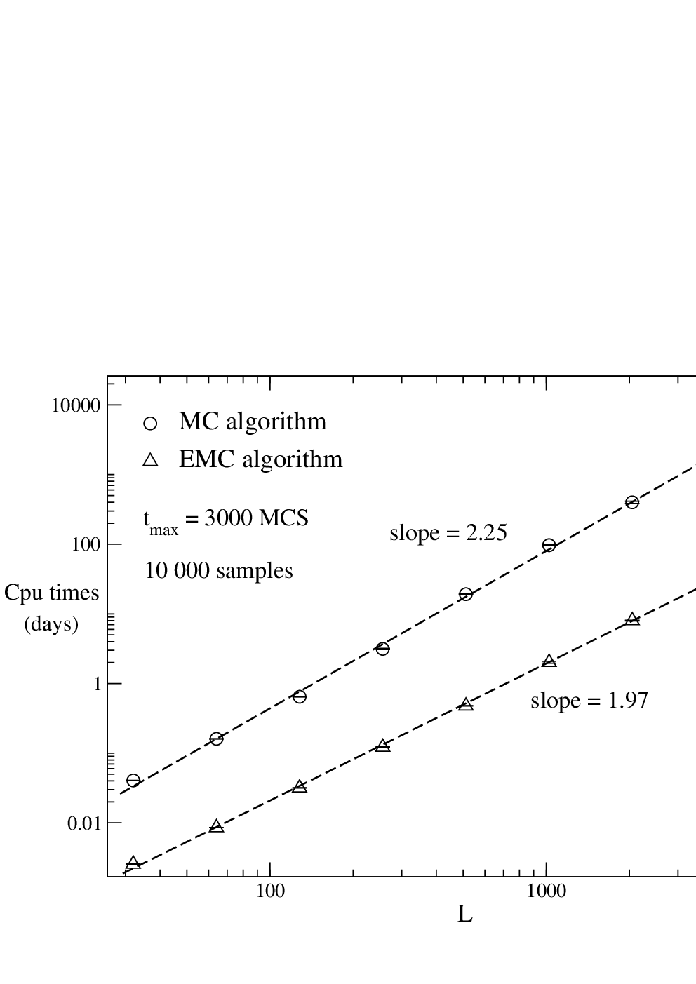
In Fig. 2, the CPU time are shown for these two algorithms. For convenience of the comparison, we set the maximum value of the simulation time $t_{max}=3\penalty\ 000$ MCS and the size of the statistical samples $N_{s}=10\penalty\ 000$. The open circles and open triangles correspond to the CPU time of the Monte Carlo (MC) and MEC algorithms, respectively, with one day as the unit. Generally speaking, the CPU time of the former is nearly $100$ times larger than that of the latter, showing the great superiority of the EMC algorithm. As the lattice size $L$ increases, a power-law behavior is observed for the CPU time, and the slope $1.97$ of the EMC algorithm is a bit smaller than $2.25$ of the usual Monte Carlo algorithm which means that the EMC algorithm is more efficient when the system size becomes larger, pointing to a possibility of the large-scale simulations for the depinning transition in DRFIM. Since the CPU time obeys $\delta t\sim L^{2}$, a linear time complexity, i.e., $O(n)$, is revealed for the EMC algorithm, further confirming that the algorithm is optimized.

Besides, the accuracy of EMC algorithm are also be carefully examined, in comparison with that of the usual Monte Carlo algorithm. As shown in Fig. 3, the velocity of the domain interface $v(t)$, as the order parameter of the depiinning transition, is displayed as a function of the time $t$ for different lattice sizes $L$. The symbols represent numerical results obtained by the usual Monte Carlo method, and solid and dash-dotted lines correspond to those obtained by the EMC algorithm. A driving field $H=1.2933$ is then used, which was reported as the transition point at the disorder strength $\Delta=1.5$ [48, 50]. With the scaling form in Eq. (10), the dynamic behavior $v(t)\sim t^{-\beta/\nu z}f(t/L^{z})$ is deduced at $\tau=0$, and the finite-size effect described by $f(t/L^{z})$ can be easily controlled, i.e., it rapidly approaches a constant as $L$ increases.

Two distinguishable scaling regimes are found in numerical results, which are separated by a characteristic time scale $t_{L}\sim L^{z}$. When $t<t_{L}$, the symbols of different lattice size $L$ nicely collapse to a master curve $v(t)\sim t^{-\beta/\nu z}$ with the slope $0.217(2)$, meaning an absence of the finite-size effect. The symbols are overlap with the corresponding solid lines, confirming that the numerical results obtained by these two algorithms are almost the same. Though the deviations of the symbols and lines are observed in the second time regime with $t>t_{L}$, one can use a sufficiently large lattice size, e.g., $L=8192$, to make sure all the results in this paper staying in the first regime with $t_{max}<t_{L}$. Consequently, the EMC algorithm not only significantly saves the computing cost, but also has a high accuracy. Interestingly, the tail of the master curve, depicted by the dash-dotted line, exhibits a significant deviation from the power-law behavior marked by the dashed line, as shown in Fig. 3. It indicates that the driving field $H=1.2933$ is smaller than the exact transition point $H_{c}$.

Extensive numerical simulations are performed with the EMC algorithm to identify the depinning transition in disordered media. Unless otherwise stated, the lattice size $L=8192$ is used in the following. Fig. 4 shows the dynamic relaxation of the number $N(t)$ of the activated spin under different driving fields $H$. Similar with the velocity $v(t)$ of the domain interface, the number $N(t)$ drops rapidly down for a small $H$, while approaches a constant for a large $H$. Searching for the best power-law behavior, one can locate the transition field $H_{c}=1.29371(4)$, much more precise than the previous one $1.2933(2)$ obtained with the usual Monte Carlo method [48, 50]. In addition, another simulations with the lattice size $L^{\prime}=12\penalty\ 000$ are also carried out. Rescaled by a factor $L^{\prime}/L$, the solid line, i.e., $N(t)$ at $L=8192$, is in perfect agreement with the open circles and stars, corresponding to $N(t)$ and $v(t)L^{\prime}$ at $L^{\prime}=12\penalty\ 000$, respectively, confirming that finite-size effect is already negligibly small. Moreover, an almost-perfect power-law decay $N(t)=v(t)L\sim t^{\beta/\nu z}$ is observed at the transition point $H_{c}=1.29371$. A direct measurement from the slope of the fitting yields $\beta/\nu z=0.203(1)$.

To obtain a more accurate value of the transition point, the error of the power-law fitting $\chi^{2}/{\rm DoF}$ [55] is carefully examined within a very narrow $H$-regime $[1.29366,1.29375]$, as shown in the inset of Fig. 4. The critical point can be determined by judging the location of the minimization of $\chi^{2}/{\rm DoF}$. For different waiting time $t_{0}=50,100$ and $200$ MCS, an almost same value $H_{c}=1.29371(1)$ is obtained, further showing that our result is robust and precise. In Fig. 5, the logarithmic derivatives of $N(t)$ and $v(t)$ in the neighborhood of $H_{c}=1.29371$ are shown with open circles and stars, respectively. With the scaling form in Eq. (13), the exponent $1/\nu z=0.677(3)$ is measured from the slope of the dashed line. To extend the fitting to earlier times of the numerical data, the correction to scaling is considered with the form in Eq. (17). The exponent $1/\nu z=0.68(1)$ is then determined, consistent with the previous one within the error bar.

Besides the velocity of the domain interface, we also investigate the roughness function $\omega^{2}(t)$ and the correlation function $C(r,t)$ defined in Eqs. (6) and (7), respectively. With the scaling form of $C(r,t)$ in Eq. (14), numerical data at different time $t$ collapse to the curve at $t^{\prime}=10\penalty\ 240$ MCS by rescaling $r$ to $[\xi(t^{\prime})/\xi(t)]r$ and C(r,t) to $[\omega^{2}(t^{\prime})/\omega^{2}(t)]C(r,t)$. Adopting this data-collapse technique [56], one can extract the nonequilibrium correlation length $\xi(t)$ from the correlation function $C(r,t)$. The results are shown in Fig. 6 at the depinning field $H_{c}=1.29371$ for the domain interface with $\Delta=1.5$ (open circles) and the bulk with $\Delta=0$ (open triangles). Power-law behaviors are observed for both of them with the slopes $1/z=0.837(5)$ and $1/z_{b}=0.663(5)$, respectively. However, an obvious deviation from the power law is found in the early times of the curve composed of open circles, thereby correction to scaling should be considered. With the correction form in Eq. (17), we refine the value of the exponent $1/z=0.896(7)$. Moreover, a perfect coincidence between the open circles and pluses are observed, pointing to the relationship $F(t)\sim\xi(t)$, consistent with the prediction in earlier work [48]. In the inset, the scaling function $\widetilde{C}(r/\xi(t))$ is plotted as the function of $r$. Data of different time $t$ nicely collapse to the curve at $t=10\penalty\ 240$ MCS by rescaling $r$ to $r/\xi(t)$, confirming the accurate of the correlation length. Moreover, the exponent $2\zeta_{loc}=1.53(4)$ is measured by the fitting with Eq. (16).

With the correlation length $\xi(t)$ at hand, we then study the roughening process of the domain interface at the depinning transition. In Fig. 6, $\omega^{2}(t)$ is plotted as a function of $\xi(t)$ on a log-log scale. Obviously, $\omega^{2}(t)$ at the transition field $H_{c}=1.29371$ with $\Delta=1.5$ shows a cleaner power-law behavior than $\xi(t)$ does, and the roughness exponent $2\zeta=2.00(2)$ is measured based on Eq. (15). It is much larger than $2\zeta_{b}=0.97(1)$ for the bulk with $\Delta=0$. In the inset, the roughness function $\omega(t)$ is displayed with the solid line, and the direct measurement of the slope yields $2\zeta/z=1.65(2)$.

Finally, we summarize all the measurements of the critical exponents in Table. 1. The transition field $H_{c}=1.29371(1)$ is more precise than the earlier result $1.2933(2)$ [48, 50], and significant deviations (reaching nearly $10\%\sim 30\%$) are also observed in the exponents $\nu,z$, and $\zeta$, showing the necessity of large-scale simulations for the depinining. For comparison, the exponents of the QEW equation [28, 34] are also shown in the table with the same lattice size $L=8\penalty\ 192$. The contention that the depinnning transition of the DRFIM and QEW equation are not in a same universality class is supported by the distinct differences of the exponents between these two models, especially in $\beta,z$, and $\zeta$. According to the arguments in Refs.[48, 49], the difference is mainly due to the overhangs and islands created in the depinning process of DRFIM.

Does the depinning transition in the DRFIM belong to a universality class? To solve this issue, comprehensive simulations have been performed for different strengthes of the disorder (varying from $\Delta=0$ to $10$) in DRFIM and different types of the disorder, taking the random-bond disorder in the DBDIM as another example. As shown in Fig. 8, the phase boundary is displayed separating the depinning phase from the pinning phase. The vertical dash-dotted line indicates a critical value $\Delta_{c}=1.0$ of the disorder, where the phase transition is of first order when $\Delta\leq\Delta_{c}$ and of second order when $\Delta>\Delta_{c}$. In both of them, linear behaviors are observed with the slopes $1.00$ and $0.213(4)$, respectively. Unfortunately, the disorder strength $\Delta=1.5$ which has been carefully investigated before is nearby the crossover between these two regimes, suggesting that the values of the exponents in Table. 1 may be $\Delta$-dependent.

As an example, the velocity of the domain interface $v(t)$ at the critical point $\Delta_{c}=1.0$ is shown in Fig. 9. Quite different from those in Figs. 3 and 4, $v(t)$ decays exponentially at $H\leq 0.99999$, and approaches a nonzero constant at $H\geq 1.00000$. A huge jump is then found in the steady-state velocity as the driving field is changed by only a paltry amount of $10^{-5}$, inferring that it is a typical first-order phase transition, and the transition point is $H_{c}=1.00000$. Similar phenomena are also found for the disorder strength $\Delta<\Delta_{c}$. While power-law decays of the domain interface are found at $H_{c}$ for $\Delta>\Delta_{c}$, corresponding to the second-ordered phase transition. The critical exponents with respect to the disorder strength $\Delta$ are investigated carefully, and a scaling relation $\beta/\nu z+\zeta/z=0.99(1)$ is revealed in Fig. 10 for sufficiently strong disorder, consistent with the prediction of the scaling theory $\beta=\nu(\zeta-z)$ in the QEW equation [36, 37]. It means that the roughness exponent $\zeta$ is not independent, and the roughening process of the domain interface $\omega^{2}(t)\sim t^{2\zeta/z}$ is merely induced by the depinning transition with $h(t)\sim t^{1-\beta/\nu z}$. In contrast, the other scaling relation $\nu=1/(2-\zeta)$ is apparently violated, indicating the breaking down of the statistical tilt symmetry.

In addition, the robustness of the exponents $\zeta/z$ and $1-\beta/\nu z$ is affirmed in Fig. 10 for a wide window $\Delta\in[0,10]$, indicating a universality class. Furthermore, we summary the values of the exponents $\beta,\nu,z,\zeta,\zeta_{loc}$, and $\beta/\nu z+\zeta/z$ in Table. 2 for two cases with the disorder strengthes $\Delta=5.0$ and $10.0$, respectively. For each exponent, a perfect consistency between these two cases is found within the error bars. In the same way, the depinning transition in the DBDIM is also investigated with a Gaussian distribution of the random-bond disorder. The standard deviation $\sigma=1.5$ is used in the simulations, which is already sufficiently large for the depinning transition. The results of these critical exponents listed in Table. 2 are almost the same with those obtained from the DRFIM with $\Delta=5.0$ and $10.0$, but significantly differ from those of the QEW equation shown in Table. 1. It further supports our conclusion that the depinning transition in the Ising-type lattice models belong to a new universality class, though the scaling relation $\beta=\nu(z-\zeta)$ is still valid.

References

- [1] S. Lemerle, J. Ferré, C. Chappert, V. Mathet, T. Giamarchi, P. L. Doussal, Domain wall creep in an ising ultrathin magnetic film, Phys. Rev. Lett. 80 (1998) 849. doi:10.1103/PhysRevLett.80.849.
- [2] C. J. Bolech, A. Rosso, Universal statistics of the critical depinning force of elastic systems in random media, Phys. Rev. Lett. 93 (2004) 125701. doi:10.1103/PhysRevLett.93.125701.
- [3] P. L. Doussal, K. J. Wiese, E. Raphael, R. Golestanian, Can nonlinear elasticity explain contact-line roughness at depinning?, Phys. Rev. Lett. 96 (2006) 015702. doi:10.1103/PhysRevLett.96.015702.
- [4] A. B. Kolton, A. Rosso, T. Giamarchi, W. Krauth, Dynamics below the depinning threshold in disordered elastic systems, Phys. Rev. Lett. 97 (2006) 057001. doi:10.1103/PhysRevLett.97.057001.
- [5] M. B. Luo, X. Hu, Depinning and creep motion in glass states of flux lines, Phys. Rev. Lett. 98 (2007) 267002. doi:10.1103/PhysRevLett.98.267002.
- [6] B. Bakó, D. Weygand, M. Samaras, W. Hoffelner, M. Zaiser, Dislocation depinning transition in a dispersion-strengthened steel, Phys. Rev. B 78 (2008) 144104. doi:10.1103/PhysRevB.78.144104.
- [7] M. Y. Im, L. Bocklage, P. Fischer, G. Meier, Direct observation of stochastic domain-wall depinning in magnetic nanowires, Phys. Rev. Lett. 102 (2009) 147204. doi:10.1103/PhysRevLett.102.147204.
- [8] J. Gorchon, S. Bustingorry, J. Ferré, V. Jeudy, A. B. Kolton, T. Giamarchi, Pinning-dependent field-driven domain wall dynamics and thermal scaling in an ultrathin Pt/Co/Pt magnetic film, Phys. Rev. Lett. 113 (2014) 027205. doi:10.1103/PhysRevLett.113.027205.
- [9] M. Rost, L. Laurson, M. Dubé, M. Alava, Fluctuations in fluid invasion into disordered media, Phys. Rev. Lett. 98 (2007) 054502. doi:10.1103/PhysRevLett.98.054502.
- [10] L. Du, H. Bodiguel, A. Colin, Thermally activated depinning motion of contact lines in pseudopartial wetting, Phys. Rev. E 90 (2014) 012402. doi:10.1103/PhysRevE.90.012402.
- [11] G. Blatter, M. V. Feigel’man, V. B. Geshkenbein, A. I. Larkin, V. M. Vinokur, Vortices in high-temperature superconductors, Rev. Mod. Phys. 66 (1994) 1125. doi:10.1103/RevModPhys.66.1125.
- [12] S. Okuma1, A. Motohashi, Critical behavior associated with transient dynamics near the depinning transition, New J. Phys. 14 (2012) 123021. doi:10.1088/1367-2630/14/12/123021.
- [13] S. Brazovskii, T. Nattermann, Pinning and sliding of driven elastic systems: from domain walls to charge density waves, Adv. Phys. 53 (2004) 177. doi:10.1080/00018730410001684197.
- [14] M. LeBlanc, L. Angheluta, K. Dahmen, N. Goldenfeld, Universal fluctuations and extreme statistics of avalanches near the depinning transition, Phys. Rev. E 87 (2013) 022126. doi:10.1103/PhysRevE.87.022126.
- [15] S. Atis, A. K. Dubey, D. Salin, L. Talon, P. L. Doussal, K. J. Wiese, Experimental evidence for three universality classes for reaction fronts in disordered flows, Phys. Rev. Lett. 114 (2015) 234502. doi:10.1103/PhysRevLett.114.234502.
- [16] M. Ovaska, L. Laurson, M. J. Alava, Quenched pinning and collective dislocation dynamics, Sci. Rep. 5 (2015) 10580. doi:10.1038/srep10580.
- [17] J. C. Lee, K. J. Kim, J. Ryu, K. W. Moon, S. J. Yun, G. H. Gim, K. S. Lee, K. H. Shin, H. W. Lee, S. B. Choe, Universality classes of magnetic domain wall motion, Phys. Rev. Lett. 107 (2011) 067201. doi:10.1103/PhysRevLett.107.067201.
- [18] D. Bang, H. Awano, Domain wall motion in Tb/Co multilayer wires with a large domain wall depinning field, J. Appl. Phys. 115 (2014) 17D512. doi:10.1063/1.4868918.
- [19] Y. J. Shin, B. C. Jeon, S. M. Yang, I. Hwang, M. R. Cho, D. Sando, S. R. Lee, J. G. Yoon, T. W. Noh, Suppression of creep-regime dynamics in epitaxial ferroelectric bifeo3 films, Sci. Rep. 5 (2015) 10485. doi:10.1038/srep10485.
- [20] A. J. Ramsay, P. E. Roy, J. A. Haigh, R. M. Otxoa, A. C. Irvine, T. Janda, R. P. Campion, B. L. Gallagher, J. Wunderlich, Optical spin-transfer-torque-driven domain-wall motion in a ferromagnetic semiconductor, Phys. Rev. Lett. 114 (2015) 067202. doi:10.1103/PhysRevLett.114.067202.
- [21] C. Wuth, L. Kolbe, G. Meier, Thermally activated stochastic domain-wall depinning in ferromagnetic nanowires, J. Appl. Phys. 114 (2013) 103901. doi:10.1063/1.4819808.
- [22] V. O. Dolocan, Domain wall pinning and interaction in rough cylindrical nanowires, Appl. Phys. Lett. 105 (2014) 162401. doi:10.1063/1.4899128.
- [23] S. Fukami, J. Ieda, H. Ohno, Thermal stability of a magnetic domain wall in nanowires, Phys. Rev. B 91 (2015) 235401. doi:10.1103/PhysRevB.91.235401.
- [24] P. M. Shepley, A. W. Rushforth, M. Wang, G. Burnell, T. A. Moore, Modification of perpendicular magnetic anisotropy and domain wall velocity in Pt/Co/Pt by voltage-induced strain, Sci. Rep. 5 (2015) 7921. doi:10.1038/srep07921.
- [25] M. Yamanouchi, J. Ieda, F. Matsukura, S. E. Barnes, S. Maekawa, H. Ohno, Universality classes for domain wall motion in the ferromagnetic semiconductor (ga,mn)as, Science 317 (2007) 1726. doi:10.1126/science.1145516.
- [26] M. Hayashi, L. Thomas, R. Moriya, C. Rettner, S. S. P. Parkin, Current-controlled magnetic domain-wall nanowire shift register, Science 320 (2008) 209. doi:10.1126/science.1154587.
- [27] S. S. P. Parkin, M. Hayashi, L. Thomas, Magnetic domain-wall racetrack memory, Science 320 (2008) 190. doi:10.1126/science.1145799.
- [28] E. E. Ferrero, S. Bustingorry, A. B. Kolton, Nonsteady relaxation and critical exponents at the depinning transition, Phys. Rev. E 87 (2013) 032122. doi:10.1103/PhysRevE.87.032122.
- [29] H. H. Boltz, J. Kierfeld, Depinning of stiff directed lines in random media, Phys. Rev. E 90 (2014) 012101. doi:10.1103/PhysRevE.90.012101.
- [30] E. A. Jagla, Creep dynamics of viscoelastic interfaces, Europhys. Lett. 105 (2014) 46003. doi:10.1209/0295-5075/105/46003.
- [31] Y. J. Chen, S. Zapperi, J. P. Sethna, Crossover behavior in interface depinning, Phys. Rev. E 92 (2015) 022146. doi:10.1103/PhysRevE.92.022146.
- [32] J. M. López, M. A. Rodríguez, Interface dynamics at the depinning transition, J. Phys. I France 7 (1997) 1191. doi:10.1051/jp1:1997116.
- [33] A. B. Kolton, A. Rosso, E. V. Albano, T. Giamarchi, Short-time relaxation of a driven elastic string in a random medium, Phys. Rev. B 74 (2006) 140201(R). doi:10.1103/PhysRevB.74.140201.
- [34] J. M. Kim, H. Choi, Depinning transition of the quenched edwards-wilkinson equation, J. Korean Phys. Soc. 48 (2006) S241.
- [35] O. Duemmer, W. Krauth, Critical exponents of the driven elastic string in a disordered medium, Phys. Rev. E 71 (2005) 061601. doi:10.1103/PhysRevE.71.061601.
- [36] T. Nattermann, S. Stepanow, L. Tang, H. Leschhorn, Dynamics of interface depinning in a disordered medium, J. Phys. II France 2 (1992) 1483. doi:10.1051/jp2:1992214.
- [37] P. L. Doussal, K. J. Wiese, P. Chauve, Two-loop functional renormalization group theory of the depinning transition, Phys. Rev. B 66 (2002) 174201. doi:10.1103/PhysRevB.66.174201.
- [38] M. Jost, J. Heimel, T. Kleinefeld, Domain-wall roughening in alloy films, Phys. Rev. B 57 (1998) 5316. doi:10.1103/PhysRevB.57.5316.
- [39] P. J. Metaxas, J. P. Jamet, A. Mougin, M. Cormier, J. Ferré, V. Baltz, B. Rodmacq, B. Dieny, R. L. Stamps, Creep and flow regimes of magnetic domain-wall motion in ultrathin pt/co/pt films with perpendicular anisotropy, Phys. Rev. Lett. 99 (2007) 217208. doi:10.1103/PhysRevLett.99.217208.
- [40] M. Eltschka, M. Wötzel, J. Rhensius, S. Krzyk, U. Nowak, M. Kläui, T. Kasama, R. E. D. Borkowski, L. J. Heyderman, H. J. van Driel, R. A. Duine, Nonadiabatic spin torque investigated using thermally activated magnetic domainwall dynamics, Phys. Rev. Lett. 105 (2010) 056601. doi:10.1103/PhysRevLett.105.056601.
- [41] A. Goussev, J. M. Robbins, V. Slastikov, Domain-wall motion in ferromagnetic nanowires driven by arbitrary time-dependent fields: An exact result, Phys. Rev. Lett. 104 (2010) 147202. doi:10.1103/PhysRevLett.104.147202.
- [42] T. Gerhardt, A. Drews1, G. Meier, Current-driven domain wall depinning from an anisotropy boundary in nanowires, J. Phys.: Condens. Matter 26 (2014) 206001. doi:10.1088/0953-8984/26/20/206001.
- [43] U. Nowak, K. D. Usadel, Influence of temperature on the depinning transition of driven interfaces, Europhys. Lett. 44 (1998) 634. doi:10.1209/epl/i1998-00519-4.
- [44] F. Colaiori, G. Durin, S. Zapperi, Loss separation for dynamic hysteresis in ferromagnetic thin films, Phys. Rev. Lett. 97 (2006) 257203. doi:10.1103/PhysRevLett.97.257203.
- [45] B. Koiller, M. O. Robbins, Growth and morphology transitions in anisotropic disordered media, Phys. Rev. B 82 (2010) 064202. doi:10.1103/PhysRevB.82.064202.
- [46] B. Xi, M.-B. Luo, V. M. Vinokur, X. Hu, Depinning transition of a domain wall in ferromagnetic films, Sci. Rep. 5 (2015) 14062. doi:10.1038/srep14062.
- [47] L. A. N. Amaral, A. L. Barabási, H. A. Makse, H. E. Stanley, Scaling properties of driven interfaces in disordered media, Phys. Rev. E 52 (1995) 4087. doi:10.1103/PhysRevE.52.4087.
- [48] N. J. Zhou, B. Zheng, Y. Y. He, Short-time domain-wall dynamics in the random-field ising model with a driving field, Phys. Rev. B 80 (2009) 134425. doi:10.1103/PhysRevB.80.134425.
- [49] N. J. Zhou, B. Zheng, Dynamic effect of overhangs and islands at the depinning transition in two-dimensional magnets, Phys. Rev. E 82 (2010) 031139. doi:10.1103/PhysRevE.82.031139.
- [50] X. P. Qin, B. Zheng, N. J. Zhou, Universality class of the depinning transition in the two-dimensional ising model with quenched disorder, J. Phys. A: Math. Theor. 45 (2012) 115001. doi:10.1088/1751-8113/45/11/115001.
- [51] L. Roters, A. Hucht, S. Lübeck, U. Nowak, K. D. Usadel, Depinning transition and thermal fluctuations in the random-field ising model, Phys. Rev. E 60 (1999) 5202. doi:10.1103/PhysRevE.60.5202.
- [52] B. Zheng, Monte carlo simulations of short-time critical dynamics, Int. J. Mod. Phys. B 12 (1998) 1419. doi:10.1142/S021797929800288X.
- [53] H. J. Luo, L. Schülke, B. Zheng, Dynamic approach to the fully frustrated xy model, Phys. Rev. Lett. 81 (1998) 180. doi:10.1103/PhysRevLett.81.180.
- [54] L. Roters, S. Lübeck, K. D. Usadel, Creep motion in a random-field ising model, Phys. Rev. E 63 (2001) 026113.
- [55] C. Chatelain, B. Berche, W. Janke, P. E. Berche, Softening of first-order transition in three-dimensions by quenched disorder, Phys. Rev. E 64 (2001) 036120. doi:10.1103/PhysRevE.64.036120.
- [56] N. J. Zhou, B. Zheng, Nonsteady dynamic properties of a domain wall for the creep state under an alternating driving field, Phys. Rev. E 90 (2014) 012104. doi:10.1103/PhysRevE.90.012104.