BCJ Relations for One-Loop QCD Integral Coefficients
Abstract
We present a set of one-loop integral coefficient relations in QCD. The unitarity method is useful for exposing one-loop amplitudes in terms of tree amplitudes. The coefficient relations are induced by tree-level BCJ amplitude relations. We provide examples for box, triangle, and bubble coefficients. These relations reduce the total number of independent coefficients needed to calculate one-loop QCD amplitudes.
I Introduction
Devising efficient methods for calculating scattering amplitudes has been useful to confirm the validity of the Standard Model. Even at tree level, the number of Feynman diagrams dramatically increases as the number of legs increases. For seven, eight, and nine external gluons there are already 2485, 34300, and 559405 Feynman diagrams needed at tree level [1]. Of course, with modern techniques we can obtain the amplitude without calculating any Feynman diagrams. At tree-level, the amplitude is decomposed into a color-stripped partial amplitude , which separates the color from the kinematics. The Parke–Taylor formula gives simple form of maximally helicity violating (MHV) or anti-MHV partial amplitudes [2, 3]. On shell recursion developed by Britto, Cachazo, Feng and Witten (BCFW) can be used to find any helicity [4, 5]. To compute the total amplitude , we need to compute the partial amplitudes , corresponding to the different permutations of the legs. However, not all partial amplitudes are independent. Since we have a trace over the color generators, the partial amplitudes have cyclic symmetry, leaving independent partial amplitudes. The partial amplitudes also satisfy a reflection property and the U(1) photon decoupling identity, which reduces the number of independent partial amplitudes. (See e.g. Refs. [1, 6].) Remarkably, there are more tree level partial amplitude identities. The Kleiss–Kuijf relations [7] reduces the number of independent partial amplitudes to . Furthermore, the Bern–Carrasco–Johansson (BCJ) amplitude relations [8, 9, 10, 11] give independent partial amplitudes. This paper applies these ideas to reduce the number of independent integral coefficients at one loop.
At one-loop, we consider on-shell diagrams instead of Feynman diagrams. We apply the unitary method finding the value of the loop amplitude with the loop momentum on-shell. Furthermore, when we apply the unitarity cuts, one-loop amplitudes with massless external legs can be reconstructed in terms of products of tree amplitudes. The coefficients of basis integrals are fully determined from four-dimensional tree amplitudes [12, 13] and rational remainders from -dimensional ones [14, 15, 16, 17, 18]. For a modern review of on-shell and unitarity methods for one-loop QCD amplitudes, we refer the reader to Ref. [19].
Since tree amplitudes determine the integral coefficient within the unitarity approach, we expect that the integral coefficients satisfy similar identities as the tree amplitudes themselves. In particular, we show that the tree-level BCJ amplitude relations can be used to derive integral coefficient identities. Since the loop momenta always have two on-shell solutions, we have to decompose the integral coefficient into two pieces. It is these pieces which actually satisfy the coefficient relations, rather than the total coefficient.
We demonstrate that tree level identities significantly decrease the total number of independent integral coefficients. These relations could be used to either improve the efficiency of one-loop amplitude calculations or to provide a stability or other cross checks for the integral coefficients (e.g. see Ref. [20]).
This paper is organized as follows: To demonstrate that the one-loop integral coefficients satisfy BCJ integral coefficient relations, we start by reviewing the tree-level BCJ relations and the unitarity method in section II. In section III, we derive the general expressions for the one-loop BCJ integral coefficient relations from the tree-level BCJ amplitude relations. In section IV, we explicitly provide examples and confirm that the BCJ integral coefficient relation is satisfied. Finally, we conclude and briefly discuss possible future work in section V.
II From Trees to Loops
II.1 Introduction to Tree-Level BCJ Amplitude Relations
In this section, we review the unitarity method and the necessary tree-level identities needed. In the next section, we will show that the BCJ amplitude relations can be used with the unitarity method to find new relations between integral coefficients. Therefore, we start by reviewing the BCJ amplitude relations for future reference.
We focus on color-stripped partial amplitude. The color-stripped partial amplitude, , is related to the full amplitude via [6]
| (1) |
where represents the permutations of external legs divided by the cyclic permutations which are removed because they would give the same color trace. Partial amplitudes only depend on kinematic variables, and the labels of the partial amplitude signify the momenta and helicities of the particles.
The BCJ amplitude relations at tree level are connected to color-kinematics duality [8]. The duality forces the Jacobi identity on the kinematic numerators, which naturally provide tree-level partial amplitude relations beyond what is contained in the Kleiss–Kuijf relations. The BCJ relations imply that only of the partial amplitudes are independent. A convenient choice is to fix the first 3 legs. At four and five points, the BCJ tree amplitude relations are
| (2) |
The original BCJ paper also includes general -point formulas for generating the BCJ relations. Notice how the BCJ amplitude relations fixes the first three legs for the set of independent partial amplitudes.
To express amplitudes, we will use the spinor-helicity formalism, which gives remarkably compact expressions for certain tree amplitudes. Tree amplitudes with zero or one plus/minus helicities are zero (except for the three-point amplitudes). The -point Parke–Taylor formula [2, 3] expresses the MHV partial amplitudes in a remarkably simple manner,
| (3) |
To find all other helicity configurations, BCFW recursion, for example, can be applied to calculate any amplitude from the Parke–Taylor formula [4]. (See, for example, Ref. [21] for an exhaustive review with examples.)
II.2 Unitary Cuts and One-Loop Integral Basis Coefficients
We now review the unitarity method, which is used find one-loop amplitudes as a linear combination of integral coefficients times basis integrals. At one loop any massless amplitude can be decomposed into a set of basis integrals consisting of scalar boxes, triangles, and bubbles, plus rational terms for QCD [22, 23, 24]. This reduces the problem of calculating one-loop amplitudes to determining a set rational coefficients.
Britto, Cachazo, and Feng showed how generalized unitarity could be used to find the box coefficients [25]. The work of Ossola, Papadopolous, and Pittau [26] and Forde [27] extends this to the triangle and bubble coefficients. Unitarity cuts can be used to recycle tree amplitudes into the loop level integral coefficients. Therefore, we can generate all one-loop amplitudes from tree amplitudes; the coefficients are simply products of tree amplitudes with loop momenta on-shell.
We will study the boxes, triangles, and bubbles necessary for massless QCD in the following subsections. In particular, we are interested in the total number of cuts needed as well as the loop momentum solutions for such cuts. In order to apply unitarity cuts to a diagram, we put the loop momenta on shell which is imposed on all internal lines in Fig. 1.
To calculate the full one-loop amplitude, each possible unitary cut must be evaluated. Using generalized unitarity this allows us to determine the coefficients of basis integrals in terms of which the amplitude is expressed,
| (4) |
where runs over the total number of basis integrals , Inti is a scalar integral, and represents the rational terms which will be neglected throughout this work.

II.2.1 Box Cuts

To start our study of QCD amplitudes, we focus on the box coefficients which can be determined from the box cuts shown in Fig. 1. Next, we classify the different types of box cuts. There are zero-mass, one-mass, two-mass-e, two-mass-h, three-mass, and four-mass box cuts, which is shown in Fig. 2. Only the four-point amplitudes have a zero-mass box. There are -point one-mass boxes for , since there are ways that the particles could be put together in the corner. For two-mass-h boxes, there are ways with . The number of two-mass-e boxes would be the same, but we are now overcounting by a factor of two due to the symmetry of the two single legs being across from each other. Therefore, there are two-mass-h boxes with . When , there are three-mass boxes. For four-mass boxes, there are three contributing boxes. If and , then there are contributing boxes. This corresponds to when all four corners of the box cut have the same number of legs, such as the only four-mass eight-point cut would have. If and is even, then there are an additional . Finally, if , then there are additional four-mass boxes.
The unitarity cuts put the loop momenta on-shell, which gives a quadratic equation with two solutions. If there is at least one massless leg on the cut, we utilize the following compact solution [20, 28],
| (5) |
Note that the ‘’ solution is simply the complex conjugate of the ‘’ solution. If we have a four-mass box, then we must resort to using the more lengthy solution provided by Britto, Cachazo, and Feng [25]. (See Ref. [29] for loop momentum solutions in .)
To obtain an arbitrary box coefficient, we simply apply a unitarity cut and multiply the four corresponding tree amplitudes together:
| (6) |
where the on the coefficients refers to the two loop solutions, are the tree amplitudes from the cuts, and is the total number of boxes. Note that the true integral coefficient is the sum of the two coefficients , but we must keep these separate to find the coefficient relations.
II.2.2 Triangles
Next consider the triangle integral coefficients. We start with the triangles by counting the number of triangle cuts. There are the one-mass, two-mass, and three-mass triangle cuts, which are shown in Fig. 3. Once again, there are one-mass cuts. Similar to the two-mass-e box cut, there are two-mass triangle cuts. Finally, for the three-mass, we have an equation similar to the four-mass box cut, but no choose function is needed since it would have been choose 1. If and , then we have contributing cuts. Furthermore, if , then we have an additional .

For finding the loop solutions for triangle diagrams, a parameter is introduced to represent the undetermined degree of freedom from having only three unitarity cuts. After converting Forde’s loop solution [27] into our notation, we find
| (7) |
where , , and . The four-momentum representation of the loop momentum solution is
| (8) |
We can in principle consider four triangle loop solutions, since there are two loop momenta and two gammas. However, if or , then there is only one non-zero solution for gamma. In either case, we simply average over the two or four solutions, including the two loop momenta. To find the second loop solution, we can take the complex conjugate, or simply switch all of the angle brackets with the square brackets.
Note that our ’s are a bit different than Forde, since we use different conventions for the loop and external momenta. Just as Forde showed, we find that , for . Our conventions match those of Refs. [20, 29].
Following Forde’s procedure to find the -independent triangle coefficient we take
| (9) |
where is two or four, depending on if there are one or two independent values for gamma. The symbol instructs one to Taylor expand with respect to around infinity and keep the term to obtain the triangle integral coefficients.
II.2.3 Bubbles

Next, we review the extraction of the bubble coefficient. Counting the number of bubble cuts is much simpler, since there are only one-mass and two-mass diagrams. There are one-mass cuts and two-mass cuts, shown in Fig. 4. The bubble loop momentum solution has two arbitrary parameters, and . Instead of using , any arbitrary massless vector can be used. It is often convenient to choose it to be the last leg on , which gives a simple and . We define in terms of the massless spinor.
| (10) |
Now, we are ready to express the loop solution in terms of and .
| (11) |
From these we can find loop momenta,
| (12) |
To find a bubble coefficient, we first find the bubble cut contribution to the bubble coefficient, leaving in the and dependence,
| (13) |
To obtain the full bubble coefficient independent of or , one can use the methods described in Refs. [26, 27, 18, 29, 20]. The expression for the bubble cut contribution to coefficient is
| (14) |
The bubble coefficient includes contributions from the triangles, but we will show that these contributions also satisfy the BCJ integral coefficient relations when we review the triangles. We will not review the bubble extraction in full detail, since we show that the triangle coefficient satisfies the new coefficient relations for all orders of , implying that it hold for the total bubble coefficient as well.
Our goal is to understand how tree-level amplitude relations can be used to create loop-level integral coefficient relations. The BCJ amplitude relations are needed, since the ordering of the two loop momenta for any tree amplitude is already fixed. Since the relations fix the third leg, we can fix one of the external legs for any of the isolated tree amplitudes. We see that one-loop integral coefficient relations naturally arise from the tree-level BCJ relations.
III One-Loop Amplitude Coefficient Relations
Now that we reviewed the calculation of integral coefficients in arbitrary one-loop amplitudes, we focus on relations between these coefficients. To start, we count the number of integral coefficients needed before the BCJ integral coefficient relations are introduced.
Since the coefficient relations we will derive are independent of the external helicities, we will typically focus on MHV amplitudes for simplicity. Fixing the external helicity configuration, there are external leg orderings, but the properties of the color trace leave only to consider. The factor comes from the cyclic symmetry and the factor of comes from the reflective symmetry of the trace over the color generators. Therefore, one would naively expect there to be independent integral coefficients, where is the number of cuts made per ordering of external momenta. In this section, we will show that the number of independent integral coefficients and tree amplitudes is actually smaller, since the BCJ relations can be recycled into the one-loop level by the unitarity method.
Since each contains two adjacent loop momenta, the BCJ amplitude relations may be easily used if we fix the loop momenta to be the first two legs of the tree amplitude. Let us start by systematically considering possible box cuts of increasing complexity.
III.1 BCJ box integral coefficient identities
We start by considering the simplest box cuts. The first non-trivial example is a five-point one-loop amplitude, which contains only one-mass box cuts. After taking into account the cyclic and reflective symmetries of the partial amplitudes, one would expect independent partial amplitudes. Furthermore, for each of these twelve amplitudes, there are five box cuts, giving 60 coefficients to compute. We would like to demonstrate that after taking the BCJ relations into account, we can reduce the number of independent coefficients to 30.
Consider the following two integral coefficients and , shown in Fig. 5. Not only do they have the same loop solution, but they share three tree amplitudes. Note that the total box coefficient is found by summing the two loop solutions, but we keep these two solutions separate to expose the tree level BCJ amplitude relations. Let us take a closer inspection at the dissimilar tree amplitudes containing
| (15) |

Since the two amplitudes have the same loop momentum solution, we can use the four-point BCJ relation, Eq. (2), to relate the box coefficient. That is,
| (16) |
We look to find all possible five-point box integral coefficient relations. After considering reflection symmetry as well as this new ”twist symmetry” for the legs located on the tree, we find that there are 30 independent five-point coefficients instead of 60. Finding the form of the 30 integral coefficient relations at five-points is as trivial as finding the correct four-point tree-level BCJ amplitude identity, so we will not review the one-mass boxes any further.
Next, consider six-point amplitudes. There are one-mass boxes and two-mass diagrams to consider. We start with the one-mass diagrams. In most cases, there will be multiple one-mass diagrams which have the same loop solution. Consider the following six coefficients: , , , , , and . It is clear that we can use the BCJ relations to remove the calculation of four coefficients. Using Eq. (2),
| (17) |
We see that at six-points, there are even more integral coefficient relations, since there are more cuts with the third leg of the tree amplitude fixed. For counting the number of independent box coefficients needed, it is important to note that not all of the six-point one-mass boxes have six coefficients with the same loop solution. In some cases, there will only be three independent coefficients with the same solution.
Note that at six-points there are 360 one-mass coefficients, yet there are many fewer unique loop solutions. The BCJ relations relate a majority of the coefficients with the same loop momenta. We can see that if there are more than two six-point one-mass box coefficients with the same loop solution up to an overall minus sign to account for reflections, then those extra are dependent on two coefficients. In some cases, you may need to calculate a coefficient which is not needed, but this inconvenience decreases the number of coefficients calculated in the long run. For example, one loop solution has the following three coefficients: , , and . Notice how we can use and as independent basis coefficients, even though we do not need to calculate the second coefficient. It is beneficial, since we are still only calculating two instead of three.
Next, we consider the six-point two-mass-e coefficients. These are a bit more complicated, since there are potentially two tree amplitudes and which can be different for the same loop solution. Once again, we group all of the coefficients with the same loop coefficient. At most, we could have four coefficients which have the same loop solution. For example, consider the following coefficients: , , , and . It is clear that we can relate the second and third coefficient to the first, but the fourth has two twisted corners on and . Expanding the fourth coefficient in terms of tree amplitudes makes the identity more apparent:
| (18) |
From expanding the coefficient in terms of tree amplitudes, we see that two four-point BCJ relations can be used to find this coefficient in terms of . The three relations between the four coefficients mentioned above are
| (19) |
Therefore, we have demonstrated that even if multiple corners of a cut have different orderings, the BCJ relations can still be used multiple times, as long as the related coefficients have the same loop solution.
When continuing this analysis to higher-point amplitudes, we find that the simplification gets better as we increase . The simplification occurs because there are more possible diagrams with the same loop solution. At seven-point, there are 12600 needed box coefficients, but only 1785 independent coefficients. For example, there are 24 permutations of for the coefficient , yet there are only six independent coefficients needed. We will not write out these 18 relations, but it is clear that the BCJ amplitude relations could be used to reduce the number of coefficients. Also, at seven-point we introduce three-mass box coefficients, which could have up to eigth coefficients with the same loop solution. For example, consider twisting , , and on the coefficient . These eight coefficients can all be related to one coefficient, which gives seven relations. Once again, we will not write them down, but it would be easy to generate with the BCJ relations. One would have to be a bit more careful with writing down the relations for the twelve coefficients corresponding to the loop solution contained in . The term gives a dependence on two coefficients, while the would add an overall factor of inverse propagators from Eq. (2).
Interesting eight-point amplitudes to consider would be the four-mass and , since that coefficient would depend on four coefficients. We will not go into deriving the identities, because it is fairly straightforward. Nothing new arises for higher-point boxes besides applying more complicated BCJ relations.
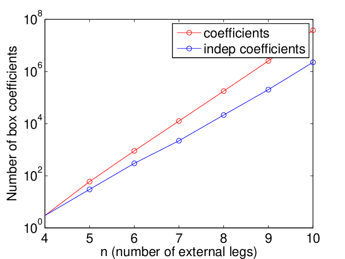
In Fig. 6, we plot the number of box coefficients needed before and after the BCJ integral coefficient relations have been taken into consideration. The log plot shows that as the number of external legs increases, the relations reduce a higher percentage of the coefficients. We see that by eight-points, the number of independent coefficients needed to calculate is roughly an order of magnitude less than what was naively expected.
Finally, we would like to present a formula to count the total number of independent coefficients, after applying the BCJ relations. The boxes are a bit complicated, as there are different countings for the one-mass, two-mass-e, two-mass-h, three-mass, and four-mass boxes. We found the following expression which gave the total number of independent coefficients for .
| (20) |
where is the floor function and sym is a symmetry factor which depends on whether , , , and , are the same or not. Note that , , , and represent the number of external legs on each corner of the box. Naively, we would expect that there would be for each cut topology, but we know that the BCJ relations allow for this new type of twist symmetry, which, up to symmetry factors, divides the number of diagrams by the number of legs on all corners. To get the counting exactly right, we introduced a symmetry factor sym,
| (21) |
The symmetry factor is chosen to properly count the number of needed diagram as well as reflection symmetry. For example, consider a five-point box cut. There is only one type of diagram possible with one corner having two legs and three corners with one leg. There is only one diagram for this specification, yet there is a reflection symmetry, making . For other cases, there could be more diagrams needed, each with their own symmetry properties.
As we have shown, it is no surprise that the box coefficients should satisfy BCJ integral coefficient relations. Next, we investigate how similar identities can be found for the less trivial triangle coefficients.
III.2 BCJ triangle integral coefficient identities
Next, we study how the BCJ relations can be used to simplify triangle integral coefficients. Exactly how the BCJ relations will come into play is less clear, since the loop solutions contain the parameter . In particular, the inverse propagators in the BCJ relations contain loop momenta, and therefore we will end up with expressions for dependent triangle coefficients in terms of the parameter .
We start by considering two coefficients with the same loop solution, say and . We would like to find a way to relate these coefficients by propagators, such that , but we need to be careful with the dependence of the amplitude and the inverse propagators. The first natural guess would be to keep the dependence in the inverse propagators and the coefficient and apply the proper expansion of around infinity, followed by extracting the term. It turns out that this precisely works, as we confirmed numerically. The coefficient identity is
| (22) |
Finding this -dependent coefficient, taking limit as goes to infinity, and taking the term allows for the triangle coefficient to be found:
| (23) |
This shows that the triangle contributions to the bubbles should also satisfy this BCJ identity.
Now that we understand how to properly deal with the parameter, generating triangle coefficient identities is essentially the same as the box coefficients. We group all of the coefficients with the same loop solution together, find the set of independent coefficients, and write down the analogous BCJ relations needed to find the dependent coefficients.
Now that we have demonstrated that the BCJ relations indeed hold for triangle coefficients with Forde’s analytic approach [27], we would like to investigate how we can use them to speed up numerical calculations.
When considering if the BCJ relations speed up performance, there is a caveat since the triangle coefficient only needs the zeroth order term. However, finding with BCJ requires that we keep all of the coefficients in the expansion of for , since the factors of inverse propagators have dependence and will change the zeroth order dependence of the undetermined triangle coefficient. Fortunately, all of these coefficients would be saved for the evaluation of bubble diagrams. Therefore, the only extra computational cost for determining involves finding the coefficients from expanding with respect to . Furthermore, it appears that all of the factors of inverse propagators in all of the BCJ relations, even for higher than four-points, will never have a term for . Even if we did not extract out the boxes and numerically evaluated the coefficients in a Laurent expansion of , we would only need to calculate the zeroth and first three negative powers of the inverse propagator terms. Thus, we have shown that the only extra computation needed the four coefficients for , since only goes up to powers of for Forde’s method.

In Fig. 7, we plot the number of triangle coefficients needed before and after the BCJ integral coefficient relations are taken into account. We notice that the number of triangle coefficients is reduced even less than the boxes. This is due to the fact that less cuts puts more legs on a particular tree amplitude, which makes the BCJ relations more plentiful. We found that the absolute value of the Stirling number of the first kind gives the correct number of independent -point coefficients. Next, we review the bubble integral coefficient identities.
III.3 BCJ bubble integral coefficient identities
We now look to see if the BCJ relations can be utilized with the bubbles. Typically, to calculate the bubble coefficient, one has to subtract out the triangle contributions to the bubble coefficient. However, since we already showed that the triangles follow the BCJ coefficient relations for all orders of , we only need to show that the identity is valid for the bubble cut component of the bubble integral coefficient.
In particular, we analytically and numerically checked that the solution works for the cut for the amplitude . For example, we would like to see how the coefficient of could be found from using the BCJ relations,
| (24) |
Note that to find the true bubble coefficient, we must properly remove the and dependence, such that
| (25) |
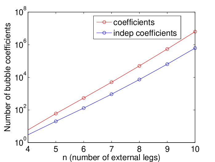
In Fig. 8, we plot the number of bubble coefficients needed before and after the BCJ integral coefficient relations are taken into consideration. As expected, the bubbles are simplified even more heavily than the triangles and boxes. Similar to the triangles, we can use the Stirling number of the first kind to count the number of independent coefficients, but this also includes one-mass coefficients. To find the numbers shown in Fig. 8, we subtracted .
We have clearly demonstrated that the tree-level BCJ amplitude relations can be used to create one-loop integral coefficient relations. However, we note that these BCJ integral coefficient relations are only useful for amplitudes with multiple identical particles, which often is the case for QCD jet processes. However, there will always be other particles interacting with these gluons, which would lessen the number of identities which are suggested by the figures shown throughout this section. These relations could be useful for improving the efficiency of QCD calculations or to check the stability of numerical code.
IV Examples of BCJ integral coefficient relations
IV.1 Box integral coefficient relation example
Let us consider the box integral coefficients and and show explicitly that these coefficients satisfy the integral coefficient relation provided in this work. We start by calculating the diagram explicitly, shown in Fig. 9. In principle, there are eight possible loop helicity configurations, but only one is non-zero for this specific cut. We can write down the coefficient by multiplying by the four tree amplitudes:

| (26) |
where throughout. We can use the loop solution from Eq. (5) and find to be
| (27) |
Right away, it is clear that the positive solution gives zero, since . We continue by only considering the negative loop solution. We can make a choice for and ,
| (28) |
which allows us to simplify the calculation in terms of external spinors.
Futhermore, we can use momentum conservation to express all of the other loop momenta in terms of :
| (29) | |||||
In the last line, we used the Schouten identity to simplify the denominator. Similarly, we can immediately write down the equation for the box coefficient since and have the same helicity, which is given by
| (30) |
Next, we check that the coefficient cut relation holds. To start,
| (31) |
Schouten identities and momentum conservation are used throughout to simplify these expressions. We can see that this is the exact factor which is needed to find from , since
| (32) |
As we have demonstrated, the BCJ integral coefficient identity holds for this five-point box cut example.
IV.2 Triangle integral coefficient relation example
Next, we will show how the BCJ integral coefficient relation holds for a triangle cut. We will choose a four-point cut which has a zero triangle coefficient, but does have non-zero terms for powers of greater than zero. These higher power terms contribute to the bubble coefficient, so we must confirm this in order to show that the BCJ integral coefficient relations work on the total bubble coefficient. In this example, the BCJ relations will be used to find a non-zero triangle integral coefficient from a zero triangle integral coefficient, which is possible since the inverse propagator ratio has t dependence.

We will calculate the triangle cut from the amplitude . There are three nonzero loop helicities which we must consider. We have the three diagrams, which we will label as , , and and are shown in Fig. 10, which when evaluated gives
| (33) |
Choosing and , we find that the following loop solution is
| (34) | |||||
This leaves three non-zero contributions after considering the positive and negative loop solutions,
| (35) |
After expanding about , we find that only the negative solution has non-zero contributions to the triangle and bubble coefficients. Next, we can calculate , which is the same as before picking the term after the expansion about infinity. We find
| (36) |
The fact that there is no zeroth order term shows that there is no triangle coefficient, yet the higher powers of would feed into the bubble coefficient. Let us check the BCJ integral coefficient relation by first calculating the coefficient and then confirming that the two coefficients satisfy the corresponding BCJ relation.
Once again, we can write down expressions for the three amplitudes, which we will refer to as , , and and are shown in Figure 11.

| (37) |
Similarly, there are three non-zero contributions to the triangle/bubble integral coefficient, which are shown below. We used the same loop solution as previously and find
| (38) |
Once again, we find that the positive solution has no contribution to the bubble or triangle coefficient. Interestingly enough, the negative solution does have a non-zero triangle integral coefficient. Since the analytic expression for this amplitude is a bit lengthy, we will only report the zeroth order term, which corresponds to the triangle integral coefficient.
| (39) |
Next, we show that we get the same result if we were to use the BCJ integral coefficient relations. The ratio of inverse propagators for the positive and negative loop solution are
| (40) |
We see that these two are complex conjugates of each other, if is real. Next, we will multiply these by , expand about approaches infinity, and keep the zeroth order term. S@M and Mathematica easily allow for this analytic expansion to be performed [30], which gives
| (41) |
After some factoring and application of the Schouten identity, one can get the BCJ integral coefficient relation to give the correct expression for the coefficient . Furthermore, we numerically confirmed that the coefficients agree for all orders of , not just for the term. This ensures that the triangle contributions to the bubbles will also satisfy the BCJ integral coefficient relations.
IV.3 Bubble integral coefficient relation example
In this subsection, we present a calculation of a four-point bubble coefficient and show that it satisfies a BCJ integral coefficient relation. We start by considering the integral coefficient of the amplitude , which is shown in Figure 12.

We have two non-zero internal helicity configurations to consider, which we will refer to as and .
| (42) |
Each also has two loop solutions, giving and . We chose , which makes . The loop solutions are
| (43) |
Plugging these solutions in and simplifying, we find
| (44) |
To calculate the bubble coefficient, one must typically subtract away the corresponding triangle contributions. However, we have already shown that the triangle contributions will cancel at all orders of , not just the component contributing to the triangle coefficient. Therefore, to confirm that the BCJ integral coefficient relation holds for the bubble coefficient, we will just focus on the bubble cut contribution to the bubble coefficient.
We find the coefficient is zero by applying Eq. (14) to . For , we get
| (45) |
Next, we would like to calculate and see if it can be found from . The former coefficient has four contributions and , which is shown in Figure 13.

| (46) |
We can use the same loop solution as before and evaluate and to find
| (47) |
Finally, we can use Eq. (14) and find the contribution to the bubble coefficient . It is no surprise that is zero, and we find
| (48) |
Next, we would like to calculate from by using the BCJ integral coefficient relation Eq. (25) and confirm that we get the correct result. First, we find the needed ratio of inverse propagators, which are
| (49) |
We can apply the BCJ integral coefficient relation to confirm that we get the right result.
| (50) | |||||
We confirmed that the two solutions agree numerically, thus showing that the BCJ integral coefficients work on bubble coefficients as well.
V Conclusions
The unitarity method implies that tree-level properties can many times be carried over to loop level. In this paper we demonstrated that tree-level BCJ amplitude relations can be recycled into relations between integral coefficients at loop level. The relations are actually not between full coefficients, but rather they are satisfied separately by the two independent loop-momentum cut solutions used to construct the integral coefficient. Both solutions are needed when constructing the coefficient using the unitarity method, so both are anyway both available. These identities on integral coefficients can be used to reduce the number of tree amplitudes and cut coefficients that are needed to find the full one-loop amplitude. Alternatively, these relations could be used in a numerical code to confirm the stability of the coefficients.
Future work could include investigating how these relations can be used to help deal with the rational parts of QCD amplitudes, which are the most time-exhaustive part of the one-loop amplitude. It would also be interesting to understand the higher-loop implications.
The author would like to thank Zvi Bern, Scott Davies, and Josh Nohle for many discussions.
References
- [1] M. L. Mangano and S. J. Parke, Phys.Rept. 200, 301 (1991), eprint hep-th/0509223.
- [2] S. J. Parke and T. Taylor, Phys.Rev.Lett. 56, 2459 (1986).
- [3] M. L. Mangano, S. J. Parke, and Z. Xu, Nucl. Phys. B298, 653 (1988).
- [4] R. Britto, F. Cachazo, and B. Feng, Nucl.Phys. B715, 499 (2005a), eprint hep-th/0412308.
- [5] R. Britto, F. Cachazo, B. Feng, and E. Witten, Phys. Rev. Lett. 94, 181602 (2005b), eprint hep-th/0501052.
- [6] L. J. Dixon (1996), eprint hep-ph/9601359.
- [7] R. Kleiss and H. Kuijf, Nucl.Phys. B312, 616 (1989).
- [8] Z. Bern, J. Carrasco, and H. Johansson, Phys.Rev. D78, 085011 (2008), eprint 0805.3993.
- [9] N. E. J. Bjerrum-Bohr, P. H. Damgaard, and P. Vanhove, Phys. Rev. Lett. 103, 161602 (2009), eprint 0907.1425.
- [10] S. Stieberger (2009), eprint 0907.2211.
- [11] Y. Jia, R. Huang, and C.-Y. Liu, Phys.Rev. D82, 065001 (2010), eprint 1005.1821.
- [12] Z. Bern, L. J. Dixon, D. C. Dunbar, and D. A. Kosower, Nucl.Phys. B425, 217 (1994a), eprint hep-ph/9403226.
- [13] Z. Bern, L. J. Dixon, D. C. Dunbar, and D. A. Kosower, Nucl.Phys. B435, 59 (1995), eprint hep-ph/9409265.
- [14] Z. Bern and A. G. Morgan, Nucl. Phys. B467, 479 (1996), eprint hep-ph/9511336.
- [15] Z. Bern, L. J. Dixon, D. C. Dunbar, and D. A. Kosower, Phys. Lett. B394, 105 (1997), eprint hep-th/9611127.
- [16] C. Anastasiou, R. Britto, B. Feng, Z. Kunszt, and P. Mastrolia, Phys. Lett. B645, 213 (2007), eprint hep-ph/0609191.
- [17] W. T. Giele, Z. Kunszt, and K. Melnikov, JHEP 04, 049 (2008), eprint 0801.2237.
- [18] S. D. Badger, JHEP 01, 049 (2009), eprint 0806.4600.
- [19] H. Ita, J.Phys. A44, 454005 (2011), eprint 1109.6527.
- [20] C. Berger, Z. Bern, L. Dixon, F. Febres Cordero, D. Forde, et al., Phys.Rev. D78, 036003 (2008), eprint 0803.4180.
- [21] B. Truijen, Master’s thesis, Utrecht University Institute for Theoretical Physics (2012).
- [22] D. B. Melrose, Nuovo Cim. 40, 181 (1965).
- [23] W. L. van Neerven and J. A. M. Vermaseren, Phys. Lett. B137, 241 (1984).
- [24] Z. Bern, L. J. Dixon, and D. A. Kosower, Nucl. Phys. B412, 751 (1994b), eprint hep-ph/9306240.
- [25] R. Britto, F. Cachazo, and B. Feng, Nucl.Phys. B725, 275 (2005c), eprint hep-th/0412103.
- [26] G. Ossola, C. G. Papadopoulos, and R. Pittau, Nucl.Phys. B763, 147 (2007), eprint hep-ph/0609007.
- [27] D. Forde, Phys.Rev. D75, 125019 (2007), eprint 0704.1835.
- [28] K. Risager (2008), eprint 0804.3310.
- [29] S. Davies, Phys.Rev. D84, 094016 (2011), eprint 1108.0398.
- [30] D. Maitre and P. Mastrolia, Comput.Phys.Commun. 179, 501 (2008), eprint 0710.5559.