跳到论文正文
W Papers独立论文阅读器 arXiv:1601.00142 论文正文 计算阅读时间 · 0%
引用这篇论文根据当前论文元数据生成,正式投稿前建议核对。


License: arXiv.org perpetual non-exclusive license
arXiv:1601.00142v1 [stat.ML] 02 Jan 2016

Joint Estimation of Precision Matrices in Heterogeneous Populations

Takumi Saegusa ††thanks: tsaegusa@math.umd.edu. Affiliation: University of Maryland and University of Washington    Ali Shojaie ††thanks: ashojaie@u.washington.edu. Affiliation: University of Maryland and University of Washington
Abstract

We introduce a general framework for estimation of inverse covariance, or precision, matrices from heterogeneous populations. The proposed framework uses a Laplacian shrinkage penalty to encourage similarity among estimates from disparate, but related, subpopulations, while allowing for differences among matrices. We propose an efficient alternating direction method of multipliers (ADMM) algorithm for parameter estimation, as well as its extension for faster computation in high dimensions by thresholding the empirical covariance matrix to identify the joint block diagonal structure in the estimated precision matrices. We establish both variable selection and norm consistency of the proposed estimator for distributions with exponential or polynomial tails. Further, to extend the applicability of the method to the settings with unknown populations structure, we propose a Laplacian penalty based on hierarchical clustering, and discuss conditions under which this data-driven choice results in consistent estimation of precision matrices in heterogenous populations. Extensive numerical studies and applications to gene expression data from subtypes of cancer with distinct clinical outcomes indicate the potential advantages of the proposed method over existing approaches.

Keywords: Hierarchical clustering; Graph Laplacian; High-dimensional estimation; Precision matrix; Heterogeneous populations; Sparsity.

1 Introduction

Estimation of large inverse covariance, or precision, matrices has received considerable attention in recent years. This interest is in part driven by the advent of high-dimensional data in many scientific areas, including high throughput omics measurements, functional magnetic resonance images (fMRI), and applications in finance and industry. Applications of various statistical methods in such settings require an estimate of the (inverse) covariance matrix. Examples include dimension reduction using principal component analysis (PCA), classification using linear or quadratic discriminant analysis (LDA/QDA), and discovering conditional independence relations in Gaussian graphical models (GGM).

In high-dimensional settings, where the data dimension pp is often comparable or larger than the sample size nn, regularized estimation procedures often result in more reliable estimates. Of particular interest is the use of sparsity inducing penalties, specifically the ℓ1\ell_{1} or lasso penalty (Tibshiranit, 1996), which encourages sparsity in off-diagonal elements of the precision matrix (Yuan and Lin, 2007; d’Aspremont et al., 2008; Friedman et al., 2007; Yuan, 2010). Theoretical properties of ℓ1\ell_{1}-penalized precision matrix estimation have been studied under both multivariate normality, as well as some relaxations of this assumption (Meinshausen and Bühlmann, 2006; Rothman et al., 2008; Cai et al., 2011; Ravikumar et al., 2011).

Sparse estimation is particularly relevant in the setting of GGMs, where conditional independencies among variables correspond to zero off-diagonal elements of the precision matrix (Lauritzen, 1996). The majority of existing approaches for estimation of high-dimensional precision matrices, including those cited in the previous paragraph, assume that the observations are identically distributed, and correspond to a single population. However, data sets in many application areas include observations from several distinct subpopulations. For instance, gene expression measurements are often collected for both healthy subjects, as well as patients diagnosed with different subtypes of cancer. Despite increasing evidence for differences among genetic networks of cancer and healthy subjects (Ideker and Krogan, 2012; Sedaghat et al., 2014), the networks are also expected to share many common edges. Separate estimation of graphical models for each of the subpopulations would ignore the common structure of the precision matrices, and may thus be inefficient; this inefficiency can be particularly significant in high-dimensional low sample settings, where p≫np\gg n.

To address the need for estimation of graphical models in related subpopulations, few methods have been recently proposed for joint estimation of KK precision matrices Ω(k)=(ωi​j(k))i,j=1p∈ℝp×p,k=1,…,K\Omega^{(k)}=(\omega^{(k)}_{ij})_{i,j=1}^{p}\in\mathbb{R}^{p\times p},k=1,\ldots,K (Guo et al., 2011; Danaher et al., 2014). These methods extend the penalized maximum likelihood approach by combining the Gaussian likelihoods for the KK subpopulations

ℓn​(Ω)=1n​∑k=1Knk​(log⁡det​(Ω(k))−tr​(Σ^n(k)​Ω(k))).\ell_{n}(\Omega)=\frac{1}{n}\sum_{k=1}^{K}n_{k}\left(\log\mbox{det}(\Omega^{(k)})-\mbox{tr}\left(\hat{\Sigma}_{n}^{(k)}\Omega^{(k)}\right)\right). (1)

Here, nkn_{k} and Σ^n(k)\hat{\Sigma}_{n}^{(k)} are the number of observations and the sample covariance matrix for the kkth subpopulation, respectively, n=∑k=1Knkn=\sum_{k=1}^{K}n_{k} is the total sample size and tr​(⋅)\mbox{tr}(\cdot) and det​(⋅)\mbox{det}(\cdot) denote matrix trace and determinant.

To encourage similarity among estimated precision matrices, Guo et al. (2011) modeled the (i,j)(i,j)-element of Ω(k)\Omega^{(k)} as product of a common factor θi​j\theta_{ij} and group-specific parameters γi​j(k)\gamma^{(k)}_{ij}, i.e. ωi​j(k)=δi​j​γi​j(k)\omega^{(k)}_{ij}=\delta_{ij}\gamma_{ij}^{(k)}. Identifiability of the estimates is ensured by assuming δi​j≥0\delta_{ij}\geq 0. A zero common factor δi​j=0\delta_{ij}=0 induces sparsity across all subpopulations, whereas γi​j(k)=0\gamma_{ij}^{(k)}=0 results in condition-specific sparsity for ωi​j(k)\omega_{ij}^{(k)}. This reparametrization results in a non-convex optimization problem based on the Gaussian likelihood with ℓ1\ell_{1}-penalties ∑i≠jδi​j\sum_{i\neq j}\delta_{ij} and ∑i≠j∑k=1K|γi​j(k)|\sum_{i\neq j}\sum_{k=1}^{K}|\gamma_{ij}^{(k)}|. Danaher et al. (2014) proposed two alternative estimators by adding an additional convex penalty to the graphical lasso objective function: either a fused lasso penalty ∑i≠j∑k≠k′|ωi​j(k)−ωi​jk′|\sum_{i\neq j}\sum_{k\neq k^{\prime}}|\omega_{ij}^{(k)}-\omega_{ij}^{k^{\prime}}| (FGL), or a group lasso penalty ∑i≠j∑k=1K(ωi​j(k))2\sum_{i\neq j}\sqrt{\sum_{k=1}^{K}(\omega_{ij}^{(k)})^{2}} (GGL). The fused lasso penalty has also been used by Kolar et al. (2009), for joint estimation of multiple graphical models in multiple time points. The fused lasso penalty strongly encourages the values of ωi​j(k)\omega_{ij}^{(k)} to be similar across all subpopulations, both in values as well as sparsity patterns. On the other hand, the group lasso penalty results in similar estimates by shrinking all ωi​j(k)\omega_{ij}^{(k)} across subpopulations to zero if ∑k=1K(ωi​j(k))2\sum_{k=1}^{K}(\omega_{ij}^{(k)})^{2} is small.

Despite their differences, methods of Guo et al. (2011) and Danaher et al. (2014) inherently assume that precision matrices in KK subpopulations are equally similar to each other, in that they encourage ωi​j(k)\omega_{ij}^{(k)} and ωi​j(k′)\omega_{ij}^{(k^{\prime})} and ωi​j(k)\omega_{ij}^{(k)} and ωi​j(k′′)\omega_{ij}^{(k^{\prime\prime})} to be equally similar. However, when K>2K>2, some subpopulations are expected to be more similar to each other than others. For instance, it is expected that genetic networks of two subtypes of cancer be more similar to each other than to the network of normal cells. Similarly, differences among genetic networks of various strains of a virus or bacterium are expected to correspond to the evolutionary lineages of their phylogenetic trees. Unfortunately, existing methods for joint estimation of multiple graphical models ignore this heterogeneity in multiple subpopulations. Furthermore, existing methods assume subpopulation memberships are known, which limits their applicability in settings with complex but unknown population structures; an important example is estimation of genetic networks of cancer cells with unknown subtypes.

In this paper, we propose a general framework for joint estimation of multiple precision matrices by capturing the heterogeneity among subpopulations. In this framework, similarities among disparate subpopulations are presented using a subpopulation network G⁡(V,E,W)G(V,E,W), a weighted graph whose node set VV is the set of subpopulations. The edges in EE and the weights Wk​k′W_{kk^{\prime}} for (k,k′)∈E(k,k^{\prime})\in E represent the degree of similarity between any two subpopulations k,k′k,k^{\prime}. In the special case where Wk​k′=1W_{kk^{\prime}}=1 for all k,k′k,k^{\prime}, the subpopulation similarities are only captured by the structure of the graph GG. An example of such a subpopulation network is the line graph corresponding to observations over multiple time points, which is used in estimation of time-varying graphical models (Kolar et al., 2009). As we will show in Section 2.3, other existing methods for joint estimation of multiple graphical models, e.g. proposals of Danaher et al. (2014), can also be seen as special cases of this general framework.

Our proposed estimator is the solution to a convex optimization problem based on the Gaussian likelihood with both ℓ1\ell_{1} and graph Laplacian (Li and Li, 2010) penalties. The graph Laplacian has been used in other applications for incorporating a priori knowledge in classification (Rapaport et al., 2007), for principal component analysis on network data (Shojaie and Michailidis, 2010), and for penalized linear regression with correlated covariates (Li and Li, 2010; Huang et al., 2011; Weinberger et al., 2006; Liu et al., 2014; Liu et al., 2011; Zhao and Shojaie, 2015). The Laplacian penalty encourages similarity among estimated precision matrices according to the subpopulation network GG. The ℓ1\ell_{1}-penalty, on the other hand, encourages sparsity in the estimated precision matrices. Together, these two penalties capture both unique patterns specific to each subpopulation, as well as common patterns shared among different subpopulations.

We first discuss the setting where G⁡(V,E,W)G(V,E,W) is known from external information, e.g. known phylogenetic trees (Section 2), and later discuss the estimation of the subpopulation memberships and similarities using hierarchical clustering (Section 4). We propose an alternating methods of multipliers (ADMM) algorithm (Boyd et al., 2011) for parameter estimation, as well as its extension for efficient computation in high dimensions by decomposing the problem into block-diagonal matrices. Although we use the Gaussian likelihood, our theoretical results also hold for non-Gaussian distributions. We establish model selection and norm consistency of the proposed estimator under different model assumptions (Section 3), with improved rates of convergence over existing methods based on penalized likelihood. We also establish the consistency of the proposed algorithm for the estimation of multiple precision matrices, in settings where the subpopulation network GG or subpopulation memberships are unknown. To achieve this, we establish the consistency of hierarchical clustering in high dimensions, by generalizing recent results of Borysov et al. (2014) to the setting of arbitrary covariance matrices, which is of independent interest.

The rest of the paper is organized as follows. In Section 2 we describe the formal setup of the problem and present our estimator. Theoretical properties of the proposed estimator are studied in Section 3, and Section 4 discusses the extension of the method to the setting where the subpopulation network is unknown. The ADMM algorithm for parameter estimation and its extension for efficient computation in high dimensions are presented in Section 5. Results of the numerical studies, using both simulated and real data examples, are presented in Section 6. Section 7 concludes the paper with a discussion. Technical proofs are collected in the Appendix.

2 Model and Estimator

2.1 Problem Setup

Consider KK subpopulations with distributions 𝒫(k)\mathcal{P}^{(k)}, k=1,…,Kk=1,\ldots,K. Let X(k)=(X(k),1,…,X(k),p)T∈ℝpX^{(k)}=(X^{(k),1},\ldots,X^{(k),p})^{T}\in\mathbb{R}^{p} be a random vector from the kkth subpopulation with mean μk\mu_{k} and the covariance matrix Σ0(k)=(σi​j(k))i,j=1p\Sigma_{0}^{(k)}=(\sigma_{ij}^{(k)})_{i,j=1}^{p}. Suppose that an observation comes from the kkth subpopulation with probability πk>0\pi_{k}>0.

Our goal is to estimate the precision matrices Ω0(k)≡(Σ0(k))−1≡(ωi​j(k))i,j=1p\Omega_{0}^{(k)}\equiv(\Sigma_{0}^{(k)})^{-1}\equiv(\omega^{(k)}_{ij})_{i,j=1}^{p}, k=1,…,Kk=1,\ldots,K. To this end, we use the Gaussian log-likelihood based on the correlation matrix (see Rothman et al. (2008)) as a working model for estimation of true Ω0(k),k=1,…,K\Omega_{0}^{(k)},k=1,\ldots,K. Let Xi(k),i=1,…,nk,X^{(k)}_{i},i=1,\ldots,n_{k}, be independent and identically distributed (i.i.d.) copies from 𝒫(k),k=1,…,K\mathcal{P}^{(k)},k=1,\ldots,K. We denote the correlation matrices and their inverse by Θ(k)=(θi​j(k))i,j=1p\Theta^{(k)}=(\theta^{(k)}_{ij})_{i,j=1}^{p}, and Ψ(k)=(ψi​j(k))i,j=1p,k=1,…,K\Psi^{(k)}=(\psi^{(k)}_{ij})_{i,j=1}^{p},k=1,\ldots,K, respectively. The Gaussian log-likelihood based on the correlation matrix can then be written as

ℓ~n​(Θ)=1n​∑k=1Knk​(log⁡det​(Θ(k))−tr​(Ψn(k)​Θ(k))),\tilde{\ell}_{n}(\Theta)=\frac{1}{n}\sum_{k=1}^{K}n_{k}\left(\log\mbox{det}(\Theta^{(k)})-\mbox{tr}\left(\Psi_{n}^{(k)}\Theta^{(k)}\right)\right), (2)

where Ψn(k),k=1,…,K\Psi_{n}^{(k)},k=1,\ldots,K is the sample correlation matrix for subpopulation kk.

Examining the derivative of (2), which consists of Ψ0(k)−Ψn(k),k=1,…,K\Psi_{0}^{(k)}-\Psi_{n}^{(k)},k=1,\ldots,K, justifies its use as a working model for non-Gaussian data: the stationary points of (2) is Ψn(k)\Psi_{n}^{(k)}, which gives a consistent estimate of Ψ0(k)\Psi^{(k)}_{0}. Thus we do not, in general, need to assume multivariate normality. However, in certain applications, for instance LDA/QDA and GGM, the resulting estimate is useful only if the data follows a multivariate normal distribution.

2.2 The Laplacian Shrinkage Estimator

Let Θ=(Θ(1),…,Θ(K))\Theta=(\Theta^{(1)},\ldots,\Theta^{(K)}) and write Θi​j=(θi​j(1),…,θi​j(K))T∈ℝK,i,j=1,…,p\Theta_{ij}=(\theta_{ij}^{(1)},\ldots,\theta_{ij}^{(K)})^{T}\in\mathbb{R}^{K},i,j=1,\ldots,p for a vector of (i,j)(i,j)-elements across subpopulations. Our proposed estimator, Laplacian Shrinkage for Inverse Covariance matrices from Heterogeneous populations (LASICH), first estimates the inverse of the correlation matrices for each of the KK subpopulations, and then transforms them into the estimator of inverse covariance matrices, as in Rothman et al. (2008). In particular, we first obtain the estimate Θ^\hat{\Theta} of the true inverse correlation matrix by solving the following optimization problem

Θ^ρn\displaystyle\hat{\Theta}_{\rho_{n}} ≡arg​minΘ=ΘT,Θ≻0−ℓ~n​(Θ)+ρn​∥Θ∥1+ρn​ρ2​∥Θ∥L\displaystyle\equiv\argmin_{\Theta=\Theta^{T},\Theta\succ 0}-\tilde{\ell}_{n}(\Theta)+\rho_{n}\lVert\Theta\rVert_{1}+\rho_{n}\rho_{2}\lVert\Theta\rVert_{L} (3)
≡arg​minΘ=ΘT,Θ≻0−ℓ~n​(Θ)+ρn​∑k=1K∑i≠j|Θij(k)|+ρn​ρ2​∑i≠j∥Θij∥L,\displaystyle\equiv\argmin_{\Theta=\Theta^{T},\Theta\succ 0}-\tilde{\ell}_{n}(\Theta)+\rho_{n}\sum_{k=1}^{K}\sum_{i\neq j}\left|\Theta_{ij}^{(k)}\right|+\rho_{n}\rho_{2}\sum_{i\neq j}\lVert\Theta_{ij}\rVert_{L},

where Θ=ΘT\Theta=\Theta^{T} enforces the symmetry of individual inverse correlation matrices, i.e. Θ(k)=(Θ(k))T\Theta^{(k)}=(\Theta^{(k)})^{T}, and Θ≻0\Theta\succ 0 requires that Θ(k)\Theta^{(k)} is positive definite for k=1,…,Kk=1,\ldots,K. The ℓ1\ell_{1}-penalty ∥Θ∥1=∑k=1K∥Θ(k)∥1\lVert\Theta\rVert_{1}=\sum_{k=1}^{K}\lVert\Theta^{(k)}\rVert_{1} in (3) encourages sparsity in estimated inverse correlation matrices. The graph Laplacian penalty, on the other hand, exploits the information in the subpopulation network GG to encourage similarity among values of θi​j(k)\theta_{ij}^{(k)} and θi​j(k′)\theta_{ij}^{(k^{\prime})}. The tuning parameters ρn\rho_{n} and ρn​ρ2\rho_{n}\rho_{2} control the size of each penalty term.

Refer to caption
Figure 1: Illustration of similarities in the sparsity patterns of precision matrices Ω(1),Ω(2)\Omega^{(1)},\Omega^{(2)} and Ω(3)\Omega^{(3)}. Nonzero and zero off-diagonal entries are colored in black and white, respectively, while diagonal entires are colored in gray. The associated subpopulation network GG reflects the similarities between precision matrices of subpopulations 1 and 2 and 1 and 3. The simulation experiments in Section 6.1 use a similar subpopulation network in a high-dimensional setting.

Figure 1 illustrates the motivation for the graph Laplacian penalty ∥Θi​j∥L\lVert\Theta_{ij}\rVert_{L} in (3). The gray-scale images in the figure show the hypothetical sparsity patterns of precision matrices Θ(1),Θ(2),Θ(3)\Theta^{(1)},\Theta^{(2)},\Theta^{(3)} for three related subpopulations. Here, Θ(1)\Theta^{(1)} consists of two blocks with one “hub” node in each block; in Θ(2)\Theta^{(2)} and Θ(3)\Theta^{(3)} one of the blocks is changed into a “banded” structure. It can be seen that one of the two blocks in both Θ(2)\Theta^{(2)} and Θ(3)\Theta^{(3)} have a similar sparsity pattern as Θ(1)\Theta^{(1)}. However, Θ(2)\Theta^{(2)} and Θ(3)\Theta^{(3)} are not similar. The subpopulation network GG in this figure captures the relationship among precision matrices of the three subpopulations. Such complex relationships cannot be captured using the existing approaches, e.g. Guo et al. (2011); Danaher et al. (2014), which encourage all precision matrices to be equally similar to each other. More generally, GG can be a weighted graph, G⁡(V,E,W)G(V,E,W), whose nodes represent the subpopulations 1,…,K1,\ldots,K. The edge weights W:E→ℝ+W:E\rightarrow\mathbb{R}_{+} represent the similarity among pairs of subpopulations, with larger values of Wk​k′≡W⁡(k,k′)>0W_{kk^{\prime}}\equiv W(k,k^{\prime})>0 corresponding to more similarity between precision matrices of subpopulations kk and k′k^{\prime}.

In this section, we assume that the weighted graph GG is externally available, and defer the discussion of data-driven choices of GG, based on hierarchical clustering, to Section 4. Given GG, the (unnormalized) graph Laplacian penalty ∥Θi​j∥L\lVert\Theta_{ij}\rVert_{L} is defined as

∥Θi​j∥L={∑k,k′=1KWk​k′​(θi​j(k)−θi​j(k′))2}1/2\lVert\Theta_{ij}\rVert_{L}=\left\{\sum_{k,k^{\prime}=1}^{K}W_{kk^{\prime}}\left(\theta^{(k)}_{ij}-\theta^{(k^{\prime})}_{ij}\right)^{2}\right\}^{1/2} (4)

where Wk​k′=0W_{kk^{\prime}}=0 if kk and k′k^{\prime} are not connected. The Laplacian shrinkage penalty can be alternatively written as ∥Θi​j∥L=Θi​jT​L​Θi​j\lVert\Theta_{ij}\rVert_{L}=\Theta_{ij}^{T}L\Theta_{ij}, where L=(lk​k′)k,k′=1K∈ℝK×KL=(l_{kk^{\prime}})_{k,k^{\prime}=1}^{K}\in\mathbb{R}^{K\times K} is the Laplacian matrix (Chung, 1997) of the subpopulation network GG defined as

lk​k′={dk−Wk​k,k=k′,dk≠0,−Wk​k′,k≠k′,0, otherwise,\displaystyle l_{kk^{\prime}}=\left\{\begin{array}[]{ll}d_{k}-W_{kk},&k=k^{\prime},d_{k}\neq 0,\\ -W_{kk^{\prime}},&k\neq k^{\prime},\\ 0,&\mbox{ otherwise,}\end{array}\right.

where dk=∑k′≠kWk​k′d_{k}=\sum_{k^{\prime}\neq k}W_{kk^{\prime}} is the degree of node kk in GG with Wk​k′=0W_{kk^{\prime}}=0 if kk and k′k^{\prime} are not connected. The Laplacian shrinkage penalty can also be defined in terms of the normalized graph Laplacian, I−D−1/2WD−1/2I-D^{-1/2}WD^{-1/2}, where D=diag(d1,…,dK)D=\operatornamewithlimits{diag}(d_{1},\ldots,d_{K}) is the diagonal degree matrix. The normalized Laplacian penalty,

∥Θi​j∥L={∑k,k′=1KWk​k′​(θi​j(k)dk−θi​j(k′)dk′)2}1/2,\lVert\Theta_{ij}\rVert_{L}=\left\{\sum_{k,k^{\prime}=1}^{K}W_{kk^{\prime}}\left(\frac{\theta^{(k)}_{ij}}{\sqrt{d_{k}}}-\frac{\theta^{(k^{\prime})}_{ij}}{\sqrt{d_{k^{\prime}}}}\right)^{2}\right\}^{1/2},

which we also denote as ∥Θi​j∥L\lVert\Theta_{ij}\rVert_{L}, imposes smaller shrinkage on coefficients associated with highly connected subpopulations. We henceforth primarily focus on the normalized penalty.

Given estimates of the inverse correlation matrices Θ^(1),…,Θ^(K)\hat{\Theta}^{(1)},\ldots,\hat{\Theta}^{(K)} from (3), we obtain estimates of precision matrices Ω(k)\Omega^{(k)} by noting that Ω(k)=Ξ(k)​Θ(k)​Ξ(k)\Omega^{(k)}=\Xi^{(k)}\Theta^{(k)}\Xi^{(k)}, where Ξ(k)\Xi^{(k)} is the diagonal matrix of reciprocals of the standard deviations Ξ(k)=diag({σ11(k)}−1/2,…,{σp​p(k)}−1/2)\Xi^{(k)}=\operatornamewithlimits{diag}(\{\sigma_{11}^{(k)}\}^{-1/2},\ldots,\{\sigma_{pp}^{(k)}\}^{-1/2}). Our estimator Ω^ρn=(Ω^ρn(1),…,Ω^ρn(K))\hat{\Omega}_{\rho_{n}}=(\hat{\Omega}_{\rho_{n}}^{(1)},\ldots,\hat{\Omega}_{\rho_{n}}^{(K)}) of precision matrices Ω\Omega is thus defined as

Ω^ρn(k)={Ξ^(k)}−1Θ^ρn(k){Ξ^(k)}−1,k=1,…,K,\hat{\Omega}_{\rho_{n}}^{(k)}=\{\hat{\Xi}^{(k)}\}^{-1}\hat{\Theta}_{\rho_{n}}^{(k)}\{\hat{\Xi}^{(k)}\}^{-1},\quad k=1,\ldots,K,

where Ξ^(k)=diag(1/{σ^11(k)}1/2,…,1/{σ^p​p(k)}1/2)\hat{\Xi}^{(k)}=\operatornamewithlimits{diag}(1/\{\hat{\sigma}_{11}^{(k)}\}^{1/2},\ldots,1/\{\hat{\sigma}_{pp}^{(k)}\}^{1/2}) with sample variance σ^i​i(k)\hat{\sigma}_{ii}^{(k)} for the iith element in the kkth subpopulation.

A number of alternative strategies can be used instead of the graph Laplacian penalty in (3). First, similarity among coefficients of precision matrices can also be imposed using a ridge-type penalty, ∥Θi​j∥L2\lVert\Theta_{ij}\rVert^{2}_{L}. The main difference is that our penalty ∥Θi​j∥L\lVert\Theta_{ij}\rVert_{L} discourages the inclusion of edges θi​j(1),…,θi​j(K)\theta^{(1)}_{ij},\ldots,\theta^{(K)}_{ij} if they are very different across the KK subpopulations. Another option is to use the graph trend filtering (Wang et al., 2014), which impose a fused lasso penalty over the subpopulation graph GG. Finally, ignoring the weights Wk​k′W_{kk^{\prime}} in (4), the Laplacian shrinkage penalty resembles the Markov random field (MRF) prior used in Bayesian variable selection with structured covariates Li and Zhang (2010). Our penalized estimation framework can thus be seen as an alternative to using an MRF prior to estimate the precision matrices in a mixture of Gaussian distributions.

2.3 Connections to Other Estimators

To connect our proposed estimator to existing methods for joint estimation of multiple graphical models, we first give an alternative interpretation of the graph Laplacian penalty ∥Θi​j∥L=(Θi​jT​L​Θi​j)1/2\lVert\Theta_{ij}\rVert_{L}=\left(\Theta_{ij}^{T}L\Theta_{ij}\right)^{1/2} as a norm for a transformed version of θi​j(k)\theta^{(k)}_{ij}s. More specifically, consider the mapping gG:ℝK→ℝKg_{G}:\mathbb{R}^{K}\rightarrow\mathbb{R}^{K} defined based on the Laplacian matrix for graph GG

gG​(Θi​j)={0,k=k′,Wk​k′​(θi​j(k)2​dk−θi​j(k′)2​dk′),k≠k′,\displaystyle g_{G}(\Theta_{ij})=\left\{\begin{array}[]{ll}0,&k=k^{\prime},\\ \sqrt{W_{kk^{\prime}}}\,\left(\frac{\theta_{ij}^{(k)}}{\sqrt{2d_{k}}}-\frac{\theta_{ij}^{(k^{\prime})}}{\sqrt{2d_{k^{\prime}}}}\right),&k\neq k^{\prime},\\ \end{array}\right.

if GG has at least one edge. For a graph with no edges, define gG​(Θi​j)=IK⊗Θi​j=diag(Θi​j)g_{G}(\Theta_{ij})=I_{K}\otimes\Theta_{ij}=\operatornamewithlimits{diag}(\Theta_{ij}), where IKI_{K} is the KK-identity matrix, and ⊗\otimes denotes the Kronecker product. It can then be seen that the graph Laplacian penalty can be rewritten as

∥Θi​j∥L=∥gG​(Θi​j)∥F.\lVert\Theta_{ij}\rVert_{L}=\lVert g_{G}(\Theta_{ij})\rVert_{F}.

where ∥⋅∥F\lVert\cdot\rVert_{F} is the Frobenius norm.

Using the above interpretation, other methods for joint estimation of multiple graphical models can be seen as penalties on transformations gG​(Θi​j)g_{G}(\Theta_{ij}) corresponding to different graphs GG. We illustrate this connection using the hypothetical subpopulation network shown in Figure 2a.

Refer to caption
Figure 2: Comparison of subpopulation networks used in the penalty for different methods for joint estimation of multiple precision matrices: a) the true network, modeled by LASICH; b) FGL; c) GGL & Guo et al; and d) estimation of time-varying networks (Kolar & Xing, 2009); see Section 2.3 for details.

Consider first the FGL penalty of Danaher et al. (2014), applied to elements of the inverse correlation matrix |θi​j(k)−θi​j(k′)||\theta_{ij}^{(k)}-\theta_{ij}^{(k^{\prime})}|. Let GCG_{C} be a complete unweighted graph (Wk​k′=1​∀k≠k′W_{kk^{\prime}}=1\,\forall k\neq k^{\prime}), in which all (K2){K\choose 2} node-pairs are connected to each other (Figure 2b). It is then easy to see that

∑k≠l|θi​j(k)−θi​j(l)|=2​(K−1)​∥gGC​(Θi​j)∥1,\sum_{k\neq l}|\theta_{ij}^{(k)}-\theta_{ij}^{(l)}|=\sqrt{2(K-1)}\lVert g_{G_{C}}(\Theta_{ij})\rVert_{1},

where the factor of 2​(K−1)\sqrt{2(K-1)} can be absorbed into the tuning parameter for the FGL penalty. A similar argument can also be applied to the GGL penalty of Danaher et al. (2014), ∥Θi​j∥\rVert\Theta_{ij}\lVert, by considering instead an empty graph GeG_{e} with no edges between nodes (Figure 2c). In this case, the mapping gGg_{G} would give a diagonal matrix with elements θi​j(k)\theta^{(k)}_{ij}, and hence ∥Θi​j∥=∥gGe(Θi​j)∥F\rVert\Theta_{ij}\lVert=\lVert g_{G_{e}}(\Theta_{ij})\rVert_{F}.

Unlike proposals of Danaher et al. (2014), the estimator of Guo et al. (2011) is based on a non-convex penalty, and does not naturally fit into the above framework. However, Lemma 2 in Guo et al. (2011) establishes a connection between the optimal solutions of the original optimization problem, with those obtained by considering a single penalty of the form {∑k=1K|θi​j(k)|}1/2≡∥Θi​j∥1,2\left\{\sum_{k=1}^{K}|\theta_{ij}^{(k)}|\right\}^{1/2}\equiv\rVert\Theta_{ij}\lVert_{1,2}. Similar to GGL, the connection with the method of Guo et al. (2011) can be build based on the above alternative formulation, by considering again the empty graph GeG_{e} (Figure 2c), but instead the ∥.∥1,2\rVert.\lVert_{1,2} penalty, which is a member of the CAP family of penalties Zhao et al. (2009). More specifically,

{∑k=1K|ωi​j(k)|}1/2=∥gGe​(Θi​j)∥1,2.\left\{\sum_{k=1}^{K}|\omega_{ij}^{(k)}|\right\}^{1/2}=\lVert g_{G_{e}}(\Theta_{ij})\rVert_{1,2}.

Using the above framework, it is also easy to see the connection between our proposed estimator and the proposal of Kolar et al. (2009): the total variation penalty in Kolar et al. (2009) is closely related to FGL, with summation over differences in consecutive time points. It is therefore clear that the penalty of Kolar et al. (2009) (up to constant multipliers) can be obtained by applying the graph Laplacian penalty defined for a line graph connecting the time points (Figure 2d).

The above discussion highlights the generality of the proposed estimator, and its connection to existing methods. In particular, while FGL and GGL/Guo et al. (2011) consider extreme cases with isolated, or fully connected nodes, one can obtain more flexibility in estimation of multiple precision matrices by defining the penalty based on the known subpopulation network, e.g. based on phylogenetic trees or spatio-temporal similarities between fMRI samples. The clustering-based approach of Section 4 further extends the applicability of the proposed estimator to the settings where the subpopulation network in not known a priori. The simulation results in Section 6 show that the additional flexibility of the proposed estimator can result in significant improvements in estimation of multiple precision matrices, when K>2K>2. The above discussion also suggests that other variants of the proposed estimator can be defined, by considering other norms. We leave such extensions to future work.

3 Theoretical Properties

In this section, we establish norm and model selection consistency of the LASICH estimator. We consider a high-dimensional setting p≫nk,k=1,…,Kp\gg n_{k},k=1,\ldots,K, where both nn and pp go to infinity. As mentioned in the Introduction, the normality assumption is not required for establishing these results. We instead require conditions on tails of random vectors X(k)X^{(k)} for each k=1,…,Kk=1,\ldots,K. We consider two cases, exponential tails and polynomial tails, which both allow for distributions other than multivariate normal.

Condition 1 (Exponential Tails).

There exists a constant c1∈(0,∞)c_{1}\in(0,\infty) such that

𝔼[exp{t(Xj(k)−μj(k))/(σj​j(k))1/2}]≤ec12​t2/2,∀t∈ℝ,k=1,…,K,j=1,…,p.\mathbb{E}\left[\exp\left\{t(X_{j}^{(k)}-\mu_{j}^{(k)})/(\sigma_{jj}^{(k)})^{1/2}\right\}\right]\leq e^{c_{1}^{2}t^{2}/2},\,\forall t\in\mathbb{R},k=1,\ldots,K,j=1,\ldots,p.
Condition 2 (Polynomial Tails).

There exist constants c2,c3>0c_{2},c_{3}>0 and c4c_{4} such that

𝔼[{Xj(k)/(σj​j(k))1/2}4​(c2+c3+1)]≤c4,k=1,…,K,j=1,…,p.\mathbb{E}\left[\left\{X_{j}^{(k)}/(\sigma_{jj}^{(k)})^{1/2}\right\}^{4(c_{2}+c_{3}+1)}\right]\leq c_{4},\quad k=1,\ldots,K,j=1,\ldots,p.

Since we adopt the correlation-based Gaussian log-likelihood, we require the boundedness of the true variances to control the error between true and sample correlation matrices.

Condition 3 (Bounded variance).

There exist constants c5>0c_{5}>0 and c6<∞c_{6}<\infty such that c5≤mink,j⁡σj​j(k)c_{5}\leq\min_{k,j}\sigma^{(k)}_{jj} and maxk,j⁡σj​j(k)≤c6\max_{k,j}\sigma^{(k)}_{jj}\leq c_{6}.

Condition 4 (Sample size).

Let λΘ≡maxk⁡∥Θ0(k)∥2\lambda_{\Theta}\equiv\max_{k}\lVert\Theta_{0}^{(k)}\rVert_{2}. Let

C1≡{2c5−2+c5+c6−3/2+2c5−5/2c6+(c5−4+2c5−5c6)1/2}−1.C_{1}\equiv\left\{2c_{5}^{-2}+c_{5}+c_{6}^{-3/2}+2c_{5}^{-5/2}c_{6}+(c_{5}^{-4}+2c_{5}^{-5}c_{6})^{1/2}\right\}^{-1}.

(i) (Exponential tails). It holds that

n≥max⁡{12mink⁡πk,218​33​C12​(1+4​c12)2​c62​λΘ4​(1+∥L∥21/2)2​s}​log⁡p,n\geq\max\left\{\frac{12}{\min_{k}\pi_{k}},2^{18}3^{3}C_{1}^{2}(1+4c_{1}^{2})^{2}c_{6}^{2}\lambda_{\Theta}^{4}\left(1+\lVert L\rVert_{2}^{1/2}\right)^{2}s\right\}\log p,

and log⁡p/n→0.\log p/n\rightarrow 0.

(ii) (Polynomial tails). Let C2=supn{ρn​n/log⁡p}=O⁡(1)C_{2}=\sup_{n}\{\rho_{n}\sqrt{n/\log p}\}=O(1) where ρn\rho_{n} is given in Lemma 1 in the Appendix and c7>0c_{7}>0 be some constant. It holds that

n≥max⁡{p1/c2c71/c2,27​32​C12​C22​K​mink⁡πk​λΘ4​(1+∥L∥21/2)2​s​log​p}.n\geq\max\left\{\frac{p^{1/c_{2}}}{c_{7}^{1/c_{2}}},2^{7}3^{2}C_{1}^{2}C_{2}^{2}K\min_{k}\pi_{k}\lambda_{\Theta}^{4}\left(1+\lVert L\rVert_{2}^{1/2}\right)^{2}s\log p\right\}.

Condition 4 determines the sufficient sample size n=∑kn=\sum_{k} for consistent estimation of precision matrices Θ(1),…,Θ(K)\Theta^{(1)},\ldots,\Theta^{(K)} in relation to, among other quantities, the number of variables pp, the sparsity pattern ss and the spectral norm of the Laplacian matrix ‖L‖2\|L\|_{2} of the subpopulation network GG. While a general characterization of ‖L‖2\|L\|_{2} is difficult, investigating its value in special cases provides insight into the effect of the underlying population structure on the required sample size. Consider, for instance, two extreme cases: for a fully connected graph GG associated with KK subpopulations, ‖L‖2=1/(K−1)\|L\|_{2}=1/(K-1); for a minimally connected “line” graph, corresponding to e.g. multiple time points, ‖L‖2=2\|L\|_{2}=2: with K=5K=5, 30% more samples are needed for the line graph, compared to a fully connected network. The above calculations match our intuition that fewer samples are needed to consistently estimate precision matrices of KK subpopulations that share greater similarities. This, of course, makes sense, as information can be better shared when estimating parameters of similar subpopulations. Note that, here LL represents the Laplacian matrix of the true subpopulation network capturing the underlying population structure. The above conditions thus do not provide any insight into the effect of misspecifying the relationship between subpopulations, i.e., when an incorrect LL is used. This is indeed an important issue that garners additional investigation; see Zhao and Shojaie (2015) for some insight in the context of inference for high dimensional regression. In Section 4, we will discuss a data-driven choice of LL that results in consistent estimation of precision matrices.

Before presenting the asymptotic results, we introduce some additional notations. For a matrix A=(ai​j)i,j=1p∈ℝp×pA=(a_{ij})_{i,j=1}^{p}\in\mathbb{R}^{p\times p}, we denote the spectral norm ∥A∥2=maxx∈ℝp,∥x∥=1⁡∥A​x∥\lVert A\rVert_{2}=\max_{x\in\mathbb{R}^{p},\lVert x\rVert=1}\lVert Ax\rVert, and the element-wise ℓ∞\ell_{\infty}-norm ∥A∥∞=maxi,j⁡|ai,j|\lVert A\rVert_{\infty}=\max_{i,j}|a_{i,j}| where ∥x∥\lVert x\rVert is the Euclidean norm for a vector xx. We also write the induced ℓ∞\ell_{\infty}-norm ∥A∥∞/∞=sup∥x∥∞=1∥A​x∥∞\lVert A\rVert_{\infty/\infty}=\sup_{\lVert x\rVert_{\infty}=1}\lVert Ax\rVert_{\infty} where ∥x∥∞=maxi⁡|xi|\lVert x\rVert_{\infty}=\max_{i}|x_{i}| for x=(x1,…,xp)x=(x_{1},\ldots,x_{p}). For the ease of presentation, the results in this section are presented in asymptotic form; non-asymptotic results and proofs are deferred to the Appendix.

3.1 Consistency in Spectral Norm

Let s≡#{(i,j):ω0,i​j(k)≠0,i,j=1,…,p,i≠j,k=1,…,K}s\equiv\#\{(i,j):\omega_{0,ij}^{(k)}\neq 0,i,j=1,\ldots,p,i\neq j,k=1,\ldots,K\}, and d=maxk,i#{(i,j):ω0,i​j(k)≠0,j=1,…,p,i≠j}d=\max_{k,i}\#\{(i,j):\omega_{0,ij}^{(k)}\neq 0,j=1,\ldots,p,i\neq j\}. The following theorem establishes the rate of convergence of the LASICH estimator, in spectral norm, under either exponential or polynomial tail conditions (Condition 1 or 2). Convergence rates for LASICH in ℓ∞\ell_{\infty}-and Frobenius norm are discussed in Section 3.3.

Theorem 1.

Suppose Conditions 3 and 4 hold. Under Condition 1 or 2,

∑k=1K∥Ω^ρn(k)−Ω0(k)∥2=OP​(λΘ4​(s+1)​log⁡pn),\displaystyle\sum_{k=1}^{K}\lVert\hat{\Omega}_{\rho_{n}}^{(k)}-\Omega^{(k)}_{0}\rVert_{2}=O_{P}\left(\sqrt{\frac{\lambda_{\Theta}^{4}(s+1)\log p}{n}}\right),

as n,p→∞n,p\rightarrow\infty where ρn\rho_{n} is given in Lemma 1 in the Appendix with γ=mink⁡πk/2\gamma=\min_{k}\pi_{k}/2.

Theorem 1 is proved in the Appendix. The proof builds on tools from Negahban et al. (2012a). However, our estimation procedure does not match their general framework: First, we do not penalize the diagonal elements of the inverse correlation matrices; our penalty is thus not a norm. Second, the Laplacian matrix is nonpositive definite. Thus, the Laplacian shrinkage penalty is not strictly convex. The results from Negahban et al. (2012a) are thus not directly applicable to our problem. To establish the estimation consistency, we first show, in Lemma 3, that the function r(⋅)=∥⋅∥1+ρ2∥⋅∥Lr(\cdot)=\|\cdot\|_{1}+\rho_{2}\|\cdot\|_{L} is a seminorm, and is, moreover, convex and decomposable. We also characterize the subdifferential of this seminorm in Lemma 6, based on the spectral decomposition of the graph Laplacian LL. The rest of the proof uses tools from Negahban et al. (2012a), Rothman et al. (2008) and Ravikumar et al. (2011), as well as new inequalities and concentration bounds. In particular, in Lemma 4 we establish a new ℓ∞\ell_{\infty} bound for the empirical covariance matrix for random variables with polynomial tails, which is used to established the consistency in the spectral norm under Condition 2.

The convergence rate in Theorem 1 compares favorably to several other methods based on penalized likelihood. Few results are currently available for estimation of multiple precision matrices. An exception is Guo et al. (2011), who obtained a slower rate of convergence Op​({(s+p)​log⁡p/n}1/2)O_{p}(\{(s+p)\log p/n\}^{1/2}) under the normality assumption and based on a bound on the Frobenius norm. Our rates of convergence are comparable to the results of Rothman et al. (2008) for spectral norm convergence of a single precision matrix, obtained under the normality assumption. Ravikumar et al. (2011), on the other hand, assumed the irrepresentability condition to obtain the rate Op​({min⁡{s+p,d2}​log⁡p/n}1/2)O_{p}(\{\min\{s+p,d^{2}\}\log p/n\}^{1/2}) and Op​({min⁡{s+p,d2}​pτ/(c2+c3+1)/n}1/2)O_{p}(\{\min\{s+p,d^{2}\}p^{\tau/(c_{2}+c_{3}+1)}/n\}^{1/2}), under exponential and polynomial tail conditions, respectively, where τ>2\tau>2 is some scalar. The rate in Theorem 1 is obtained without assuming the irrepresentability condition. In fact, our rates of convergence are faster than those of Ravikumar et al. (2011) given the irrepresentability condition 5 (see Corollary 1). Cai et al. (2011) obtained improved rates of convergence under both tail conditions for an estimator that is not found by minimizing the penalized likelihood objective function, and may be nonpositive definite. Finally, note that the results in Rothman et al. (2008); Ravikumar et al. (2011); Cai et al. (2011) are for separate estimation of precision matrices and hold for the minimum sample size across subpopulations, mink⁡nk\min_{k}n_{k}, whereas our results hold for the total samples size ∑knk\sum_{k}n_{k}.

3.2 Model Selection Consistency

Let S(k)={(i,j):ω0,i​j(k)≠0,i,j=1,…,p}S^{(k)}=\{(i,j):\omega_{0,ij}^{(k)}\neq 0,i,j=1,\ldots,p\} be the support of Ω0(k)\Omega_{0}^{(k)}, and denote by dd the maximum number of nonzero elements in any rows of Ω0(k),k=1,…,K\Omega^{(k)}_{0},k=1,\ldots,K. Define the event

ℳ⁡(Ω^ρn,Ω0)≡{sign​(ω^ρn,i​j(k))=sign​(ω0,i​j(k)),i,j=1,…,p,k=1,…,K},\mathcal{M}(\hat{\Omega}_{\rho_{n}},\Omega_{0})\equiv\left\{\mbox{sign}(\hat{\omega}_{\rho_{n},ij}^{(k)})=\mbox{sign}(\omega_{0,ij}^{(k)}),i,j=1,\ldots,p,k=1,\ldots,K\right\}, (7)

where sign​(a)\mbox{sign}(a) is 11 if a>0a>0, 00 if a=0a=0 and −1-1 if a<0a<0. We say that an estimator Ω^ρn\hat{\Omega}_{\rho_{n}} of Ω0\Omega_{0} is model-selection consistent if P⁡{ℳ⁡(Ω^ρn,Ω0)}→1P\{\mathcal{M}(\hat{\Omega}_{\rho_{n}},\Omega_{0})\}\rightarrow 1.

We begin by discussing an irrepresentability condition for estimation of multiple graphical models. This restrictive condition is commonly assumed to establish model selection consistency of lasso-type estimators, and is known to be almost necessary (Meinshausen and Bühlmann, 2006; Zhao and Yu, 2006). For the graphical lasso, Ravikumar et al. (2011) showed that the irrepresentability condition amounts to a constraint on the correlation between entries of the Hessian matrix Γ=Ω−1⊗Ω−1\Gamma=\Omega^{-1}\otimes\Omega^{-1} in the set SS corresponding to nonzero elements of Ω\Omega, and those outside this set. Our irrepresentability condition is motivated by that in Ravikumar et al. (2011), however, we adjust the index set SS to also account for covariances of “non-edge variables” that are correlated with each other. More specifically, the description of irrepresentability condition in Ravikumar et al. (2011) involves ΓS​S\Gamma_{SS} consisting only of elements σi​j​σk​l\sigma_{ij}\sigma_{kl} with (i,j)∈S(i,j)\in S and (k,l)∈S(k,l)\in S. However, σi​j≠0\sigma_{ij}\neq 0 for (i,j)∉S(i,j)\notin S is not taken into account by this definition. We thus adjust the index set SS so that ΓS​S\Gamma_{SS} also includes elements σi​j​σk​l\sigma_{ij}\sigma_{kl} if (i,k)∈S(i,k)\in S and (j,l)∈S(j,l)\in S. This definition is based on the crucial observations that Γ=Σ⊗Σ\Gamma=\Sigma\otimes\Sigma involves the covariance matrix Σ\Sigma instead of the precision matrix Ω\Omega, and that some variables are correlated (i.e., σi​j≠0\sigma_{ij}\neq 0) even though they may be conditionally independent (i.e., ωi​j=0\omega_{ij}=0). Defining S(k)S^{(k)} for k=1,…,Kk=1,\ldots,K as above, we assume the following condition.

Condition 5 (Irrepresentability condition).

The inverse Θ0(k)\Theta_{0}^{(k)} of the correlation matrix Ψ0(k)\Psi^{(k)}_{0} satisfies the irrepresentability condition for S(k)S^{(k)} with parameter α\alpha: (a) (Θ0(k)⊗Θ0(k))S(k)​S(k)(\Theta_{0}^{(k)}\otimes\Theta_{0}^{(k)})_{S^{(k)}S^{(k)}} and (Ψ0(k)⊗Ψ0(k))S(k)​S(k)(\Psi^{(k)}_{0}\otimes\Psi^{(k)}_{0})_{S^{(k)}S^{(k)}} are invertible, and (b) there exists some α∈(0,1]\alpha\in(0,1] such that

max(i,j)∈(S(k))c⁡∥Γ{(i,j)}×S(k)(k)​{ΓS(k)​S(k)(k)}−1∥1≤1−α,\max_{(i,j)\in(S^{(k)})^{c}}\lVert\Gamma^{(k)}_{\{(i,j)\}\times S^{(k)}}\{\Gamma^{(k)}_{S^{(k)}S^{(k)}}\}^{-1}\rVert_{1}\leq 1-\alpha, (8)

for k=1,…,Kk=1,\ldots,K where Γ(k)≡Ψ0(k)⊗Ψ0(k)\Gamma^{(k)}\equiv\Psi^{(k)}_{0}\otimes\Psi^{(k)}_{0}.

In addition to the irrepresentability condition, we require bounds on the magnitude of θi​j(k)≠0\theta_{ij}^{(k)}\neq 0 and their normalized difference.

Condition 6 (Lower bounds for the inverse correlation matrices).

There exists a constant c8∈ℝc_{8}\in\mathbb{R} such that

θmin≡mink=1,…,K,i≠j⁡|θ0,i​j(k)|≥c8>0.\theta_{\min}\equiv\min_{k=1,\ldots,K,i\neq j}|\theta_{0,ij}^{(k)}|\geq c_{8}>0.

Moreover, for Ω0,i​j≠0\Omega_{0,ij}\neq 0, L​Ω0,i​j≠0L\Omega_{0,ij}\neq 0 and there exists a constant c9>0c_{9}>0 such that

minlk​k′≠0,ω0,i​j(k)dk−ω0,i​j(k′)dk′≠0⁡|θ0,i​j(k)dk−θ0,i​j(k′)dk′|≥c9.\min_{l_{kk^{\prime}}\neq 0,\,\frac{\omega_{0,ij}^{(k)}}{\sqrt{d_{k}}}-\frac{\omega_{0,ij}^{(k^{\prime})}}{\sqrt{d_{k^{\prime}}}}\neq 0}\left|\frac{\theta_{0,ij}^{(k)}}{\sqrt{d_{k}}}-\frac{\theta_{0,ij}^{(k^{\prime})}}{\sqrt{d_{k^{\prime}}}}\right|\geq c_{9}.

The first lower bound in Condition 6 is the usual “min-beta” condition for model selection consistency of lasso-type estimators. The second lower bound, which is represented here for the normalized Laplacian penalty, is a mild condition which ensures estimates based on inverse correlation matrices can be mapped to precision matrices. For any pair of subpopulations kk and k′k^{\prime} connected in GG it requires that if the difference in (normalized) entries of the entires of the precision matrices are nonzero, the difference in (normalized) entries of inverse correlation matrices are bounded away from zero. In other words, the bound guarantees that Θ0,i​j\Theta_{0,ij} is not in the null space of LL, whenever Ω0,i​j\Omega_{0,ij} is outside of the null space. This bound can be relaxed if we use a positive definite matrix Lϵ=L+ϵ​IL_{\epsilon}=L+\epsilon I for ϵ>0\epsilon>0 small.

Our last condition for establishing the model selection consistency concerns the minimum sample size and the tuning parameter for the graph Laplacian penalty. This condition is necessary to control the ℓ∞\ell_{\infty}-bound of the error Θ^ρn−Θ0\hat{\Theta}_{\rho_{n}}-\Theta_{0}, as in Ravikumar et al. (2011). Our minimum sample size requirement is related to the irrepresentability condition. Let κΓ\kappa_{\Gamma} be the maximum of the absolute column sums of the matrices {(Γ(k))−1}S(k)​S(k),k=1,…,K\{(\Gamma^{(k)})^{-1}\}_{S^{(k)}S^{(k)}},k=1,\ldots,K, and κΨ\kappa_{\Psi} be the maximum of the absolute column sums of the matrices Ψ0(k),k=1,…,K\Psi_{0}^{(k)},k=1,\ldots,K. The minimum sample size in Ravikumar et al. (2011) is also a function of the irrepresentability constant, in particular, their κΓ\kappa_{\Gamma} involves {(ΓS(k)​S(k)(k))}−1\{(\Gamma^{(k)}_{S^{(k)}S^{(k)}})\}^{-1}. There is, therefore, a subtle difference between our definition and theirs: in our definition, the matrix is first inverted and then partitioned, while in Ravikumar et al. (2011), the matrix is first partitioned and then inverted. Corollary 2 establishes the model selection consistency under a weaker sample size requirement, by exploiting instead the control of the spectral norm in Theorem 1.

Condition 7 (Sample size and regularization parameters).

Let

C3=max⁡{26​34​κΨ2​κΓ2mink⁡πk2​max⁡{1,26​72​κΨ4​κΓ2α2​mink​πk2},36c82,24​32c92​mink​dk}C_{3}=\max\left\{\frac{2^{6}3^{4}\kappa_{\Psi}^{2}\kappa^{2}_{\Gamma}}{\min_{k}\pi_{k}^{2}}\max\left\{1,\frac{2^{6}7^{2}\kappa_{\Psi}^{4}\kappa_{\Gamma}^{2}}{\alpha^{2}\min_{k}\pi_{k}^{2}}\right\},\frac{36}{c_{8}^{2}},\frac{2^{4}3^{2}}{c_{9}^{2}\min_{k}d_{k}}\right\}

(i) (Exponential tails). It holds

n>12​log⁡pmink⁡πk​max⁡{1,26​32​C12​(1+c12)2​c62​C3​d2}n>\frac{12\log p}{\min_{k}\pi_{k}}\max\left\{1,2^{6}3^{2}C_{1}^{2}(1+c_{1}^{2})^{2}c_{6}^{2}C_{3}d^{2}\right\}

(ii) (Polynomial tails). It holds n>max{p1/c2c7−1/c2,C12C22C3d2logp}n>\max\{p^{1/c_{2}}c_{7}^{-1/c_{2}},C_{1}^{2}C_{2}^{2}C_{3}d^{2}\log p\}.

(iii) It holds that ρ2≤α2/{4​∥L∥21/2​(2−α)}.\rho_{2}\leq\alpha^{2}/\{4\lVert L\rVert_{2}^{1/2}(2-\alpha)\}.

With these condition, we obtain

Theorem 2.

Suppose that Conditions 3, 5, 6 and 7 hold. Under Condition 1 or 2, P⁡(ℳ⁡(Ω^ρn,Ω0))→1P(\mathcal{M}(\hat{\Omega}_{\rho_{n}},\Omega_{0}))\rightarrow 1 as n,p→∞n,p\rightarrow\infty where ρn\rho_{n} is given in Lemma 1 in the Appendix with γ=mink⁡πk/2\gamma=\min_{k}\pi_{k}/2.

3.3 Additional Results

In this section, we establish norm and variable selection consistency of LASICH under alternative assumptions. Our first result gives better rates of convergence for consistency in the ℓ∞\ell_{\infty}-, spectral and Frobenius norms, under the condition for model selection consistency. Our rates in Corollary 1 improve the previous results by Ravikumar et al. (2011), and are comparable to that of Cai et al. (2011) in the ℓ∞\ell_{\infty}- and spectral norms under both tail conditions.

Corollary 1.

Suppose the conditions in Theorem 2 hold. Then, under Condition 1 or 2,

∑k=1K∥Ω^ρn(k)−Ω0(k)∥F=OP​(min⁡{λΘ4​p​(s+1),κΓ2​(s+p)}​log⁡pn),\displaystyle\sum_{k=1}^{K}\lVert\hat{\Omega}_{\rho_{n}}^{(k)}-\Omega^{(k)}_{0}\rVert_{F}=O_{P}\left(\sqrt{\frac{\min\{\lambda_{\Theta}^{4}p(s+1),\kappa_{\Gamma}^{2}(s+p)\}\log p}{n}}\right),
∑k=1K∥Ω^ρn(k)−Ω0(k)∥2=OP​(min⁡{λΘ4​(s+1),κΓ2​d2}​log⁡pn),\displaystyle\sum_{k=1}^{K}\lVert\hat{\Omega}_{\rho_{n}}^{(k)}-\Omega^{(k)}_{0}\rVert_{2}=O_{P}\left(\sqrt{\frac{\min\{\lambda_{\Theta}^{4}(s+1),\kappa_{\Gamma}^{2}d^{2}\}\log p}{n}}\right),
∑k=1K∥Ω^ρn(k)−Ω0(k)∥∞=OP​(κΓ2​log⁡pn).\displaystyle\sum_{k=1}^{K}\lVert\hat{\Omega}_{\rho_{n}}^{(k)}-\Omega^{(k)}_{0}\rVert_{\infty}=O_{P}\left(\sqrt{\frac{\kappa_{\Gamma}^{2}\log p}{n}}\right).

Our next result in Corollary 2 establishes the model selection consistency under a weaker version of the irrepresentability condition (Condition 8). Aside from the difference in the index sets S(k)S^{(k)}, the form of the Condition 8 and the assumption of invertibility of (Ψ0(k)⊗Ψ0(k))S(k)​S(k)(\Psi^{(k)}_{0}\otimes\Psi^{(k)}_{0})_{S^{(k)}S^{(k)}} are similar to those in Ravikumar et al. (2011). On the other hand, Ravikumar et al. (2011) do not require invertibility of (Θ0(k)⊗Θ0(k))S(k)​S(k)(\Theta_{0}^{(k)}\otimes\Theta_{0}^{(k)})_{S^{(k)}S^{(k)}}. However, their proof is based on an application of Brouwer’s fixed point theorem, which does not hold for the corresponding function (Eq. (70) in page 973) since it involves a matrix inverse, and is hence not continuous on its range. The additional inevitability assumption in Condition 8 is used to address this issue in Lemma 11. The condition can be relaxed if we assume an alternative scaling of the sample size stated in Condition 8 below instead of Condition 7.

Condition 8.

Let λΨ=maxk⁡∥Ψ0(k)∥\lambda_{\Psi}=\max_{k}\lVert\Psi_{0}^{(k)}\rVert. Suppose ρ2≤α2/{4​∥L∥21/2​(2−α)}\rho_{2}\leq\alpha^{2}/\{4\lVert L\rVert_{2}^{1/2}(2-\alpha)\} and

(i) (Exponential tails)

n>219​33​{mink⁡πk}−3​C12​(1+4​c12)2​c62​λΘ4​(1+ρ2​∥L∥21/2)2​s​log⁡p​max⁡{λΨ,4​λΘ4​α−1},n>2^{19}3^{3}\{\min_{k}\pi_{k}\}^{-3}C_{1}^{2}(1+4c_{1}^{2})^{2}c_{6}^{2}\lambda_{\Theta}^{4}\left(1+\rho_{2}\lVert L\rVert_{2}^{1/2}\right)^{2}s\log p\max\{\lambda_{\Psi},4\lambda_{\Theta}^{4}\alpha^{-1}\},

or

(ii) (Polynomial tails)

n>212​33​{mink⁡πk}−2​K2​C12​C22​λΘ4​(1+ρ2​∥L∥21/2)2​s​log⁡p​max⁡{λΨ,4​λΘ4​α−1}.n>2^{12}3^{3}\{\min_{k}\pi_{k}\}^{-2}K^{2}C_{1}^{2}C_{2}^{2}\lambda_{\Theta}^{4}\left(1+\rho_{2}\lVert L\rVert_{2}^{1/2}\right)^{2}s\log p\max\{\lambda_{\Psi},4\lambda_{\Theta}^{4}\alpha^{-1}\}.
Corollary 2.

Suppose that Conditions 3, 6 and 8 hold. Suppose also that Condition 5 holds without requiring the invertibility of (Θ0(k)⊗Θ0(k))S(k)​S(k)(\Theta_{0}^{(k)}\otimes\Theta_{0}^{(k)})_{S^{(k)}S^{(k)}}. Then, under Condition 1 or 2, P⁡(ℳ⁡(Ω^ρn,Ω0))→1P(\mathcal{M}(\hat{\Omega}_{\rho_{n}},\Omega_{0}))\rightarrow 1 as n,p→∞n,p\rightarrow\infty where ρn\rho_{n} is given in Lemma 1 in the Appendix with γ=mink⁡πk/2\gamma=\min_{k}\pi_{k}/2.

4 Laplacian Shrinkage based on Hierarchical Clustering

Our proposed LASICH approach utilizes the information in the subpopulation network GG. In practice, however, similarity between subpopulations may be difficult to ascertain or quantify. In this section, we present a modified LASICH framework, called HC-LASICH, which utilizes hierarchical clustering to learn the relationships among subpopulations. The information from hierarchical clustering is then used to define the weighted subpopulation network. Importantly, HC-LASICH can even be used in settings where the subpopulation membership is unavailable, for instance, to learn the genetic network of cancer patients, where cancer subtypes may be unknown.

We use hierarchical clustering with a complete, single or average linkage to estimate both the subpopulation memberships and the weighted subpopulation network GG. Specifically, the length of a path between two subpopulations in the dendrogram is used as a measure of dissimilarity between two subpopulations; the weights for the subpopulation networks are simply defined by taking the inverse of these lengths. Throughout this section, we assume that the number of subpopulations KK is known. While a number of methods have been proposed for estimating the number of subpopulations in hierarchical clustering (see e.g. Borysov et al. (2014) and the references therein), the problem is beyond the scope of this paper.

Let ℐ=(ℐ(1),…,ℐ(K))\mathcal{I}=(\mathcal{I}^{(1)},\ldots,\mathcal{I}^{(K)}) be the subpopulation membership indicator such that ℐ\mathcal{I} follows the multinomial distribution MultK​(1,(π1,…,πK))\textrm{Mult}_{K}(1,(\pi_{1},\ldots,\pi_{K})) with parameter 1 and subpopulation membership probabilities (π1,…,πK)∈(0,1)K(\pi_{1},\ldots,\pi_{K})\in(0,1)^{K}. Note that ℐ\mathcal{I} is missing and is to be estimated. Let ℐi,i=1,…,n\mathcal{I}_{i},i=1,\ldots,n be i.i.d. copies of ℐ\mathcal{I} and ℐ^i=(ℐ^i1,…,ℐ^iK)\hat{\mathcal{I}}_{i}=(\hat{\mathcal{I}}_{i}^{1},\ldots,\hat{\mathcal{I}}_{i}^{K}) be an estimated subpopulation indicator for the iith observation via hierarchical clustering. Based on the estimated subpopulation membership and subpopulation network G^\hat{G}, we apply our method to obtain the estimator, HC-LASICH, Ω^H​C,ρn=(Ω^H​C,ρn(1),…,Ω^H​C,ρn(K))\hat{\Omega}_{HC,\rho_{n}}=(\hat{\Omega}_{HC,\rho_{n}}^{(1)},\ldots,\hat{\Omega}_{HC,\rho_{n}}^{(K)}). Interestingly, HC-LASICH enjoys the same theoretical properties as LASICH, under the normality assumption. To show this, we first establish the consistency of hierarchical clustering in high dimensions, which is of independent interest. Our result is motivated by the recent work of (Borysov et al., 2014), who study the consistency of hierarchical clustering for independent normal variables X(k)∼N⁡(μ(k),σ(k)​I)X^{(k)}\sim N(\mu^{(k)},\sigma^{(k)}I); we establish similar results for multivariate normal distributions with arbitrary covariance structures. We make the following assumption.

Condition 9.

For k,k′=1,…,Kk,k^{\prime}=1,\ldots,K, let

λ¯(k)=p−1​∑j=1pλ(k),j,\displaystyle\overline{\lambda}^{(k)}=p^{-1}\sum_{j=1}^{p}\lambda^{(k),j},
μ(k,k′)=p−1​‖Λk,k′1/2​Qk,k′T​[Σ(k)+Σ(k′)]1/2​[μ(k)−μ(k′)]‖2,\displaystyle\mu^{(k,k^{\prime})}=p^{-1}\left\lVert\Lambda_{k,k^{\prime}}^{1/2}Q_{k,k^{\prime}}^{T}\left[\Sigma^{(k)}+\Sigma^{(k^{\prime})}\right]^{1/2}\left[\mu^{(k)}-\mu^{(k^{\prime})}\right]\right\rVert^{2},

where λ(k),j\lambda^{(k),j} is the eigenvalues of Σ(k)\Sigma^{(k)} with λ(k),1≤λ(k),2≤…≤λ(k),p\lambda^{(k),1}\leq\lambda^{(k),2}\leq\ldots\leq\lambda^{(k),p}, and the spectral decomposition of Σ(k)+Σ(k′)\Sigma^{(k)}+\Sigma^{(k^{\prime})} is Σ(k)+Σ(k′)=Qk,k′​Λk,k′​Qk,k′T\Sigma^{(k)}+\Sigma^{(k^{\prime})}=Q_{k,k^{\prime}}\Lambda_{k,k^{\prime}}Q_{k,k^{\prime}}^{T}. It holds that

μ(k,k′)>2min{λ¯(k),λ¯(k′)}−λ(k),p−λ(k′),p,k≠k′,k,k′=1,…,K,\displaystyle\mu^{(k,k^{\prime})}>2\min\left\{\overline{\lambda}^{(k)},\overline{\lambda}^{(k^{\prime})}\right\}-\lambda^{(k),p}-\lambda^{(k^{\prime}),p},\quad k\neq k^{\prime},\ k,k^{\prime}=1,\ldots,K,
0<c10≤λ(k),j≤c11<∞,∥μ(k)∥≤c11,k=1,…,K,j=1,…,p.\displaystyle 0<c_{10}\leq\lambda^{(k),j}\leq c_{11}<\infty,\quad\lVert\mu^{(k)}\rVert\leq c_{11},\quad\quad k=1,\ldots,K,j=1,\ldots,p.

for constants mm and MM.

Under the normality assumption, the following results shows that the probability of successful clustering converges to 1, as p,n→∞p,n\rightarrow\infty.

Theorem 3.

Suppose that that X(k),k=1,…,KX^{(k)},k=1,\ldots,K, is normally distributed. Under Condition 9,

P⁡(ℐ^i=ℐi,i=1,…,n)→1,P(\hat{\mathcal{I}}_{i}=\mathcal{I}_{i},i=1,\ldots,n)\rightarrow 1, (9)

as n,p→∞n,p\rightarrow\infty.

To proof of Theorem 3 generalizes recent results of Borysov et al. (2014) to the case of arbitrary covariance structures. A key component of the proof is a new bound on the ℓ2\ell_{2} norm of a multivariate normal random variable with arbitrary mean and covariance matrix established in Lemma 14. The proof of the lemma uses new concentration inequalities for high-dimensional problems in Boucheron et al. (2013), and may be of independent interest.

Note that the consistent estimation of subpopulation memberships (9) implies that the estimated hierarchy among clusters also matches the true hierarchy. Thus, with successful clustering established in Theorem 3, theoretical properties of Ω^H​C,ρn\hat{\Omega}_{HC,\rho_{n}} naturally follow.

Theorem 4.

Suppose that X(k),k=1,…,KX^{(k)},k=1,\ldots,K, is normally distributed and that Condition 9 holds. (i) Under the conditions of Theorem 1,

∑k=1K∥Ω^H​C,ρn(k)−Ω0(k)∥2=OP​(λΘ4​(s+1)​log⁡pn).\displaystyle\sum_{k=1}^{K}\lVert\hat{\Omega}_{HC,\rho_{n}}^{(k)}-\Omega^{(k)}_{0}\rVert_{2}=O_{P}\left(\sqrt{\frac{\lambda_{\Theta}^{4}(s+1)\log p}{n}}\right).

Suppose, moreover, that the conditions of Theorem 2 holds. Then

∑k=1K∥Ω^H​C,ρn(k)−Ω0(k)∥F=OP​(min⁡{λΘ4​p​(s+1),κΓ2​(s+p)}​log⁡pn),\displaystyle\sum_{k=1}^{K}\lVert\hat{\Omega}_{HC,\rho_{n}}^{(k)}-\Omega^{(k)}_{0}\rVert_{F}=O_{P}\left(\sqrt{\frac{\min\{\lambda_{\Theta}^{4}p(s+1),\kappa_{\Gamma}^{2}(s+p)\}\log p}{n}}\right),
∑k=1K∥Ω^H​C,ρn(k)−Ω0(k)∥2=OP​(min⁡{λΘ4​(s+1),κΓ2​d2}​log⁡pn),\displaystyle\sum_{k=1}^{K}\lVert\hat{\Omega}_{HC,\rho_{n}}^{(k)}-\Omega^{(k)}_{0}\rVert_{2}=O_{P}\left(\sqrt{\frac{\min\{\lambda_{\Theta}^{4}(s+1),\kappa_{\Gamma}^{2}d^{2}\}\log p}{n}}\right),
∑k=1K∥Ω^H​C,ρn(k)−Ω0(k)∥∞=OP​(κΓ2​log⁡pn).\displaystyle\sum_{k=1}^{K}\lVert\hat{\Omega}_{HC,\rho_{n}}^{(k)}-\Omega^{(k)}_{0}\rVert_{\infty}=O_{P}\left(\sqrt{\frac{\kappa_{\Gamma}^{2}\log p}{n}}\right).

(ii) Under the conditions of Theorem 2,

P⁡(ℳ⁡(Ω^H​C,ρn,Ω0))→1,as ​n,p→∞.P(\mathcal{M}(\hat{\Omega}_{HC,\rho_{n}},\Omega_{0}))\rightarrow 1,\quad\mbox{as }n,p\rightarrow\infty.

5 Algorithms

We develop an alternating directions method of multipliers (ADMM) to efficiently solve the convex optimization problem (3).

Let A(k)=(ai​j(k))i,j=1p∈ℝp×pA^{(k)}=(a^{(k)}_{ij})_{i,j=1}^{p}\in\mathbb{R}^{p\times p}, B(k)=(bi​j(k))i,j=1p∈ℝp×pB^{(k)}=(b^{(k)}_{ij})_{i,j=1}^{p}\in\mathbb{R}^{p\times p}, C(k)=(ci​j(k))i,j=1p∈ℝp×pC^{(k)}=(c^{(k)}_{ij})_{i,j=1}^{p}\in\mathbb{R}^{p\times p}, D(k)=(di​j(k))i,j=1p∈ℝp×pD^{(k)}=(d^{(k)}_{ij})_{i,j=1}^{p}\in\mathbb{R}^{p\times p}, k=1,…,Kk=1,\ldots,K. Define A=(A(1),…,A(K))A=(A^{(1)},\ldots,A^{(K)}), B=(B(1),…,B(K))B=(B^{(1)},\ldots,B^{(K)}), C=(C(1),…,C(K))C=(C^{(1)},\ldots,C^{(K)}), D=(D(1),…,D(K))D=(D^{(1)},\ldots,D^{(K)}), and ci​j≡(ci​j(1),…,ci​j(K))T∈ℝKc_{ij}\equiv(c_{ij}^{(1)},\ldots,c_{ij}^{(K)})^{T}\in\mathbb{R}^{K}, di​j≡(di​j(1),…,di​j(K))T∈ℝKd_{ij}\equiv(d_{ij}^{(1)},\ldots,d_{ij}^{(K)})^{T}\in\mathbb{R}^{K}, eC,i​j≡(eC,i​j(1),…,eC,i​j(K))T∈ℝKe_{C,ij}\equiv(e_{C,ij}^{(1)},\ldots,e_{C,ij}^{(K)})^{T}\in\mathbb{R}^{K} where EC(k)=(eC,i​j(k))i,j=1pE_{C}^{(k)}=(e_{C,ij}^{(k)})_{i,j=1}^{p}.

To facilitate the computation, we consider instead a perturbed graph Laplacian Lϵ=L+ϵ​IL_{\epsilon}=L+\epsilon I, where II is the identity matrix and ϵ>0\epsilon>0 is a small perturbation. The difference between solutions to the original and modified optimization problem is largely negligible for small ϵ\epsilon; however, the positive definiteness of LϵL_{\epsilon} results in more efficient computation. A similar idea was used in Guo et al. (2011) and Rothman et al. (2008) to avoid dividision by zero. The optimization problem (3) with LL replaced by LϵL_{\epsilon} can then be written as

minimize ∑k=1Knkn​(tr​(Ψn(k)​A(k))−log⁡det​(A(k)))+ρn​∑k=1K∥B(k)∥1+ρn​ρ2​∑i≠j(ci​jT​Lϵ​ci​j)1/2\displaystyle\sum_{k=1}^{K}\frac{n_{k}}{n}\left(\mbox{tr}\left(\Psi_{n}^{(k)}A^{(k)}\right)-\log\mbox{det}(A^{(k)})\right)+\rho_{n}\sum_{k=1}^{K}\lVert B^{(k)}\rVert_{1}+\rho_{n}\rho_{2}\sum_{i\neq j}(c_{ij}^{T}L_{\epsilon}c_{ij})^{1/2}
subject to A(k)=D(k),B(k)=D(k),Lϵci​j=Lϵdi​jk=1,…,K,i,j=1,…,p.\displaystyle A^{(k)}=D^{(k)},B^{(k)}=D^{(k)},L_{\epsilon}c_{ij}=L_{\epsilon}d_{ij}\quad k=1,\ldots,K,i,j=1,\ldots,p. (10)

Using Lagrange multipliers E=(EA,EB,EC)TE=(E_{A},E_{B},E_{C})^{T}, with EA=(EA(1),…,EA(K))E_{A}=(E_{A}^{(1)},\ldots,E_{A}^{(K)}) with EA(k)∈ℝp×p,k=1,…,KE_{A}^{(k)}\in\mathbb{R}^{p\times p},k=1,\ldots,K, EB=(EB(1),…,EB(K))E_{B}=(E_{B}^{(1)},\ldots,E_{B}^{(K)}) with EB(k)∈ℝp×p,k=1,…,KE_{B}^{(k)}\in\mathbb{R}^{p\times p},k=1,\ldots,K, and EC=(EC(1),…,EC(K))E_{C}=(E_{C}^{(1)},\ldots,E_{C}^{(K)}) with EC(k)∈ℝp×p,k=1,…,KE_{C}^{(k)}\in\mathbb{R}^{p\times p},k=1,\ldots,K, the augmented Lagrangian in scaled form is given by

Lϱ​(A,B,C,D,E)\displaystyle L_{\varrho}(A,B,C,D,E)
≡n−1​∑k=1Knk​(tr​(Ψn(k)​A(k))−log⁡det​(A(k)))+ρn​∑k=1K∥B(k)∥1+ρn​ρ2​∑i≠j(ci​jT​Lϵ​ci​j)1/2\displaystyle\equiv n^{-1}\sum_{k=1}^{K}n_{k}\left(\mbox{tr}\left(\Psi_{n}^{(k)}A^{(k)}\right)-\log\mbox{det}(A^{(k)})\right)+\rho_{n}\sum_{k=1}^{K}\lVert B^{(k)}\rVert_{1}+\rho_{n}\rho_{2}\sum_{i\neq j}(c_{ij}^{T}L_{\epsilon}c_{ij})^{1/2}
+ϱ2∑k=1K‖A(k)−D(k)+EA(k)‖F2+ϱ2∑k=1K‖B(k)−D(k)+EB(k)‖F2\displaystyle\quad+\frac{\varrho}{2}\sum_{k=1}^{K}\left\lVert A^{(k)}-D^{(k)}+E_{A}^{(k)}\right\rVert_{F}^{2}+\frac{\varrho}{2}\sum_{k=1}^{K}\left\lVert B^{(k)}-D^{(k)}+E_{B}^{(k)}\right\rVert_{F}^{2}
+ϱ2∑i,j‖Lϵ1/2ci​j−Lϵ1/2di​j+eC,i​j‖F2.\displaystyle\quad+\frac{\varrho}{2}\sum_{i,j}\left\lVert L_{\epsilon}^{1/2}c_{ij}-L_{\epsilon}^{1/2}d_{ij}+e_{C,ij}\right\rVert_{F}^{2}.

Here ϱ>0\varrho>0 is a regularization parameter and Lϵ1/2L_{\epsilon}^{1/2} is the square root of LϵL_{\epsilon} with Lϵ=(Lϵ1/2)T​Lϵ1/2L_{\epsilon}=(L_{\epsilon}^{1/2})^{T}L_{\epsilon}^{1/2}.

The proposed ADMM algorithm is as follows.

  • •

    Step 0. Initialize A(k)=A(k),0A^{(k)}=A^{(k),0}, B(k)=B(k),0B^{(k)}=B^{(k),0}, C(k)=C(k),0C^{(k)}=C^{(k),0}, D(k)=D(k),0D^{(k)}=D^{(k),0}, EA(k)=EA(k),0E_{A}^{(k)}=E_{A}^{(k),0}, EB(k)=EB(k),0E_{B}^{(k)}=E_{B}^{(k),0}, EC(k)=EC(k),0E_{C}^{(k)}=E_{C}^{(k),0} and choose ϱ>0\varrho>0. Select a scalar ϱ>0\varrho>0.

  • •

    Step mm. Given the (m−1)(m-1)th estimates,

    • –

      Update A(k)A^{(k)}) Find AmA^{m} minimizing −ℓn​(A)−(ϱ/2)​∑k=1K∥A(k)−D(k),m−1−EA(k),m−1∥-\ell_{n}(A)-(\varrho/2)\sum_{k=1}^{K}\lVert A^{(k)}-D^{(k),m-1}-E_{A}^{(k),m-1}\rVert (see pages 46-47 of Boyd et al. (2011) for details).

    • –

      (Update B(k)B^{(k)}) Compute Bi​j(k),m=Sρn/ϱ​(Di​j(k),m−1−EB,i​j(k),m−1)B_{ij}^{(k),m}=S_{\rho_{n}/\varrho}(D^{(k),m-1}_{ij}-E_{B,ij}^{(k),m-1}), where Sy​(x)S_{y}(x) is x−yx-y if x>yx>y, is 00 if |x|≤y|x|\leq y, and is x+yx+y if x<−yx<-y.

    • –

      (Update C(k)C^{(k)}) For (x)+=max⁡{x,0}(x)_{+}=\max\{x,0\}, compute

      ci​jm=(1−ρn​ρ2ϱ⁡∥Lϵ1/2​di​jm−1−eC,i​jm−1∥)+(di​jm−1−Lϵ−1/2eC,i​jm−1).c_{ij}^{m}=\left(1-\frac{\rho_{n}\rho_{2}}{\varrho\lVert L_{\epsilon}^{1/2}d_{ij}^{m-1}-e_{C,ij}^{m-1}\rVert}\right)_{+}(d_{ij}^{m-1}-L_{\epsilon}^{-1/2}e_{C,ij}^{m-1}).
    • –

      (Update D(k)D^{(k)}) Compute

      di​jm=(2​I+Lϵ)−1​{ai​jm+eA,i​jm−1+bi​jm+eB,i​jm−1+Lϵ​ci​jm+(Lϵ1/2)T​eC,i​jm−1}.\displaystyle d_{ij}^{m}=(2I+L_{\epsilon})^{-1}\{a_{ij}^{m}+e_{A,ij}^{m-1}+b_{ij}^{m}+e_{B,ij}^{m-1}+L_{\epsilon}c_{ij}^{m}+(L_{\epsilon}^{1/2})^{T}e_{C,ij}^{m-1}\}.
    • –

      (Update EAE_{A}) Compute EA(k),m=EA(k)+A(k),m−D(k),mE_{A}^{(k),m}=E_{A}^{(k)}+A^{(k),m}-D^{(k),m}.

    • –

      (Update EBE_{B}) Compute EB(k),m=EB(k)+B(k),m−D(k),mE_{B}^{(k),m}=E_{B}^{(k)}+B^{(k),m}-D^{(k),m},

    • –

      (Update ECE_{C}) Compute eC,i​j(k),m=eC,i​j(k)+L1/2​(ci​j(k),m−di​j(k),m)e_{C,ij}^{(k),m}=e_{C,ij}^{(k)}+L^{1/2}(c^{(k),m}_{ij}-d^{(k),m}_{ij}).

  • •

    Repeat the iteration until the maximum of the errors rA(k)=A(k)−D(k)r_{A}^{(k)}=A^{(k)}-D^{(k)}, rB(k),m=B(k),m−D(k),mr_{B}^{(k),m}=B^{(k),m}-D^{(k),m}, rC(k),m=C(k),m−D(k),mr_{C}^{(k),m}=C^{(k),m}-D^{(k),m}, s(k),m=ϱ⁡(D(k),m−D(k),m−1)s^{(k),m}=\varrho(D^{(k),m}-D^{(k),m-1}) in the Frobenius norm is less than a specified tolerance level.

The proposed ADMM algorithm facilitates the estimation of parameters of moderately large problems. However, parameter estimation in high dimensions can be computationally challenging. We next present a result that determines whether the solution to the optimization problem (3), for given values of tuning parameters ρn,ρ2\rho_{n},\rho_{2}, is block diagonal. (Note that this result is an exact statement about the solution to (3), and does not assume block sparsity of the true precision matrices; see Theorems 1 and 2 of Danaher et al. (2014) for similar results.) More specifically, the condition in Proposition 1 provides a very fast check, based on the entries of the empirical correlation matrices Ψn(k),k=1,…,K\Psi_{n}^{(k)},k=1,\ldots,K, to identify the block sparsity pattern in Ω^ρn(k),k=1,…,K\hat{\Omega}_{\rho_{n}}^{(k)},k=1,\ldots,K after some permutation of the features.

Let UL=[u1​…​uK]∈ℝK×KU_{L}=[u_{1}\ldots u_{K}]\in\mathbb{R}^{K\times K} where u1,…,uKu_{1},\ldots,u_{K}’s are eigenvectors of LL corresponding to 0,λL,2,…,λL,K0,\lambda_{L,2},\ldots,\lambda_{L,K}. Define Λ−1/2L\Lambda^{-1/2}_{L} as the diagonal matrix with diagonal elements 0,λL,2−1/2,…,λL,K−1/20,\lambda_{L,2}^{-1/2},\ldots,\lambda_{L,K}^{-1/2}.

Proposition 1.

The solution Ω^ρn(k),k=1,…,K\hat{\Omega}_{\rho_{n}}^{(k)},k=1,\ldots,K to the optimization problem (3) consists of the block diagonal matrices with the same block structure diag(Ω1,…,ΩB)\operatornamewithlimits{diag}(\Omega_{1},\ldots,\Omega_{B}) among all groups if and only if for Ψn,i​j=(ψn,i​j(1),…,ψn,i​j(K))T\Psi_{n,ij}=(\psi_{n,ij}^{(1)},\ldots,\psi_{n,ij}^{(K)})^{T}

minv∈[−1,1]K‖ΛL−1/2UL(nknΨn,i​j−ρnv)‖≤ρnρ2,\min_{v\in[-1,1]^{K}}\left\lVert\Lambda^{-1/2}_{L}U_{L}\left(\frac{n_{k}}{n}\Psi_{n,ij}-\rho_{n}v\right)\right\rVert\leq\rho_{n}\rho_{2}, (11)

and for all i,ji,j such that the (i,j)(i,j) element is outside the blocks.

The proof of the Proposition is similar to Theorems 1 of Danaher et al. (2014) and is hence omitted. Condition 11 can be easily verified by applying quadratic programming to the left hand side of the inequality. The solution to (3) can then be equivalently found by solving the optimization problem separately for each of the blocks; this can result in significant computational advantages for moderate to large values of ρn​ρ2\rho_{n}\rho_{2}.

6 Numerical Results

6.1 Simulation Experiments

We compare our method with four existing methods, graphical lasso, the method of Guo et al. (2011), FGL and GGL of Danaher et al. (2014). For graphical lasso, estimation was carried out separately for each group with the same regularization parameter.

Our simulation setting is motivated by estimation of gene networks for healthy subjects and patients with two similar diseases caused by inactivation of certain biological pathways. We consider K=3K=3 groups with sample sizes n=(50,100,50)n=(50,100,50) and dimension p=100p=100. Data are generated from multivariate normal distributions N⁡(μ(k),(Ω0(k))−1),k=1,2,3N(\mu^{(k)},(\Omega^{(k)}_{0})^{-1}),k=1,2,3; all precision matrices Ω0(k)\Omega^{(k)}_{0} are block diagonal with 4 blocks of equal size.

To create the precision matrices, we first generated a graph with 4 components of equal size, each as either an Erdős-Rényi or scale free graphs with 9595 total edges. We randomly assigned Unif​((−.7,−.5)∪(.5,.7))\textrm{Unif}((-.7,-.5)\cup(.5,.7)) values to nonzero entries of the corresponding adjacency matrix AA and obtained a matrix A~\tilde{A}. We then added 0.10.1 to the diagonal of A~\tilde{A} to obtain a positive definite matrix Ω0(1)\Omega_{0}^{(1)}. For each of subpopulations 2 and 3, we removed one of the components of the graph by setting the off diagonal entries of A~\tilde{A} to zero, and added a perturbation from Unif​(−.2,.2)\textrm{Unif}(-.2,.2) to nonzero entries in A~\tilde{A}. Positive definite matrices Ω0(2)\Omega_{0}^{(2)} and Ω0(3)\Omega_{0}^{(3)} were obtained by adding 0.10.1 to the diagonal elements. All partial correlations ranges from .28 to .54 in the absolute values. A similar setting was considered in in Danaher et al. (2014), where the graph included more components, but no perturbation was added. We consider two simulation settings, with known and unknown subpopulation network GG.

6.1.1 Known subpopulation network GG

In this case, we set μ(k)=0,k=1,2,3\mu^{(k)}=0,k=1,2,3 and use the graph in Figure 1 as the subpopulation network.

Figures 3a,c show the average number of true positive edges versus the average number of detected edges over 50 simulated data sets. Results for multiple choices of the second tuning parameter are presented for FGL, GGL and LASICH. It can be seen that in both cases, LASICH outperforms other methods, when using relatively large values of ρ2\rho_{2}. Smaller values of ρ2\rho_{2}, on the other hand, give similar results as other methods of joint estimation of multiple graphical models. These results indicate that, when the available subpopulation network is informative, the Laplacian shrinkage constraint can result in significant improvement in estimation of the underlying network.

Refer to caption
Figure 3: Simulation results for joint estimation of multiple precision matrices with known subpopulation memberships. Results show the average number of true positive edges (a & c) and estimation error, in Frobenius norm (b & d) over 50 data sets with n=200n=200 multivariate normal observations generated from a graphical model with p=100p=100 features; results in top row (a & b) are for an Erdős-Rényi graph and those in bottom row (c & d) are for a scale free (power-law) graph.

Figures 3b,d show the estimation error, in Frobenius norm, versus the number of detected edges. LASICH has larger errors when the estimated graphs have very few edges, but, its error decreases as the number of detected edges increase, eventually yielding smaller errors than other methods. The non-convex penalty of Guo et al. (2011) performs well in terms of estimation error, although determining the appropriate range of tuning parameter for this method may be difficult.

6.1.2 Unknown subpopulation network GG

In this case, the subpopulation memberships and the subpopulation network GG are estimated based on hierarchical clustering. We randomly generated μ(1)\mu^{(1)} from a multivariate normal distribution with a covariance matrix σ2​I\sigma^{2}I. For subpopulations 2 and 3, the elements of μ(1)\mu^{(1)} corresponding to the empty components of the graph were set to zero to obtain μ(2)\mu^{(2)} and μ(3)\mu^{(3)}. Hierarchical clustering with complete linkage was applied to data to obtain the dendrogram; we took inverse of distances in the dendrogram to obtain similarity weights used in the graph Laplacian.

Refer to caption
Figure 4: Simulation results for joint estimation of multiple precision matrices with unknown subpopulation memberships. Results show the average number of true positive edges over 50 data sets with n=200n=200 multivariate normal observations generated from a graphical model with over an Erdős-Rényi graph with p=100p=100 features. Results for HC-LASICH and FGL/GGL correspond to the best choice of the second tuning parameter among those in Figure 3a. The Rand indices for HC-LASICH are averages over 50 generated data sets.

Figures 4 compares the performance of HC-LASICH, in terms of support recovery, to competing methods, in the setting where the subpopulation memberships and network are estimated from data (Section 4). Here the differences in subpopulation means μ(k,k′)\mu^{(k,k^{\prime})} are set up to evaluate the effect of clustering accuracy. The four settings considered correspond to average Rand indices of .6 .7, .8 and .9 across 50 data sets, respectively. Here the second tuning parameter for HC-LASICH, GGL and FGL is chosen according to the best performing model in Figure 3. As expected, changing the mean structure, and correspondingly the Rand index, does not affect the performance of other methods. The results indicate that, as long as features can be clustered in a meaningful way, HC-LASICH can result in improved support recovery. Data-adaptive choices of the tuning parameter corresponding to the Laplacian shrinkage penalty may result in further improvements in the performance of the HC-LASICH. However, we do not pursue such choices here.

6.2 Genetic Networks of Cancer Subtypes

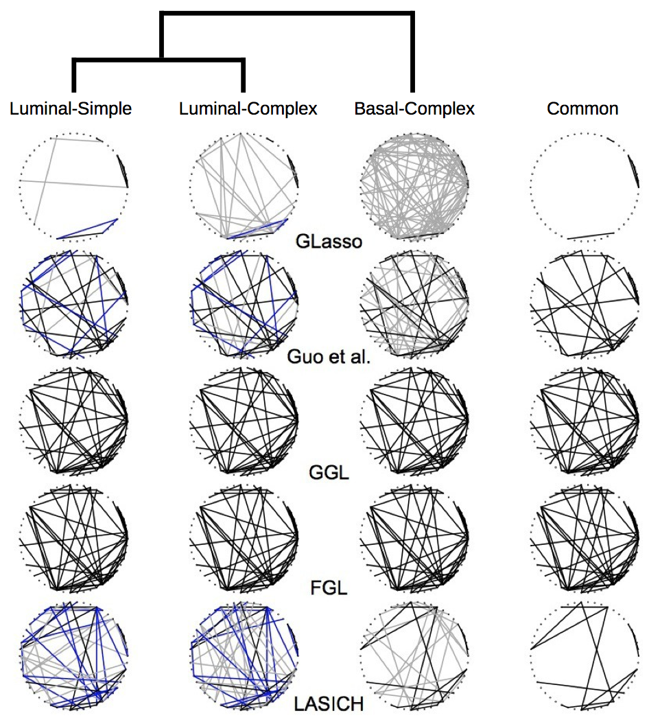
Breast cancer is heterogenous with multiple clinically verified subtypes (Perou et al., 2000). Jönsson et al. (2010) used copy number variation and gene expression measurements to identify new subtypes of breast cancer and showed that the identified subtypes have distinct clinical outcomes. The genetic networks of these different subtypes are expected to share similarities, but to also have unique features. Moreover, the similarities among the networks are expected to corroborate with the clustering of the subtypes based on their molecular profiles. We applied network estimation methods of Section 6.1 to a subset of the microarray gene expression data from Jönsson et al. (2010), containing data for 218 patients classified into three previously known subtypes of breast cancer: 46 Luminal-simple, 105 Luminal-complex and 67 Basal-complex samples. For ease of presentation, we focused on 50 genes with largest variances. The hierarchical clustering results of Jönsson et al. (2010), reproduced in Figure 5 for the above three subtypes, were used to identify the subpopulation membership; reciprocals of distances in the dendrogram were used to define similarities among subtypes used in the graph Laplacian penalty.

To facilitate the comparison, tuning parameters were selected such that the estimated networks of the three subtypes using each method contained a total of 150 edges. For methods with two tuning parameters, pairs of tuning parameters were determined using the Bayesian information criterion (BIC), as described in Guo et al. (2011). Estimated genetic networks of the three cancer subtypes are shown in Figure 5. For each method, edges common in all three subtypes, those common in Luminal subtypes and subtype specific edges are distinguished.

In this example, results from separate graphical lasso estimation and FGL/GGL are two extremes. Estimated network topologies from graphical lasso vary from subtype to subtype, and common structures are obscured; this variability may be because similarities among subtypes are not incorporated in the estimation. In contrast, FGL and GGL give identical networks for all subtypes, perhaps because both methods encourage the estimated networks of all subtypes to be equally similar. Intermediate results are obtained using LASICH and the method of Guo et al. (2011). The main difference between these two methods is that Guo et al. (2011) finds more edges common to all three subtypes, whereas LASICH finds more edges common to the Luminal subtypes. This difference is likely because LASICH prioritizes the similarity between the Luminal subtypes via graph Laplacian while the method of Guo et al. (2011) does not distinguish between the three subtypes. The above example highlights the potential advantages of LASICH in providing network estimates that better corroborate with the known hierarchy of subpopulations.
Refer to caption
Figure 5: Dendrogram of hierarchical clustering of three subtypes of breast cancer from Jönsson et al. (2010) along with estimated gene networks using graphical lasso (Glasso), method of Guo et al., FGL and GGL of Daneher et al. (2014) and LASICH. Blue edges are common to Luminal subtypes and black edges are shared by all three subtypes; condition specific edges are drawn in gray.

7 Discussion

We introduced a flexible method for joint estimation of multiple precision matrices, called LASICH, which is particularly suited for settings where observations belong to three or more subpopulations. In the proposed method, the relationships among heterogenous subpopulations is captured by a weighted network, whose nodes correspond to subpopulations, and whose edges capture their similarities. As a result, LASICH can model complex relationships among subpopulations, defined, for example, based on hierarchical clustering of samples.

We established asymptotic properties of the proposed estimator in the setting where the relationship among subpopulations is externally defined. We also extended the method to the setting of unknown relationships among subpopulations, by showing that clusters estimated from the data can accurately capture the true relationships. The proposed method generalizes existing convex penalties for joint estimation of graphical models, and can be particularly advantageous in settings with multiple subpopulations.

A particularly appealing feature of the proposed extension of LASICH is that it can also be applied in settings where the subpopulation memberships are unknown. The latter setting is closely related to estimation of precision matrices for mixture of Gaussian distributions. Both approaches have limitations and drawbacks: on the one hand, the extension of LASICH to unknown subpopulation memberships requires certain assumptions on differences of population means (Section 4). On the other hand, estimation of precision matrices for mixture of Gaussians is computationally challenging, and known rates of convergence of parameter estimation in mixture distributions (e.g. in Städler et al. (2010)) are considerably slower.

Throughout this paper we assumed that the number of subpopulations is known. Extensions of this method to estimation of graphical models in populations with an unknown number of subpopulations would be particularly interesting for analysis of genetic networks associated with heterogeneity in cancer samples, and are left for future research.

8 Appendix: Proofs and Technical Detials

We denote true inverse correlation matrices as Θ0=(Θ0(1),…,Θ0(K))\Theta_{0}=(\Theta^{(1)}_{0},\ldots,\Theta_{0}^{(K)}) and true correlation matrices as Ψ0=(Ψ0(1),…,Ψ0(K))\Psi_{0}=(\Psi^{(1)}_{0},\ldots,\Psi_{0}^{(K)}), where Θ0(k)≡(Ψ0(k))−1≡(θ0,i​j(k))i,j=1p\Theta_{0}^{(k)}\equiv(\Psi_{0}^{(k)})^{-1}\equiv(\theta^{(k)}_{0,ij})_{i,j=1}^{p}, and Ψ0(k)=(ψ0,i​j(k))i,j=1p\Psi_{0}^{(k)}=(\psi_{0,ij}^{(k)})_{i,j=1}^{p}. The estimates of the population parameters are dented as Σ^n(k)=(σ^i​j)i,j=1p\hat{\Sigma}^{(k)}_{n}=(\hat{\sigma}_{ij})_{i,j=1}^{p}, Ψn(k)=(ψn,i​j)i,j=1p\Psi^{(k)}_{n}=(\psi_{n,ij})_{i,j=1}^{p}, and Θ^ρn(k)=(θ^ρn,i​j(k))i,j=1p\hat{\Theta}^{(k)}_{\rho_{n}}=(\hat{\theta}_{\rho_{n},ij}^{(k)})_{i,j=1}^{p}. For a vector x=(x1,…,xp)Tx=(x_{1},\ldots,x_{p})^{T} and J⊂{1,…,p}J\subset\{1,\ldots,p\}, we denote xJ=(xj,j∈J)Tx_{J}=(x_{j},j\in J)^{T}. For a matrix AA, λk​(A)\lambda_{k}(A) is the kkth smallest eigenvalue and A→\vec{A} is the vectorization of AA. For J⊂{(i,j):i,j=1,…,p}J\subset\{(i,j):i,j=1,\ldots,p\} and A∈ℝp×pA\in\mathbb{R}^{p\times p}, A→J\vec{A}_{J} is a vector in ℝ|J|\mathbb{R}^{|J|} obtained by removing elements corresponding to (i,j)∉J(i,j)\notin J from A→\vec{A}. A zero-filled matrix AJ∈ℝp×pA_{J}\in\mathbb{R}^{p\times p} is obtained from AA by replacing ai​ja_{ij} by 0 for (i,j)∉J(i,j)\notin J.

8.1 Consistency in Matrix Norms

Theorem 1 is a direct consequence of the following result.

Lemma 1.

(i) Suppose that Condition 1 holds. Let γ∈(0,mink⁡πk)\gamma\in(0,\min_{k}\pi_{k}) be arbitrary. For

n≥max⁡{6​γ−1​log​p, 215​33​C12​γ−3​(1+4​c12)2​maxk,i​{σi​i(k)}2​λΘ4​(1+ρ2​∥L∥21/2)2​s​log​p}n\geq\max\left\{6\gamma^{-1}\log p,\,2^{15}3^{3}C_{1}^{2}\gamma^{-3}(1+4c_{1}^{2})^{2}\max_{k,i}\{\sigma_{ii}^{(k)}\}^{2}\lambda_{\Theta}^{4}\left(1+\rho_{2}\lVert L\rVert_{2}^{1/2}\right)^{2}s\log p\right\}

and ρn=236C1(1+4c12)γ−1/2maxk,iσi​i(k)log⁡p/n\rho_{n}=2^{3}\sqrt{6}C_{1}(1+4c_{1}^{2})\gamma^{-1/2}\max_{k,i}\sigma_{ii}^{(k)}\sqrt{\log p/n}, we have with probability (1−2​K/p)​(1−2​K​exp⁡(−2​n​(mink⁡πk−γ)2))(1-2K/p)(1-2K\exp(-2n(\min_{k}\pi_{k}-\gamma)^{2})) that

∑k=1K∥Θ^ρn(k)−Θ0(k)∥F≤215/233/2C1γ−3/2(1+4c12)maxk,iσi​i(k)λΘ2(1+ρ2∥L∥21/2)s​log⁡pn.\displaystyle\sum_{k=1}^{K}\lVert\hat{\Theta}_{\rho_{n}}^{(k)}-\Theta_{0}^{(k)}\rVert_{F}\leq 2^{15/2}3^{3/2}C_{1}\gamma^{-3/2}(1+4c_{1}^{2})\max_{k,i}\sigma_{ii}^{(k)}\lambda_{\Theta}^{2}\left(1+\rho_{2}\lVert L\rVert_{2}^{1/2}\right)\sqrt{\frac{s\log p}{n}}.

(ii) Suppose that Condition 2 holds with p≤c7​nc2p\leq c_{7}n^{c_{2}}, c2,c3,c7>0c_{2},c_{3},c_{7}>0. For ρn=C1​K​δn\rho_{n}=C_{1}K\delta_{n} satisfying

24​32​C1​ρn2​γ−2​s​(1+ρ2​∥L∥21/2)2​λΘ4≤1/42^{4}3^{2}C_{1}\rho_{n}^{2}\gamma^{-2}s(1+\rho_{2}\lVert L\rVert_{2}^{1/2})^{2}\lambda_{\Theta}^{4}\leq 1/4

and τ>(27+23​1+24​32​c4​maxk,i​{σi​i(k)}2)/(9​c4​maxk,i​{σi​i(k)}2)\tau>(2^{7}+2^{3}\sqrt{1+2^{4}3^{2}c_{4}\max_{k,i}\{\sigma_{ii}^{(k)}\}^{2}})/(9c_{4}\max_{k,i}\{\sigma_{ii}^{(k)}\}^{2}) we have with probability (1−2​K​exp⁡(−2​n​(mink⁡πk−γ)2))​νn(1-2K\exp(-2n(\min_{k}\pi_{k}-\gamma)^{2}))\nu_{n} that

∑k=1K∥Θ^ρn(k)−Θ0(k)∥F≤24​33/2​C1​γ−2​K​(1+ρ2​∥L∥21/2)​λΘ2​s1/2​δn,\displaystyle\sum_{k=1}^{K}\lVert\hat{\Theta}_{\rho_{n}}^{(k)}-\Theta_{0}^{(k)}\rVert_{F}\leq 2^{4}3^{3/2}C_{1}\gamma^{-2}K\left(1+\rho_{2}\lVert L\rVert_{2}^{1/2}\right)\lambda_{\Theta}^{2}s^{1/2}\delta_{n},

where

δn\displaystyle\delta_{n} ≡\displaystyle\equiv maxk,i⁡{σi​i(k)}2​c4​(4+τ)​γ−1​log⁡pn+(1+2​maxk,i​|μ(k),i|)​maxk,i⁡{σi​i(k)}2​c4​(4+τ)​γ−1​log⁡pn\displaystyle\max_{k,i}\{\sigma_{ii}^{(k)}\}^{2}c_{4}(4+\tau)\gamma^{-1}\frac{\log p}{n}+(1+2\max_{k,i}|\mu^{(k),i}|)\sqrt{\max_{k,i}\{\sigma_{ii}^{(k)}\}^{2}c_{4}(4+\tau)\gamma^{-1}\frac{\log p}{n}}
+2​maxk,i,j⁡𝔼|X(k),i​X(k),j|​I​(|X(k),i​X(k),j|≥γ​nlog⁡p)+4​{maxk,i⁡𝔼|X(k),i|​I​(|X(k),i|≥γ​nlog⁡p)}2\displaystyle+2\max_{k,i,j}\E|X^{(k),i}X^{(k),j}|I\left(|X^{(k),i}X^{(k),j}|\geq\sqrt{\frac{\gamma n}{\log p}}\right)+4\left\{\max_{k,i}\E|X^{(k),i}|I\left(|X^{(k),i}|\geq\sqrt{\frac{\gamma n}{\log p}}\right)\right\}^{2}
+2​(1+2​maxk,i​|μ(k),i|)​maxk,i⁡𝔼|X(k),i|​I​(|X(k),i|≥γ​nlog⁡p)\displaystyle+2(1+2\max_{k,i}|\mu^{(k),i}|)\max_{k,i}\E|X^{(k),i}|I\left(|X^{(k),i}|\geq\sqrt{\frac{\gamma n}{\log p}}\right)
=O⁡(log⁡pn),\displaystyle=O\left(\sqrt{\frac{\log p}{n}}\right),

and

νn\displaystyle\nu_{n} ≡\displaystyle\equiv 3​c7​c4​maxk,i​{σi​i(k)}2​(log⁡p)c2+c3+1γc3​nc3+c7​c4​maxk,i​σi​i(k)​(log⁡p)2​(c2+c3+1)nc2+c3+1\displaystyle\frac{3c_{7}c_{4}\max_{k,i}\{\sigma_{ii}^{(k)}\}^{2}(\log p)^{c_{2}+c_{3}+1}}{\gamma^{c_{3}}n^{c_{3}}}+\frac{c_{7}c_{4}\max_{k,i}\sigma_{ii}^{(k)}(\log p)^{2(c_{2}+c_{3}+1)}}{n^{c_{2}+c_{3}+1}}
+8​p2​exp⁡(−maxk,i⁡σi​i(k)​c4​(4+τ)​log​p2​maxk,i​σi​i(k)​c4+maxk,i⁡{σi​i(k)}2​c4​(64+16​τ)/3)\displaystyle+8p^{2}\exp\left(-\frac{\max_{k,i}\sigma_{ii}^{(k)}c_{4}(4+\tau)\log p}{2\max_{k,i}\sigma_{ii}^{(k)}c_{4}+\sqrt{\max_{k,i}\{\sigma_{ii}^{(k)}\}^{2}c_{4}(64+16\tau)}/3}\right)
=o⁡(1).\displaystyle=o(1).

Our proofs adopt several tools from Negahban et al. (2012a). Note however that our penalty does not penalize the diagonal elements, and is hence a seminorm; thus, their results do not apply to our case. We first introduce several notations. To treat multiple precision matrices in a unified way, our parameter space is defined to be the set ℝ~(p​K)×(p​K)\tilde{\mathbb{R}}^{(pK)\times(pK)} of (p​K)×(p​K)(pK)\times(pK) symmetric block diagonal matrices, where the kkth diagonal block is a p×pp\times p matrix corresponding to the precision matrix of subpopulation kk. We write A∈ℝ~(p​K)×(p​K)A\in\tilde{\mathbb{R}}^{(pK)\times(pK)} for a KK-tuple (A(k))k=1K(A^{(k)})_{k=1}^{K} of diagonal blocks A(k)∈ℝp×pA^{(k)}\in\mathbb{R}^{p\times p}. Note that for A,B∈ℝ~(p​K)×(p​K)A,B\in\tilde{\mathbb{R}}^{(pK)\times(pK)}, ⟨A,B⟩p​K=∑k=1K⟨A(k),B(k)⟩p\langle A,B\rangle_{pK}=\sum_{k=1}^{K}\langle A^{(k)},B^{(k)}\rangle_{p} where ⟨⋅,⋅⟩p\langle\cdot,\cdot\rangle_{p} is the trace inner product on ℝp×p\mathbb{R}^{p\times p}. In this parameter space, we evaluate the following map from ℝ~(p​K)×(p​K)\tilde{\mathbb{R}}^{(pK)\times(pK)} to ℝ\mathbb{R} given by

f⁡(Δ)=−ℓ~n​(Θ0+Δ)+ℓ~n​(Θ0)+ρn​{r⁡(Θ0+Δ)−r⁡(Θ0)},f(\Delta)=-\tilde{\ell}_{n}(\Theta_{0}+\Delta)+\tilde{\ell}_{n}(\Theta_{0})+\rho_{n}\{r(\Theta_{0}+\Delta)-r(\Theta_{0})\},

where r:ℝ~(p​K)×(p​K)↦ℝr:\tilde{\mathbb{R}}^{(pK)\times(pK)}\mapsto\mathbb{R} is given by r⁡(Θ)=∥Θ∥1+ρ2​∥Θ∥Lr(\Theta)=\lVert\Theta\rVert_{1}+\rho_{2}\lVert\Theta\rVert_{L}. This map provides information on the behavior of our criterion function in the neighborhood of Θ0\Theta_{0}. A similar map with a different penalty was studied in Rothman et al. (2008). A key observation is that f⁡(0)=0f(0)=0 and f⁡(Δ^n)≤0f(\hat{\Delta}_{n})\leq 0 where Δ^n=Θ^ρn−Θ0\hat{\Delta}_{n}=\hat{\Theta}_{\rho_{n}}-\Theta_{0}.

The following lemma provides a non-asymptotic bound on the Frobenius norm of Δ\Delta (see Lemma 4 in Negahban et al. (2012b) for a similar lemma in a different context). Let S=∪k=1KS(k)S=\cup_{k=1}^{K}S^{(k)} be the union of the supports of Ω0(k)\Omega_{0}^{(k)}. Define a model subspace ℳ={Ω∈ℝ~(p​K)×(p​K):ωi​j(k)=0,(i,j)∉S,k=1,…,K}\mathcal{M}=\{\Omega\in\tilde{\mathbb{R}}^{(pK)\times(pK)}:\omega_{ij}^{(k)}=0,(i,j)\notin S,k=1,\ldots,K\} and its orthocomplement ℳ⟂={Ω∈ℝ~(p​K)×(p​K):ωi​j(k)=0,(i,j)∈S,k=1,…K}\mathcal{M}^{\perp}=\{\Omega\in\tilde{\mathbb{R}}^{(pK)\times(pK)}:\omega_{ij}^{(k)}=0,(i,j)\in S,k=1,\ldots K\} under the trace inner product in ℝ~(p​K)×(p​K)\tilde{\mathbb{R}}^{(pK)\times(pK)}. For A=(ai​j)i,j=1p​K∈ℝ~(p​K)×(p​K)A=(a_{ij})_{i,j=1}^{pK}\in\tilde{\mathbb{R}}^{(pK)\times(pK)}, we write A=Aℳ+Aℳ⟂A=A_{\mathcal{M}}+A_{\mathcal{M}^{\perp}} where AℳA_{\mathcal{M}} and Aℳ⟂A_{\mathcal{M}^{\perp}} are the projection of AA into ℳ\mathcal{M} and ℳ⟂\mathcal{M}^{\perp}, in the Frobenius norm, respectively. In other words, the (i,j)(i,j)-element of AℳA_{\mathcal{M}} is ai​ja_{ij} if (i,j)∈S(i,j)\in S and zero otherwise, and the (i,j)(i,j)-element of Aℳ⟂A_{\mathcal{M}^{\perp}} is ai​ja_{ij} if (i,j)∉S(i,j)\notin S and zero otherwise. Note that Θ0∈ℳ\Theta_{0}\in\mathcal{M}. Define the set 𝒞={Δ∈ℝ~(p​K)×(p​K):r⁡(Δℳ⟂)≤3​r​(Δℳ)}\mathcal{C}=\{\Delta\in\tilde{\mathbb{R}}^{(pK)\times(pK)}:r(\Delta_{\mathcal{M}^{\perp}})\leq 3r(\Delta_{\mathcal{M}})\}.

Lemma 2.

Let ϵ>0\epsilon>0 be arbitrary. Suppose ρn≥2​max1≤k≤K​∥Ψ^n(k)−Ψ0(k)∥∞\rho_{n}\geq 2\max_{1\leq k\leq K}\lVert\hat{\Psi}_{n}^{(k)}-\Psi_{0}^{(k)}\rVert_{\infty}. If f⁡(Δ)>0f(\Delta)>0 for all elements Δ∈𝒞∩{Δ∈ℝ~(p​K)×(p​K):∥Δ∥F=ϵ}\Delta\in\mathcal{C}\cap\{\Delta\in\tilde{\mathbb{R}}^{(pK)\times(pK)}:\lVert\Delta\rVert_{F}=\epsilon\} then ∥Δ^n∥F≤ϵ\lVert\hat{\Delta}_{n}\rVert_{F}\leq\epsilon.

Proof.

We first show that Δ^n∈𝒞\hat{\Delta}_{n}\in\mathcal{C}. We have by the convexity of −ℓ~n​(Θ)-\tilde{\ell}_{n}(\Theta) that

−ℓ~n​(Θ0+Δ^n)+ℓ~n​(Θ0)≥−|⟨−∇ℓ~n​(Θ0),Δ^n⟩|.-\tilde{\ell}_{n}(\Theta_{0}+\hat{\Delta}_{n})+\tilde{\ell}_{n}(\Theta_{0})\geq-|\langle-\nabla\tilde{\ell}_{n}(\Theta_{0}),\hat{\Delta}_{n}\rangle|.

It follows from Lemma 3(iv) with our choice ρn\rho_{n} that the right hand side of the inequality is further bounded below by −2−1​ρn​(r⁡(Δ^n,ℳ)+r⁡(Δ^n,ℳ⟂))-2^{-1}\rho_{n}\left(r(\hat{\Delta}_{n,\mathcal{M}})+r(\hat{\Delta}_{n,\mathcal{M}^{\perp}})\right). Applying Lemma 3(iii), we obtain

0\displaystyle 0 ≥\displaystyle\geq f⁡(Δ^n)=−ℓ~n​(Θ0+Δ^n)+ℓ~n​(Θ0)+r⁡(Θ0+Δ^n)−r⁡(Θ0)\displaystyle f(\hat{\Delta}_{n})=-\tilde{\ell}_{n}(\Theta_{0}+\hat{\Delta}_{n})+\tilde{\ell}_{n}(\Theta_{0})+r(\Theta_{0}+\hat{\Delta}_{n})-r(\Theta_{0})
≥\displaystyle\geq ρn2​r​(Δ^n,ℳ⟂)−3​ρn2​r​(Δ^n,ℳ),\displaystyle\frac{\rho_{n}}{2}r(\hat{\Delta}_{n,\mathcal{M}^{\perp}})-\frac{3\rho_{n}}{2}r(\hat{\Delta}_{n,\mathcal{M}}),

or r⁡(Δ^n,ℳ⟂)≤3​r​(Δ^n,ℳ)r(\hat{\Delta}_{n,\mathcal{M}^{\perp}})\leq 3r(\hat{\Delta}_{n,\mathcal{M}}). This verifies Δ^n∈𝒞\hat{\Delta}_{n}\in\mathcal{C}. Note that ff, as a function of Δ\Delta is sum of two convex functions ℓn\ell_{n} and rr, and is hence convex. Thus, the rest of the proof follows exactly as Lemma 4 in Negahban et al. (2012b). ∎

Lemma 3.

Let Δ∈ℝ~(p​K)×(p​K)\Delta\in\tilde{\mathbb{R}}^{(pK)\times(pK)}.

(i) The gradient of ℓ~n​(Θ0)\tilde{\ell}_{n}(\Theta_{0}) is a block diagonal matrix given by

∇ℓ~n(Θ0)=n−1diag{n1(Ψ0(1)−Ψ^n(1)),…,nK(Ψ0(K)−Ψ^n(K))}.\displaystyle\nabla\tilde{\ell}_{n}(\Theta_{0})=n^{-1}\operatornamewithlimits{diag}\{n_{1}(\Psi_{0}^{(1)}-\hat{\Psi}_{n}^{(1)}),\ldots,n_{K}(\Psi_{0}^{(K)}-\hat{\Psi}_{n}^{(K)})\}. (12)

(ii) Let c>0c>0 be a constant. For ∥Δ∥F≤c\lVert\Delta\rVert_{F}\leq c and nk/n≥γ>0n_{k}/n\geq\gamma>0 for all kk and nn,

−ℓ~n​(Θ0+Δ)+ℓ~n​(Θ0)+⟨∇ℓ~n​(Θ0),Δ⟩≥γ2​{λΘ+c}2​∥Δ∥F2≡κℓn,c​∥Δ∥F2.\displaystyle-\tilde{\ell}_{n}(\Theta_{0}+\Delta)+\tilde{\ell}_{n}(\Theta_{0})+\langle\nabla\tilde{\ell}_{n}(\Theta_{0}),\Delta\rangle\geq\frac{\gamma}{2\left\{\lambda_{\Theta}+c\right\}^{2}}\lVert\Delta\rVert_{F}^{2}\equiv\kappa_{\ell_{n},c}\lVert\Delta\rVert_{F}^{2}. (13)

(iii) The map rr is a seminorm, convex, and decomposable with respect to (ℳ,ℳ⟂)(\mathcal{M},\mathcal{M}^{\perp}) in the sense that r⁡(Θ1+Θ2)=r⁡(Θ1)+r⁡(Θ2)r(\Theta_{1}+\Theta_{2})=r(\Theta_{1})+r(\Theta_{2}) for every Θ1∈ℳ\Theta_{1}\in\mathcal{M} and Θ2∈ℳ⟂\Theta_{2}\in\mathcal{M}^{\perp}. Moreover,

r⁡(Θ0+Δ)−r⁡(Θ0)≥r⁡(Δℳ⟂)−r⁡(Δℳ).r(\Theta_{0}+\Delta)-r(\Theta_{0})\geq r(\Delta_{\mathcal{M}^{\perp}})-r(\Delta_{\mathcal{M}}).

(iv) For Δ∈ℝ~(p​K)×(p​K)\Delta\in\tilde{\mathbb{R}}^{(pK)\times(pK)},

|⟨∇ℓ~n​(Θ0),Δ⟩|≤r⁡(Δ)​max1≤k≤K​∥Ψ^n(k)−Ψ0(k)∥∞.|\langle\nabla\tilde{\ell}_{n}(\Theta_{0}),\Delta\rangle|\leq r(\Delta)\max_{1\leq k\leq K}\lVert\hat{\Psi}_{n}^{(k)}-\Psi_{0}^{(k)}\rVert_{\infty}. (14)

(v) For Θ∈ℝ~(p​K)×(p​K)\Theta\in\tilde{\mathbb{R}}^{(pK)\times(pK)},

r⁡(Θℳ)≤(s+1)1/2​(1+ρ2​∥L∥21/2)​∥Θℳ∥F.r(\Theta_{\mathcal{M}})\leq(s+1)^{1/2}\left(1+\rho_{2}\lVert L\rVert_{2}^{1/2}\right)\lVert\Theta_{\mathcal{M}}\rVert_{F}.
Proof.

(i) The result follows by taking derivatives blockwise.

(ii) Rothman et al. (2008) (page 500-502) showed that

−ℓ~n​(Θ0+Δ)+ℓ~n​(Θ0)−⟨−∇ℓ~n​(Θ0),Δ⟩\displaystyle-\tilde{\ell}_{n}(\Theta_{0}+\Delta)+\tilde{\ell}_{n}(\Theta_{0})-\langle-\nabla\tilde{\ell}_{n}(\Theta_{0}),\Delta\rangle
=∑k=1Knkn​(−log⁡det​(Θ0(k)+Δ(k))+log⁡det​(Θ0(k))+⟨Ψ0(k),Δ(k)⟩)\displaystyle=\sum_{k=1}^{K}\frac{n_{k}}{n}\left(-\log\mbox{det}(\Theta_{0}^{(k)}+\Delta^{(k)})+\log\mbox{det}(\Theta_{0}^{(k)})+\langle\Psi_{0}^{(k)},\Delta^{(k)}\rangle\right)
≥∑k=1Knkn​∥Δ(k)∥F22​min0≤v≤1​{‖Θ0(k)‖2+v​‖Δ(k)‖2}2.\displaystyle\geq\sum_{k=1}^{K}\frac{n_{k}}{n}\frac{\lVert\Delta^{(k)}\rVert_{F}^{2}}{2\min_{0\leq v\leq 1}\left\{\left\lVert\Theta_{0}^{(k)}\right\rVert_{2}+v\left\lVert\Delta^{(k)}\right\rVert_{2}\right\}^{2}}.

Since ∥A∥2≤∥A∥F\lVert A\rVert_{2}\leq\lVert A\rVert_{F}, nk/n≥γn_{k}/n\geq\gamma and ∥Δ∥F≤c\lVert\Delta\rVert_{F}\leq c, this is further bounded below by

∑k=1Kγ2​∥Δ(k)∥F2{∥Θ0(k)∥2+‖Δ(k)‖F}2≥κℓn,c​∥Δ∥F2.\displaystyle\sum_{k=1}^{K}\frac{\gamma}{2}\frac{\lVert\Delta^{(k)}\rVert_{F}^{2}}{\left\{\lVert\Theta_{0}^{(k)}\rVert_{2}+\left\lVert\Delta^{(k)}\right\rVert_{F}\right\}^{2}}\geq\kappa_{\ell_{n},c}\lVert\Delta\rVert_{F}^{2}.

(iii) Because the graph Laplacian LL is a positive semidefinite matrix, the triangle inequality r⁡(Θ1+Θ2)≤r⁡(Θ1)+r⁡(Θ2)r(\Theta_{1}+\Theta_{2})\leq r(\Theta_{1})+r(\Theta_{2}) holds. To see this let L=L~​L~TL=\tilde{L}\tilde{L}^{T} be any Cholesky decomposition of LL. Then

{(x+y)T​L​(x+y)}1/2=∥L~T​(x+y)∥≤∥L~T​x∥+∥L~​y∥={xT​L​x}1/2+{yT​L​y}1/2.\{(x+y)^{T}L(x+y)\}^{1/2}=\lVert\tilde{L}^{T}(x+y)\rVert\leq\lVert\tilde{L}^{T}x\rVert+\lVert\tilde{L}y\rVert=\{x^{T}Lx\}^{1/2}+\{y^{T}Ly\}^{1/2}.

It is clear that r⁡(c​Θ)=c​r​(Θ)r(c\Theta)=cr(\Theta) for any constant cc. Thus, given that rr does not penalize the diagonal elements, it is a seminorm. The decomposability follows from the definition of rr. The convexity follows from the same argument for the triangle inequality. Since Θ0+Δ=Θ0+Δℳ+Δℳ⟂\Theta_{0}+\Delta=\Theta_{0}+\Delta_{\mathcal{M}}+\Delta_{\mathcal{M}^{\perp}}, the triangle inequality and the decomposability of rr yield

r⁡(Θ0+Δ)−r⁡(Θ0)≥r⁡(Θ0+Δℳ⟂)−r⁡(Δℳ)−r⁡(Θ0)=r⁡(Δℳ⟂)−r⁡(Δℳ).\displaystyle r(\Theta_{0}+\Delta)-r(\Theta_{0})\geq r(\Theta_{0}+\Delta_{\mathcal{M}^{\perp}})-r(\Delta_{\mathcal{M}})-r(\Theta_{0})=r(\Delta_{\mathcal{M}^{\perp}})-r(\Delta_{\mathcal{M}}).

(iv) We show that, for A,B∈ℝ~(p​K)×(p​K)A,B\in\tilde{\mathbb{R}}^{(pK)\times(pK)} with diag(B)=0\operatornamewithlimits{diag}(B)=0, ⟨A,B⟩≤r⁡(A)​∥B∥∞\langle A,B\rangle\leq r(A)\lVert B\rVert_{\infty}. If AA is a diagonal matrix (or if A=0A=0), the inequality trivially holds since ⟨A,B⟩=0\langle A,B\rangle=0. If not, r⁡(A)≠0r(A)\neq 0 so that

⟨A,B⟩r⁡(A)≤∥A∥1​∥B∥∞∥A∥1=∥B∥∞.\displaystyle\frac{\langle A,B\rangle}{r(A)}\leq\frac{\lVert A\rVert_{1}\lVert B\rVert_{\infty}}{\lVert A\rVert_{1}}=\lVert B\rVert_{\infty}.

Since the diagonal elements of ∇ℓ~n​(Θ0)\nabla\tilde{\ell}_{n}(\Theta_{0}) are all zero, the result follows.

(v) For s≠0s\neq 0, we have

r⁡(Θℳ)∥Θℳ∥F\displaystyle\frac{r(\Theta_{\mathcal{M}})}{\lVert\Theta_{\mathcal{M}}\rVert_{F}} ≤\displaystyle\leq supΘ∈ℳ∑k=1K∥Θ(k)∥1∥Θ−diag(Θ)∥F+supΘ∈ℳρ2​∑i≠jθi​jT​L​θi​j∥Θ∥F\displaystyle\sup_{\Theta\in\mathcal{M}}\frac{\sum_{k=1}^{K}\lVert\Theta^{(k)}\rVert_{1}}{\lVert\Theta-\operatornamewithlimits{diag}(\Theta)\rVert_{F}}+\sup_{\Theta\in\mathcal{M}}\frac{\rho_{2}\sum_{i\neq j}\sqrt{\theta_{ij}^{T}L\theta_{ij}}}{\lVert\Theta\rVert_{F}}
≤\displaystyle\leq s1/2+ρ2​supΘ∈ℳ∑i≠j∥L∥2​∥θi​j∥F2∥Θ∥F\displaystyle s^{1/2}+\rho_{2}\sup_{\Theta\in\mathcal{M}}\frac{\sum_{i\neq j}\sqrt{\lVert L\rVert_{2}\lVert\theta_{ij}\rVert_{F}^{2}}}{\lVert\Theta\rVert_{F}}
≤\displaystyle\leq s1/2​(1+ρ2​∥L∥21/2).\displaystyle s^{1/2}\left(1+\rho_{2}\lVert L\rVert_{2}^{1/2}\right).

In the last inequality we used the fact that ∑j=1J∑i=1Iai​j2≥J−1/2∑j=1J∑i=1Iai​j2\sqrt{\sum_{j=1}^{J}\sum_{i=1}^{I}a_{ij}^{2}}\geq J^{-1/2}\sum_{j=1}^{J}\sqrt{\sum_{i=1}^{I}a_{ij}^{2}}, which follows by the concavity of the square root function. For s=0s=0, we trivially have 0=r⁡(Θℳ)≤s1/2​{1+ρ2​∥L∥21/2}​∥Θℳ∥F0=r(\Theta_{\mathcal{M}})\leq s^{1/2}\{1+\rho_{2}\lVert L\rVert_{2}^{1/2}\}\lVert\Theta_{\mathcal{M}}\rVert_{F}. Combining these two cases yields the desired result. ∎

Next, we obtain an upper bound for max1≤k≤K⁡∥Ψ^n(k)−Ψ0(k)∥∞\max_{1\leq k\leq K}\lVert\hat{\Psi}_{n}^{(k)}-\Psi_{0}^{(k)}\rVert_{\infty}, which holds with high-probability assuming the tail conditions of the random vectors.

Lemma 4.

Suppose that nk/n≥γ>0n_{k}/n\geq\gamma>0 for all kk and nn.

(i) Suppose that Condition 1 holds. Then for n≥6​γ−1​log⁡pn\geq 6\gamma^{-1}\log p we have

P(∥Σ^n−Σ0∥∞≥236(1+4c12)2γ−1/2maxk,iσi​i(k)log⁡pγ​n)≤2K/p.\displaystyle P\left(\lVert\hat{\Sigma}_{n}-\Sigma_{0}\rVert_{\infty}\geq 2^{3}\sqrt{6}(1+4c_{1}^{2})^{2}\gamma^{-1/2}\max_{k,i}\sigma^{(k)}_{ii}\sqrt{\frac{\log p}{\gamma n}}\right)\leq 2K/p. (15)

(ii) Suppose that Condition 2 holds with c2,c3>0c_{2},c_{3}>0 and p≤c7​nc2p\leq c_{7}n^{c_{2}}. Then we have for τ>maxk(27+231+2432c4maxk,i{σi​i(k)}2)/(9c4maxk,i{σi​i(k)}2)\tau>\max_{k}(2^{7}+2^{3}\sqrt{1+2^{4}3^{2}c_{4}\max_{k,i}\{\sigma_{ii}^{(k)}}\}^{2})/(9c_{4}\max_{k,i}\{\sigma_{ii}^{(k)}\}^{2})

P⁡(∥Σ^n−Σ0∥∞≥∑k=1Kδn(k))≤K​νn\displaystyle P\left(\lVert\hat{\Sigma}_{n}-\Sigma_{0}\rVert_{\infty}\geq\sum_{k=1}^{K}\delta_{n}^{(k)}\right)\leq K\nu_{n} (16)

where

δn(k)≡(1+2​maxi​|μ(k),i|)​(2​δn,1(k)+δn,2(k))+(δn,1(k))2+(δn,2(k))2+2​δn,3(k),\displaystyle\delta_{n}^{(k)}\equiv(1+2\max_{i}|\mu^{(k),i}|)(2\delta_{n,1}^{(k)}+\delta_{n,2}^{(k)})+(\delta_{n,1}^{(k)})^{2}+(\delta_{n,2}^{(k)})^{2}+2\delta_{n,3}^{(k)},

with

δn,1(k)≡maxi,j𝔼|Xl(k),iXl(k),j|I(|Xl(k),iXl(k),j|≥nk1/2(logp)−1/2),\displaystyle\delta_{n,1}^{(k)}\equiv\max_{i,j}\E|X^{(k),i}_{l}X^{(k),j}_{l}|I(|X^{(k),i}_{l}X^{(k),j}_{l}|\geq n_{k}^{1/2}(\log p)^{-1/2}),
δn,2(k)≡{c4​maxk,i​{σi​i(k)}2​(4+τ)​log⁡p/nk}1/2,\displaystyle\delta_{n,2}^{(k)}\equiv\{c_{4}\max_{k,i}\{\sigma_{ii}^{(k)}\}^{2}(4+\tau)\log p/n_{k}\}^{1/2},
δn,3(k)≡maxi𝔼|Xl(k),i|I(|Xl(k),i|≥nk1/2(logp)−1/2).\displaystyle\delta_{n,3}^{(k)}\equiv\max_{i}\E|X^{(k),i}_{l}|I(|X^{(k),i}_{l}|\geq n_{k}^{1/2}(\log p)^{-1/2}).

(iii) Suppose that Condition 3 holds and that P⁡(∥Σ^n−Σ0∥∞≥bn)=o⁡(1)P(\lVert\hat{\Sigma}_{n}-\Sigma_{0}\rVert_{\infty}\geq b_{n})=o(1) and bn=o⁡(1)b_{n}=o(1) as n→∞n\rightarrow\infty. Then P⁡(∥Ψ^n−Ψ0∥∞≥C1​bn)=o⁡(1)P(\lVert\hat{\Psi}_{n}-\Psi_{0}\rVert_{\infty}\geq C_{1}b_{n})=o(1).

Proof.

(i) This was proved by Ravikumar et al. (2011).

(ii) Note that

Σ^n(k)−Σ(k)\displaystyle\hat{\Sigma}^{(k)}_{n}-\Sigma^{(k)} =\displaystyle= nk−1​∑l=1nk(Xl(k))⊗2−𝔼(X(k))⊗2−(X¯(k)−μ(k))⊗2\displaystyle{n_{k}}^{-1}\sum_{l=1}^{n_{k}}(X^{(k)}_{l})^{\otimes 2}-\E(X^{(k)})^{\otimes 2}-(\overline{X}^{(k)}-\mu^{(k)})^{\otimes 2}
−μ(k)​(X¯(k)−μ(k))T−(X¯(k)−μ(k))​(μ(k))T.\displaystyle-\mu^{(k)}(\overline{X}^{(k)}-\mu^{(k)})^{T}-(\overline{X}^{(k)}-\mu^{(k)})(\mu^{(k)})^{T}.

We first evaluate the probability in (16) for nk−1​∑l=1nk(Xl(k))⊗2−𝔼(X(k))⊗2n_{k}^{-1}\sum_{l=1}^{n_{k}}(X^{(k)}_{l})^{\otimes 2}-\E(X^{(k)})^{\otimes 2}. Let

Y(k),i​jl≡X(k),ilX(k),jl−𝔼X(k),ilX(k),jl,\displaystyle Y^{(k),ij}_{l}\equiv X^{(k),i}_{l}X^{(k),j}_{l}-\E X^{(k),i}_{l}X^{(k),j}_{l},
Y¯l(k),i​j≡Xl(k),iXl(k),jI(|Xl(k),iXl(k),j|≤nklog⁡p)−𝔼Xl(k),iXl(k),jI(|Xl(k),iXl(k),j|≤nklog⁡p),\displaystyle\bar{Y}^{(k),ij}_{l}\equiv X^{(k),i}_{l}X^{(k),j}_{l}I\left(|X^{(k),i}_{l}X^{(k),j}_{l}|\leq\sqrt{\frac{n_{k}}{\log p}}\right)-\E X^{(k),i}_{l}X^{(k),j}_{l}I\left(|X^{(k),i}_{l}X^{(k),j}_{l}|\leq\sqrt{\frac{n_{k}}{\log p}}\right),
Y~l(k),i​j≡Yl(k),i​j−Y¯l(k),i​j.\displaystyle\tilde{Y}^{(k),ij}_{l}\equiv Y^{(k),ij}_{l}-\bar{Y}^{(k),ij}_{l}.

We have

P⁡(maxi,j⁡|∑l=1nkY~l(k),i​j|≥2​nk​δn,1(k))\displaystyle P\left(\max_{i,j}\left|\sum_{l=1}^{n_{k}}\tilde{Y}^{(k),ij}_{l}\right|\geq 2n_{k}\delta_{n,1}^{(k)}\right)
≤P(maxi,j|∑l=1nkXl(k),iXl(k),jI(|Xl(k),iXl(k),j|≥nklog⁡p)|≥nkδn,1(k))(triangle inequality)\displaystyle\leq P\left(\max_{i,j}\left|\sum_{l=1}^{n_{k}}X^{(k),i}_{l}X^{(k),j}_{l}I\left(|X^{(k),i}_{l}X^{(k),j}_{l}|\geq\sqrt{\frac{n_{k}}{\log p}}\right)\right|\geq n_{k}\delta_{n,1}^{(k)}\right)\quad\mbox{(triangle inequality)}
≤P(maxl,i(Xl(k),i)2≥nk1/2(logp)−1/2)(xy≤max{x2,y2})\displaystyle\leq P\left(\max_{l,i}(X^{(k),i}_{l})^{2}\geq n_{k}^{1/2}(\log p)^{-1/2}\right)\quad(xy\leq\max\{x^{2},y^{2}\})
≤pnk𝔼X0​i4​(c2+c3+1)(logp)c2+c3+1nkc2+c3+1(Markov’s inequality)\displaystyle\leq pn_{k}\frac{\E X_{0i}^{4(c_{2}+c_{3}+1)}(\log p)^{c_{2}+c_{3}+1}}{n_{k}^{c_{2}+c_{3}+1}}\quad\mbox{(Markov's inequality)}
≤c7​c4​maxk,i​{σi​i(k)}2​(log⁡p)c2+c3+1nkc3(p≤c7nc2)\displaystyle\leq\frac{c_{7}c_{4}\max_{k,i}\{\sigma_{ii}^{(k)}\}^{2}(\log p)^{c_{2}+c_{3}+1}}{n_{k}^{c_{3}}}\quad(p\leq c_{7}n^{c_{2}})
≤c7​c4​maxk,i​{σi​i(k)}2​(log⁡p)c2+c3+1γc3​nc3≡νn,1.\displaystyle\leq\frac{c_{7}c_{4}\max_{k,i}\{\sigma_{ii}^{(k)}\}^{2}(\log p)^{c_{2}+c_{3}+1}}{\gamma^{c_{3}}n^{c_{3}}}\equiv\nu_{n,1}. (17)

Note that

𝔼(Y¯l(k),ij)2\displaystyle\E(\bar{Y}^{(k),ij}_{l})^{2} ≤\displaystyle\leq 𝔼[Xl(k),i​Xl(k),j​I​(|Xl(k),i​Xl(k),j|≤nklog⁡p)]2≤𝔼|Xl(k),i​Xl(k),j|2\displaystyle\E\left[X^{(k),i}_{l}X^{(k),j}_{l}I\left(|X^{(k),i}_{l}X^{(k),j}_{l}|\leq\sqrt{\frac{n_{k}}{\log p}}\right)\right]^{2}\leq\E|X^{(k),i}_{l}X^{(k),j}_{l}|^{2}
≤\displaystyle\leq 2−1​(𝔼(Xl(k),i)4+𝔼(Xl(k),j)4)≤c4​maxk,i​{σii(k)}2.\displaystyle 2^{-1}(\E(X^{(k),i}_{l})^{4}+\E(X^{(k),j}_{l})^{4})\leq c_{4}\max_{k,i}\{\sigma_{ii}^{(k)}\}^{2}.

It follows from Bernstein’s inequality that

P⁡(maxi,j⁡|∑l=1nkY¯l(k),i​j|≥nk​δn,2(k))\displaystyle P\left(\max_{i,j}\left|\sum_{l=1}^{n_{k}}\bar{Y}^{(k),ij}_{l}\right|\geq n_{k}\delta_{n,2}^{(k)}\right)
≤2​p2​exp⁡(−c4​maxk,i​{σi​i(k)}2​(4+τ)​log⁡p2​c4​maxk,i​{σi​i(k)}2+2​c4​maxk,i​{σi​i(k)}2​(64+16​τ)/3)≡νn,2.\displaystyle\leq 2p^{2}\exp\left(-\frac{c_{4}\max_{k,i}\{\sigma_{ii}^{(k)}\}^{2}(4+\tau)\log p}{2c_{4}\max_{k,i}\{\sigma_{ii}^{(k)}\}^{2}+2\sqrt{c_{4}\max_{k,i}\{\sigma_{ii}^{(k)}\}^{2}(64+16\tau)}/3}\right)\equiv\nu_{n,2}. (18)

Note that νn,2→0\nu_{n,2}\rightarrow 0 as p→∞p\rightarrow\infty for τ>(27+231+2432c4maxk,i{σi​i(k)}2)/(9c4maxk,i{σi​i(k)}2)\tau>(2^{7}+2^{3}\sqrt{1+2^{4}3^{2}c_{4}\max_{k,i}\{\sigma_{ii}^{(k)}}\}^{2})/(9c_{4}\max_{k,i}\{\sigma_{ii}^{(k)}\}^{2}). To see this note that we need to have

3​c4​maxk,i​{σi​i(k)}2​(4+τ)6​c4​maxk,i​{σi​i(k)}2+8​c4​maxk,i​{σi​i(k)}2​(4+τ)>2.\displaystyle\frac{3c_{4}\max_{k,i}\{\sigma_{ii}^{(k)}\}^{2}(4+\tau)}{6c_{4}\max_{k,i}\{\sigma_{ii}^{(k)}\}^{2}+8\sqrt{c_{4}\max_{k,i}\{\sigma_{ii}^{(k)}\}^{2}(4+\tau)}}>2.

so that the power in the exponent is strictly negative. This inequality reduces to

3​c4​maxk,i​{σi​i(k)}2​τ>16​c4​maxk,i​{σi​i(k)}2​(4+τ).\displaystyle 3c_{4}\max_{k,i}\{\sigma_{ii}^{(k)}\}^{2}\tau>16\sqrt{c_{4}\max_{k,i}\{\sigma_{ii}^{(k)}\}^{2}(4+\tau)}.

We can solve this by changing a quadratic equation for τ\tau, since τ\tau of our interest is positive. Combining (17) and (18) yields

P⁡(‖1nk​∑i=1nk(Xl(k))⊗2−𝔼(X(k))⊗2‖∞≥2​δn,1(k)+δn,2(k))≤νn,1+νn,2.\displaystyle P\left(\left\lVert\frac{1}{n_{k}}\sum_{i=1}^{n_{k}}(X^{(k)}_{l})^{\otimes 2}-\E(X^{(k)})^{\otimes 2}\right\rVert_{\infty}\geq 2\delta_{n,1}^{(k)}+\delta_{n,2}^{(k)}\right)\leq\nu_{n,1}+\nu_{n,2}. (19)

Let

Zl(k),i≡Xl(k),i−𝔼Xl(k),i,\displaystyle Z^{(k),i}_{l}\equiv X^{(k),i}_{l}-\E X_{l}^{(k),i},
Z¯l(k),i≡Xl(k),iI(|Xl(k),i|≤nk1/2(logp)−1/2)−𝔼Xl(k),iI(|Xl(k),i|≤nk1/2(logp)−1/2),\displaystyle\bar{Z}^{(k),i}_{l}\equiv X^{(k),i}_{l}I(|X^{(k),i}_{l}|\leq n_{k}^{1/2}(\log p)^{-1/2})-\E X^{(k),i}_{l}I(|X^{(k),i}_{l}|\leq n_{k}^{1/2}(\log p)^{-1/2}),
Z~l(k),i≡Ul(k),i−Z¯l(k),i.\displaystyle\tilde{Z}^{(k),i}_{l}\equiv U^{(k),i}_{l}-\bar{Z}^{(k),i}_{l}.

Proceeding as for Yl(k),i​jY^{(k),ij}_{l}’s, we have

P⁡(maxi⁡|∑l=1nkZ~l(k),i|≥2​nk​δn,3(k))≤c7​c4​maxk,i​{σi​i(k)}2​(log⁡p)2​(c2+c3+1)γc2+c3+1​nc2+c3+1≡νn,3,\displaystyle P\left(\max_{i}\left|\sum_{l=1}^{n_{k}}\tilde{Z}^{(k),i}_{l}\right|\geq 2n_{k}\delta_{n,3}^{(k)}\right)\leq\frac{c_{7}c_{4}\max_{k,i}\{\sigma_{ii}^{(k)}\}^{2}(\log p)^{2(c_{2}+c_{3}+1)}}{\gamma^{c_{2}+c_{3}+1}n^{c_{2}+c_{3}+1}}\equiv\nu_{n,3},

and

P⁡(maxi⁡|∑k=1nZ¯l(k),i|≥nk​δn,2(k))≤νn,2.\displaystyle P\left(\max_{i}\left|\sum_{k=1}^{n}\bar{Z}^{(k),i}_{l}\right|\geq n_{k}\delta_{n,2}^{(k)}\right)\leq\nu_{n,2}.

Thus, we have

P⁡(∥(X¯(k)−μ(k))⊗2∥∞≥(δn,2(k))2+(2​δn,3(k))2)≤P⁡(maxi⁡|X¯(k),i−μ(k),i|≥(δn,1(k))2+(δn,2(k))2)\displaystyle P(\lVert(\overline{X}^{(k)}-\mu^{(k)})^{\otimes 2}\rVert_{\infty}\geq(\delta_{n,2}^{(k)})^{2}+(2\delta_{n,3}^{(k)})^{2})\leq P\left(\max_{i}|\overline{X}^{(k),i}-\mu^{(k),i}|\geq\sqrt{(\delta_{n,1}^{(k)})^{2}+(\delta_{n,2}^{(k)})^{2}}\right)
≤P⁡(maxi⁡|∑k=1nZ¯l(k),i|≥nk​δn,2(k))+P⁡(maxi⁡|∑l=1nkZ~l(k),i|≥2​nk​δn,3(k))\displaystyle\leq P\left(\max_{i}\left|\sum_{k=1}^{n}\bar{Z}^{(k),i}_{l}\right|\geq n_{k}\delta_{n,2}^{(k)}\right)+P\left(\max_{i}\left|\sum_{l=1}^{n_{k}}\tilde{Z}^{(k),i}_{l}\right|\geq 2n_{k}\delta_{n,3}^{(k)}\right)
≤νn,2+νn,3,\displaystyle\leq\nu_{n,2}+\nu_{n,3}, (20)

and

P⁡(∥(X¯(k)−μ(k))​(μ(k))T∥∞≥maxi⁡|μ(k),i|​(2​δn,1(k)+δn,2(k)))\displaystyle P\left(\lVert(\overline{X}^{(k)}-\mu^{(k)})(\mu^{(k)})^{T}\rVert_{\infty}\geq\max_{i}|\mu^{(k),i}|(2\delta_{n,1}^{(k)}+\delta_{n,2}^{(k)})\right)
≤P⁡(maxi⁡|X¯(k),i−μ(k),i|≥2​δn,1(k)+δn,2(k))≤νn,1+νn,2.\displaystyle\leq P\left(\max_{i}|\overline{X}^{(k),i}-\mu^{(k),i}|\geq 2\delta_{n,1}^{(k)}+\delta_{n,2}^{(k)}\right)\leq\nu_{n,1}+\nu_{n,2}. (21)

Combining (19)-(21) yields

P⁡(∥Σ^n(k)−Σ(k)∥∞≥(1+2​maxi​|μ(k),i|)​(2​δn,1(k)+δn,2(k))+(δn,2(k))2+(2​δn,3(k))2)\displaystyle P\left(\lVert\hat{\Sigma}^{(k)}_{n}-\Sigma^{(k)}\rVert_{\infty}\geq(1+2\max_{i}|\mu^{(k),i}|)(2\delta_{n,1}^{(k)}+\delta_{n,2}^{(k)})+(\delta_{n,2}^{(k)})^{2}+(2\delta_{n,3}^{(k)})^{2}\right)
≤3​νn,1+4​νn,2+νn,3=νn.\displaystyle\leq 3\nu_{n,1}+4\nu_{n,2}+\nu_{n,3}=\nu_{n}.

Note that δn,1(k),δn,2(k),δn,3(k),νn,1,νn,2,νn,3→0\delta_{n,1}^{(k)},\delta_{n,2}^{(k)},\delta_{n,3}^{(k)},\nu_{n,1},\nu_{n,2},\nu_{n,3}\rightarrow 0 as n,p→∞n,p\rightarrow\infty if log⁡p/n→0\log p/n\rightarrow 0. Note also that δn,1(k)\delta_{n,1}^{(k)}, δn,2(k)\delta_{n,2}^{(k)} and (δn,3(k))2(\delta_{n,3}^{(k)})^{2} are O⁡(log⁡p/n)O\left(\sqrt{\log p/n}\right) on the set where nk/n≥γn_{k}/n\geq\gamma. For example, we have by Jensen’s inequality that

nlog⁡p​(δn,3(k))2\displaystyle\sqrt{\frac{n}{\log p}}(\delta_{n,3}^{(k)})^{2} =\displaystyle= nlog⁡pmaxi{𝔼|X(k),i|I{|X(k),i|≥nk1/2(logp)−1/2}}2\displaystyle\sqrt{\frac{n}{\log p}}\max_{i}\{\E|X^{(k),i}|I\{|X^{(k),i}|\geq n_{k}^{1/2}(\log p)^{-1/2}\}\}^{2}
≤\displaystyle\leq maxi𝔼nnknklog⁡p|X(k),i|2I{|X(k),i|≥nk1/2(logp)−1/2}\displaystyle\max_{i}\E\frac{n}{n_{k}}\sqrt{\frac{n_{k}}{\log p}}|X^{(k),i}|^{2}I\{|X^{(k),i}|\geq n_{k}^{1/2}(\log p)^{-1/2}\}
≤\displaystyle\leq γ−1maxi𝔼|X(k),i|3I{|X(k),i|≥nk1/2(logp)−1/2}\displaystyle\gamma^{-1}\max_{i}\E|X^{(k),i}|^{3}I\{|X^{(k),i}|\geq n_{k}^{1/2}(\log p)^{-1/2}\}
≤\displaystyle\leq c4​γ−1​maxi​{σi​i(k)}2.\displaystyle c_{4}\gamma^{-1}\max_{i}\{\sigma^{(k)}_{ii}\}^{2}.

(iii) Given that |σ0,i​j(k)|≤σ0,i​i(k)​σ0,j​j(k)|\sigma_{0,ij}^{(k)}|\leq\sqrt{\sigma_{0,ii}^{(k)}\sigma_{0,jj}^{(k)}},

|ψn,i​j(k)−ψ0,i​j(k)|=|σ^n,i​j(k)σ^n,i​i(k)​σ^n,j​j(k)−σ0,i​j(k)σ0,i​i(k)​σ0,j​j(k)|\displaystyle|\psi_{n,ij}^{(k)}-\psi_{0,ij}^{(k)}|=\left|\frac{\hat{\sigma}_{n,ij}^{(k)}}{\sqrt{\hat{\sigma}^{(k)}_{n,ii}\hat{\sigma}^{(k)}_{n,jj}}}-\frac{\sigma_{0,ij}^{(k)}}{\sqrt{\sigma^{(k)}_{0,ii}\sigma^{(k)}_{0,jj}}}\right|
=1σ^n,i​i(k)​σ^n,j​j(k)​σ0,i​i(k)​σ0,j​j(k)​|σ0,i​i(k)​σ0,j​j(k)​(σ^n,i​j(k)−σ0,i​j(k))+σ0,i​j(k)​(σ0,i​i(k)​σ0,j​j(k)−σ^n,i​i(k)​σ^n,j​j(k))|\displaystyle=\frac{1}{\sqrt{\hat{\sigma}^{(k)}_{n,ii}\hat{\sigma}^{(k)}_{n,jj}\sigma^{(k)}_{0,ii}\sigma^{(k)}_{0,jj}}}\left|\sqrt{\sigma^{(k)}_{0,ii}\sigma^{(k)}_{0,jj}}(\hat{\sigma}_{n,ij}^{(k)}-\sigma_{0,ij}^{(k)})+\sigma_{0,ij}^{(k)}\left(\sqrt{\sigma^{(k)}_{0,ii}\sigma^{(k)}_{0,jj}}-\sqrt{\hat{\sigma}^{(k)}_{n,ii}\hat{\sigma}^{(k)}_{n,jj}}\right)\right|
≤σ0,i​i(k)​σ0,j​j(k)σ^n,i​i(k)​σ^n,j​j(k)​σ0,i​i(k)​σ0,j​j(k)​{|σ^n,i​j(k)−σ0,i​j(k)|+|σ0,i​i(k)​σ0,j​j(k)−σ^n,i​i(k)​σ^n,j​j(k)|},\displaystyle\leq\frac{\sqrt{\sigma^{(k)}_{0,ii}\sigma^{(k)}_{0,jj}}}{\sqrt{\hat{\sigma}^{(k)}_{n,ii}\hat{\sigma}^{(k)}_{n,jj}\sigma^{(k)}_{0,ii}\sigma^{(k)}_{0,jj}}}\left\{\left|\hat{\sigma}_{n,ij}^{(k)}-\sigma_{0,ij}^{(k)}\right|+\left|\sqrt{\sigma^{(k)}_{0,ii}\sigma^{(k)}_{0,jj}}-\sqrt{\hat{\sigma}^{(k)}_{n,ii}\hat{\sigma}^{(k)}_{n,jj}}\right|\right\},

wherein

σ0,i​i(k)​σ0,j​j(k)−σ^n,i​i(k)​σ^n,j​j(k)\displaystyle\sqrt{\sigma^{(k)}_{0,ii}\sigma^{(k)}_{0,jj}}-\sqrt{\hat{\sigma}^{(k)}_{n,ii}\hat{\sigma}^{(k)}_{n,jj}}
=σ0,j​j(k)σ0,i​i(k)+σ^n,i​i(k)​(σ0,i​i(k)−σ^n,i​i(k))+σ^n,i​i(k)σ0,j​j(k)+σ^n,j​j(k)​(σ0,j​j(k)−σ^n,j​j(k)).\displaystyle=\frac{\sqrt{\sigma^{(k)}_{0,jj}}}{\sqrt{\sigma^{(k)}_{0,ii}}+\sqrt{\hat{\sigma}^{(k)}_{n,ii}}}(\sigma^{(k)}_{0,ii}-\hat{\sigma}^{(k)}_{n,ii})+\frac{\sqrt{\hat{\sigma}^{(k)}_{n,ii}}}{\sqrt{\sigma^{(k)}_{0,jj}}+\sqrt{\hat{\sigma}^{(k)}_{n,jj}}}(\sigma^{(k)}_{0,jj}-\hat{\sigma}^{(k)}_{n,jj}).

Since bn→0b_{n}\rightarrow 0, bn≤c5/2b_{n}\leq c_{5}/2 for nn sufficiently large by Condition 3. On the event ∥Σ^n−Σ0∥∞≤bn\lVert\hat{\Sigma}_{n}-\Sigma_{0}\rVert_{\infty}\leq b_{n} with nn large, 0<c5/2≤σ0,i​i(k)−c5/2≤σ^n,i​i(k)≤σ0,i​i(k)+c5/2≤c6+c5/20<c_{5}/2\leq\sigma_{0,ii}^{(k)}-c_{5}/2\leq\hat{\sigma}_{n,ii}^{(k)}\leq\sigma_{0,ii}^{(k)}+c_{5}/2\leq c_{6}+c_{5}/2. Thus,

σ0,i​i(k)​σ0,j​j(k)σ^n,i​i(k)​σ^n,j​j(k)​σ0,i​i(k)​σ0,j​j(k)\displaystyle\frac{\sqrt{\sigma^{(k)}_{0,ii}\sigma^{(k)}_{0,jj}}}{\sqrt{\hat{\sigma}^{(k)}_{n,ii}\hat{\sigma}^{(k)}_{n,jj}\sigma^{(k)}_{0,ii}\sigma^{(k)}_{0,jj}}} ≤\displaystyle\leq 2​(c5+2​c6)c52\displaystyle\frac{2(c_{5}+2c_{6})}{c_{5}^{2}}
σ0,j​j(k)σ0,i​i(k)+σ^n,i​i(k)\displaystyle\frac{\sqrt{\sigma^{(k)}_{0,jj}}}{\sqrt{\sigma^{(k)}_{0,ii}}+\sqrt{\hat{\sigma}^{(k)}_{n,ii}}} ≤\displaystyle\leq c62​c5\displaystyle\frac{\sqrt{c_{6}}}{2\sqrt{c_{5}}}
σ^n,i​i(k)σ0,j​j(k)+σ^n,j​j(k)\displaystyle\frac{\sqrt{\hat{\sigma}^{(k)}_{n,ii}}}{\sqrt{\sigma^{(k)}_{0,jj}}+\sqrt{\hat{\sigma}^{(k)}_{n,jj}}} ≤\displaystyle\leq c5+2​c62​c5.\displaystyle\frac{\sqrt{c_{5}+2c_{6}}}{2\sqrt{c_{5}}}.

It follows that

|ψn,i​j(k)−ψ0,i​j(k)|≤{2c5−2+c5+c6−3/2+2c5−5/2c6+(c5−4+2c5−5c6)1/2}maxk,i,j|σ^n,i​j(k)−σ0,i​j(k)|.\displaystyle|\psi_{n,ij}^{(k)}-\psi_{0,ij}^{(k)}|\leq\left\{2c_{5}^{-2}+c_{5}+c_{6}^{-3/2}+2c_{5}^{-5/2}c_{6}+(c_{5}^{-4}+2c_{5}^{-5}c_{6})^{1/2}\right\}\max_{k,i,j}|\hat{\sigma}_{n,ij}^{(k)}-\sigma_{0,ij}^{(k)}|.

Thus we have

P⁡(∥Ψ^n−Ψ0∥∞≥C1​bn)\displaystyle P\left(\lVert\hat{\Psi}_{n}-\Psi_{0}\rVert_{\infty}\geq C_{1}b_{n}\right)
≤P⁡(∥Ψ^n−Ψ0∥∞≥C1​bn,∥Σ^n−Σ0∥∞<bn)+P⁡(∥Σ^n−Σ0∥∞≥bn)\displaystyle\leq P\left(\lVert\hat{\Psi}_{n}-\Psi_{0}\rVert_{\infty}\geq C_{1}b_{n},\lVert\hat{\Sigma}_{n}-\Sigma_{0}\rVert_{\infty}<b_{n}\right)+P\left(\lVert\hat{\Sigma}_{n}-\Sigma_{0}\rVert_{\infty}\geq b_{n}\right)
≤2​P​(∥Σ^n−Σ0∥∞≥bn)→0.\displaystyle\leq 2P\left(\lVert\hat{\Sigma}_{n}-\Sigma_{0}\rVert_{\infty}\geq b_{n}\right)\rightarrow 0.

∎

So far we have assumed nk/n≥γn_{k}/n\geq\gamma in lemmas. We evaluate the probability of this event noting that nk∼Binom​(n,πk)n_{k}\sim\mbox{Binom}(n,\pi_{k}).

Lemma 5.

Let ϵ>0\epsilon>0 such that γ≡mink⁡πk−ϵ>0\gamma\equiv\min_{k}\pi_{k}-\epsilon>0. Then

P⁡(mink⁡nk/n≤mink⁡πk−ϵ)≤2​K​exp⁡(−2​n​ϵ2).\displaystyle P\left(\min_{k}n_{k}/n\leq\min_{k}\pi_{k}-\epsilon\right)\leq 2K\exp(-2n\epsilon^{2}). (22)
Proof.

We have by Hoeffding’s inequality that

P(minknk/n≤minkπk−ϵ)≤P(∃k,nk/n≤minkπk−ϵ)\displaystyle P\left(\min_{k}n_{k}/n\leq\min_{k}\pi_{k}-\epsilon\right)\leq P\left(\exists k,n_{k}/n\leq\min_{k}\pi_{k}-\epsilon\right)
≤P(∃k,nk/n≤πk−ϵ)≤P(∃k,|nk/n−πk|≥ϵ)\displaystyle\leq P\left(\exists k,n_{k}/n\leq\pi_{k}-\epsilon\right)\leq P\left(\exists k,\left|n_{k}/n-\pi_{k}\right|\geq\epsilon\right)
≤∑k=1KP⁡(|nk/n−πk|≥ϵ)≤2​K​exp⁡(−2​n​ϵ2).\displaystyle\leq\sum_{k=1}^{K}P\left(\left|n_{k}/n-\pi_{k}\right|\geq\epsilon\right)\leq 2K\exp(-2n\epsilon^{2}).

∎

Proof of Lemma 1.

We apply Lemma 2 to obtain the non-asymptotic error bounds.

We first compute a lower bound for f⁡(Δ)f(\Delta). Suppose ϵ≤c\epsilon\leq c. For Δ∈𝒞∩{Δ∈ℝ~(p​K)×(p​K):∥Δ∥F=ϵ}\Delta\in\mathcal{C}\cap\{\Delta\in\tilde{\mathbb{R}}^{(pK)\times(pK)}:\lVert\Delta\rVert_{F}=\epsilon\}, we have by Lemma 3(ii) and (iii) that

f⁡(Δ)\displaystyle f(\Delta) ≥\displaystyle\geq −⟨ℓ~n​(Θ0),Δ⟩+κℓn,c​∥Δ∥F2+ρn​{r⁡(Δℳ⟂)−r⁡(Δℳ)}.\displaystyle-\langle\tilde{\ell}_{n}(\Theta_{0}),\Delta\rangle+\kappa_{\ell_{n},c}\lVert\Delta\rVert_{F}^{2}+\rho_{n}\{r(\Delta_{\mathcal{M}^{\perp}})-r(\Delta_{\mathcal{M}})\}.

The assumption on ρn\rho_{n} and Lemma 3(iii) and (iv) then yield

|⟨ℓ~n​(Θ0),Δ⟩|≤ρn2​{r⁡(Δℳ)+r⁡(Δℳ⟂)}.|\langle\tilde{\ell}_{n}(\Theta_{0}),\Delta\rangle|\leq\frac{\rho_{n}}{2}\{r(\Delta_{\mathcal{M}})+r(\Delta_{\mathcal{M}^{\perp}})\}.

From this inequality and Lemma 3(v) we have

f⁡(Δ)≥κℓn,c​∥Δ∥F2−3​ρn2​r​(Δℳ)≥κℓn,c​∥Δ∥F2−3​ρn2​(s+1)1/2​(1+ρ2​∥L∥21/2)​∥Δ∥F.\displaystyle f(\Delta)\geq\kappa_{\ell_{n},c}\lVert\Delta\rVert_{F}^{2}-\frac{3\rho_{n}}{2}r(\Delta_{\mathcal{M}})\geq\kappa_{\ell_{n},c}\lVert\Delta\rVert_{F}^{2}-\frac{3\rho_{n}}{2}(s+1)^{1/2}\left(1+\rho_{2}\lVert L\rVert_{2}^{1/2}\right)\lVert\Delta\rVert_{F}.

Viewing the right hand side of the above inequality as a quadratic equation in ∥Δ∥F\lVert\Delta\rVert_{F}, we have f⁡(Δ)>0f(\Delta)>0 if

∥Δ∥F≥3​ρnκℓn,c​(s+1)1/2​(1+ρ2​∥L∥21/2)≡ϵc>0.\lVert\Delta\rVert_{F}\geq\frac{3\rho_{n}}{\kappa_{\ell_{n},c}}(s+1)^{1/2}\left(1+\rho_{2}\lVert L\rVert_{2}^{1/2}\right)\equiv\epsilon_{c}>0.

Thus, if we show that there exists a c0>0c_{0}>0 such that ϵc0≤c0\epsilon_{c_{0}}\leq c_{0}, Lemma 2 yields that ∥Θ^ρn−Θ0∥F≤ϵc0.\lVert\hat{\Theta}_{\rho_{n}}-\Theta_{0}\rVert_{F}\leq\epsilon_{c_{0}}.

Consider the inequality (x+y)2​z1/2≤y(x+y)^{2}z^{1/2}\leq y where x,y,z≥0x,y,z\geq 0. This inequality holds for (x,y,z)(x,y,z) such that x=yx=y and x​z1/2=1/4xz^{1/2}=1/4. We apply the inequality above with x=λΘ,y=c,z=24​32​ρn2​γ−2​s​(1+ρ2​∥L∥21/2)2x=\lambda_{\Theta},y=c,z=2^{4}3^{2}\rho_{n}^{2}\gamma^{-2}s(1+\rho_{2}\lVert L\rVert_{2}^{1/2})^{2} and solve x​z≤1/4xz\leq 1/4 for nn. (i) For ρn=236C1(1+4c12)2γ−1/2maxk,iσi​i(k)log⁡p/n\rho_{n}=2^{3}\sqrt{6}C_{1}(1+4c_{1}^{2})^{2}\gamma^{-1/2}\max_{k,i}\sigma^{(k)}_{ii}\sqrt{\log p/n}, x​z≤1/4xz\leq 1/4 yields

n≥max⁡{6​γ−1​log​p,215​33​C12​γ−3​(1+4​c12)2​maxk,i​{σi​i(k)}2​λΘ4​(1+ρ2​∥L∥21/2)2​s​log​p},\displaystyle n\geq\max\left\{6\gamma^{-1}\log p,2^{15}3^{3}C_{1}^{2}\gamma^{-3}(1+4c_{1}^{2})^{2}\max_{k,i}\{\sigma_{ii}^{(k)}\}^{2}\lambda_{\Theta}^{4}\left(1+\rho_{2}\lVert L\rVert_{2}^{1/2}\right)^{2}s\log p\right\},

and (x+y)4​z(x+y)^{4}z becomes

ϵmaxk⁡{∥Θ0(k)∥2}2≤215​33​(1+c12)2​maxk,i​(σi​i(k))2​(1+ρ2​∥L∥21/2)2​γ−3​λΘ4​s​log⁡pn.\displaystyle\epsilon^{2}_{\max_{k}\{\lVert\Theta_{0}^{(k)}\rVert_{2}\}}\leq 2^{15}3^{3}(1+c_{1}^{2})^{2}\max_{k,i}(\sigma^{(k)}_{ii})^{2}\left(1+\rho_{2}\lVert L\rVert_{2}^{1/2}\right)^{2}\gamma^{-3}\lambda_{\Theta}^{4}\frac{s\log p}{n}.

(ii) For ρn=C1​K​δn\rho_{n}=C_{1}K\delta_{n}, there is no closed form solution for nn. Note that δn→0\delta_{n}\rightarrow 0 if log⁡p/n→0\log p/n\rightarrow 0 so that x​z≤1/4xz\leq 1/4 holds for nn sufficiently large, given that ∑k=1Kδn(k)≤K​δn\sum_{k=1}^{K}\delta_{n}^{(k)}\leq K\delta_{n}.

Computing appropriate probabilities using Lemmas 4 and 5 completes the proof. ∎

Proof of Theorem 1.

The estimation error ∥Ω^ρn(k)−Ω0∥2(2)\lVert\hat{\Omega}^{(k)}_{\rho_{n}}-\Omega_{0}\rVert^{(2)}_{2} in the spectral norm can be bounded and evaluated in the same way as in the proof of Theorem 2 of Rothman et al. (2008) together with Lemma 1. ∎

8.2 Model Selection Consistency

Our proof is based on the primal-dual witness approach of Ravikumar et al. (2011), with some modifications to overcome a difficulty in their proof when applying the fixed point theorem to a discontinuous function. First, we define the oracle estimator Θˇρn=(Θˇρn(1),…,Θˇρn(K))\check{\Theta}_{\rho_{n}}=(\check{\Theta}_{\rho_{n}}^{(1)},\ldots,\check{\Theta}_{\rho_{n}}^{(K)}) by

Θˇρn\displaystyle\check{\Theta}_{\rho_{n}} =arg​minΘ(k)>0,Θ(k)=(Θ(k))T,Θ(S(k))c(k)=0⁡n−1​∑k=1Knk​(tr​(Ψn(k)​Θ(k))−log⁡det​(Θ(k)))\displaystyle=\argmin_{\Theta^{(k)}>0,\Theta^{(k)}=(\Theta^{(k)})^{T},\Theta^{(k)}_{\left(S^{(k)}\right)^{c}}=0}n^{-1}\sum_{k=1}^{K}n_{k}\left(\mbox{tr}\left(\Psi^{(k)}_{n}\Theta^{(k)}\right)-\log\mbox{det}(\Theta^{(k)})\right) (23)
+ρn∑k=1K∥Θ(k)∥1+ρnρ2∑i,jΘi​jT​L​Θi​j,\displaystyle\qquad+\rho_{n}\sum_{k=1}^{K}\lVert\Theta^{(k)}\rVert_{1}+\rho_{n}\rho_{2}\sum_{i,j}\sqrt{\Theta_{ij}^{T}L\Theta_{ij}},

where Θ(S(k))c(k)=0\Theta_{\left(S^{(k)}\right)^{c}}^{(k)}=0 indicates that Θ(i,j)(k)=0\Theta_{(i,j)}^{(k)}=0 for (i,j)∉S(k)(i,j)\notin S^{(k)}.

Lemma 6.

(i) Let A∈ℝp×pA\in\mathbb{R}^{p\times p} be a positive semidefinite matrix with eigenvalues 0≤λ1≤λ2≤⋯≤λp0\leq\lambda_{1}\leq\lambda_{2}\leq\cdots\leq\lambda_{p} and corresponding eigenvectors uiu_{i} satisfying ui⟂uj,i≠ju_{i}\perp u_{j},i\neq j and ∥ui∥=1\lVert u_{i}\rVert=1. The subdifferential ∂xT​A​x\partial\sqrt{x^{T}Ax} of f⁡(x)=xT​A​xf(x)=\sqrt{x^{T}Ax} is

∂xT​A​x={A​x/xT​A​x,A​x≠0,{U​Λ1/2​y:∥y∥≤1},A​x=0.\displaystyle\partial\sqrt{x^{T}Ax}=\left\{\begin{array}[]{ll}Ax/\sqrt{x^{T}Ax},&Ax\neq 0,\\ \{U\Lambda^{1/2}y:\lVert y\rVert\leq 1\},&Ax=0.\\ \end{array}\right.

where U∈ℝp×pU\in\mathbb{R}^{p\times p} has uiu_{i} as the iith columns and Λ1/2\Lambda^{1/2} is the diagonal matrix with λi1/2,i=1,…,p,\lambda_{i}^{1/2},i=1,\ldots,p, as diagonal elements. Furthermore, the subgradients are bounded above, i.e.

∥∇f(x)∥∞≤∥A∥21/2, for all ∇f(x)∈∂xT​A​x.\lVert\nabla f(x)\rVert_{\infty}\leq\lVert A\rVert_{2}^{1/2},\quad\mbox{ for all }\nabla f(x)\in\partial\sqrt{x^{T}Ax}.

(ii) Let A∈ℝp×pA\in\mathbb{R}^{p\times p} be a positive semidefinite matrix and S={Si}⊂{1,…,p}S=\{S_{i}\}\subset\{1,\ldots,p\}. Suppose AS​SA_{SS} has eigenvalues 0≤λ1,S≤λ2,S≤⋯≤λ|S|,S0\leq\lambda_{1,S}\leq\lambda_{2,S}\leq\cdots\leq\lambda_{|S|,S} and corresponding eigenvectors ui,Su_{i,S} satisfying ui,S⟂uj,S,i≠ju_{i,S}\perp u_{j,S},i\neq j and ∥ui,S∥=1\lVert u_{i,S}\rVert=1. Let gS:ℝ|S|→ℝpg_{S}:\mathbb{R}^{|S|}\rightarrow\mathbb{R}^{p} be a map defined by gS​(x)=yg_{S}(x)=y where yi=xSjy_{i}=x_{S_{j}} for i=Sji=S_{j} for and yi=0y_{i}=0 for i∉Si\notin S. The subdifferential hA,S​(x)=gS​(x)T​A​gS​(x)h_{A,S}(x)=\sqrt{g_{S}(x)^{T}Ag_{S}(x)} equals to the subdifferential of xT​AS​S​x\sqrt{x^{T}A_{SS}x} given by

∂xT​AS​S​x={AS​S​x/xT​AS​S​x,AS​S​x≠0,US​ΛS1/2​{y:∥y∥≤1},AS​S​x=0.\displaystyle\partial\sqrt{x^{T}A_{SS}x}=\left\{\begin{array}[]{ll}A_{SS}x/\sqrt{x^{T}A_{SS}x},&A_{SS}x\neq 0,\\ U_{S}\Lambda_{S}^{1/2}\{y:\lVert y\rVert\leq 1\},&A_{SS}x=0.\\ \end{array}\right.

where US∈ℝ|S|×|S|U_{S}\in\mathbb{R}^{|S|\times|S|} has ui,Su_{i,S} as the iith columns and ΛS1/2\Lambda_{S}^{1/2} is the diagonal matrix with λi,S1/2,i=1,…,|S|,\lambda_{i,S}^{1/2},i=1,\ldots,|S|, as diagonal elements. For xx with AS​S​x≠0A_{SS}x\neq 0, there is a relationship between ∂xT​AS​S​x\partial\sqrt{x^{T}A_{SS}x} and ∂yT​A​y\partial\sqrt{y^{T}Ay} at y=gS​(x)y=g_{S}(x) given by

{A​yyT​A​y}S=AS​S​xxT​AS​S​x,\displaystyle\left\{\frac{Ay}{\sqrt{y^{T}Ay}}\right\}_{S}=\frac{A_{SS}x}{\sqrt{x^{T}A_{SS}x}},
{A​yyT​A​y}Sc=ASc​S​xxT​AS​S​x.\displaystyle\left\{\frac{Ay}{\sqrt{y^{T}Ay}}\right\}_{S^{c}}=\frac{A_{S^{c}S}x}{\sqrt{x^{T}A_{SS}x}}.

Subgradients are bounded above:

∥∇hA,S​(x)∥∞≤∥AS​S∥21/2≤∥A∥21/2,∀∇fA,S​(x)∈∂xT​AS​S​x.\lVert\nabla h_{A,S}(x)\rVert_{\infty}\leq\lVert A_{SS}\rVert_{2}^{1/2}\leq\lVert A\rVert_{2}^{1/2},\quad\forall\nabla f_{A,S}(x)\in\partial\sqrt{x^{T}A_{SS}x}.
Proof.

(i) For xx with A​x≠0Ax\neq 0, f⁡(x)f(x) is differentiable and the subgradient of ff at xx is simply the matrix derivative. By definition, for xx with A​x=0Ax=0, the subgradient vv of ff at xx satisfies the following inequality

yT​A​y≥⟨y−x,v⟩,\sqrt{y^{T}Ay}\geq\langle y-x,v\rangle, (26)

for all yy. Choosing y=2​xy=2x and y=0y=0 yield 0≥⟨x,v⟩0\geq\langle x,v\rangle and 0≥−⟨x,v⟩0\geq-\langle x,v\rangle, implying ⟨x,v⟩=0\langle x,v\rangle=0. The inequality (26) reduces to yT​A​y≥⟨y,v⟩\sqrt{y^{T}Ay}\geq\langle y,v\rangle, for any yy. If A​y=0Ay=0, a similar argument implies that ⟨y,v⟩=0\langle y,v\rangle=0. Hence v⟂yv\perp y for every yy with A​y=0Ay=0.

Let j0j_{0} be the smallest index such that λj0>0\lambda_{j_{0}}>0. Because uju_{j}’s form an orthonormal basis, any arbitrary vector yy can be written as y=∑j=1pβj​ujy=\sum_{j=1}^{p}\beta_{j}u_{j}. Moreover, the null space of AA is the span of u1,…,uj0−1u_{1},\ldots,u_{j_{0}-1}. Thus, the subgradient vv can be written as v=∑j=j0pαj​ujv=\sum_{j=j_{0}}^{p}\alpha_{j}u_{j}. Thus, using the spectral decomposition of AA as A=∑j=j0pλj​uj​ujTA=\sum_{j=j_{0}}^{p}\lambda_{j}u_{j}u_{j}^{T}, we can write f⁡(y)={∑j=j0pλj​βj2}1/2f(y)=\{\sum_{j=j_{0}}^{p}\lambda_{j}\beta_{j}^{2}\}^{1/2}. On the other hand, ⟨y,v⟩=∑j=j0pαj​βj\langle y,v\rangle=\sum_{j=j_{0}}^{p}\alpha_{j}\beta_{j}. Thus, the inequality (26) further reduces to

{∑j=j0pλj​βj2}1/2≥∑j=j0pαj​βj,∀βj∈ℝ.\left\{\sum_{j=j_{0}}^{p}\lambda_{j}\beta_{j}^{2}\right\}^{1/2}\geq\sum_{j=j_{0}}^{p}\alpha_{j}\beta_{j},\quad\forall\beta_{j}\in\mathbb{R}.

It follows from the Cauchy-Schwartz inequality that the left hand side of the inequality is bounded from above;

∑j=j0pαj​βj=∑j=j0pαjλj1/2​λj1/2​βj≤{∑j=j0pαj2λj}1/2​{∑j=j0pλj​βj2}1/2.\displaystyle\sum_{j=j_{0}}^{p}\alpha_{j}\beta_{j}=\sum_{j=j_{0}}^{p}\frac{\alpha_{j}}{\lambda_{j}^{1/2}}\lambda_{j}^{1/2}\beta_{j}\leq\left\{\sum_{j=j_{0}}^{p}\frac{\alpha_{j}^{2}}{\lambda_{j}}\right\}^{1/2}\left\{\sum_{j=j_{0}}^{p}\lambda_{j}\beta^{2}_{j}\right\}^{1/2}.

Thus,

∂f(x)={v:v=∑j=j0pαjvj,∑j=j0pαj2λj≤1,αj∈ℝ}.\displaystyle\partial f(x)=\left\{v:v=\sum_{j=j_{0}}^{p}\alpha_{j}v_{j},\sum_{j=j_{0}}^{p}\frac{\alpha_{j}^{2}}{\lambda_{j}}\leq 1,\alpha_{j}\in\mathbb{R}\right\}.

It is easy to see that this set is the image of the map U​Λ1/2U\Lambda^{1/2} on the closed ball of radius 1.

Given that ∥x∥∞≤∥x∥\lVert x\rVert_{\infty}\leq\lVert x\rVert, to establish the bound in the ℓ∞\ell_{\infty}-norm, we compute the bound in the Euclidean norm. We use the same notation as in (i). For xx with A​x≠0Ax\neq 0,

‖A​xxT​A​x‖=∥U​Λ1/2​Λ1/2​UT​x∥∥Λ1/2​UT​x∥≤∥U​Λ1/2∥2.\left\lVert\frac{Ax}{\sqrt{x^{T}Ax}}\right\rVert=\frac{\lVert U\Lambda^{1/2}\Lambda^{1/2}U^{T}x\rVert}{\lVert\Lambda^{1/2}U^{T}x\rVert}\leq\lVert U\Lambda^{1/2}\rVert_{2}.

But ∥U​Λ1/2∥2=sup∥x∥=1∥U​Λ1/2​x∥=supx∈ℝK∥U​Λ1/2​(UT​x)∥/∥UT​x∥=∥A∥21/2\lVert U\Lambda^{1/2}\rVert_{2}=\sup_{\lVert x\rVert=1}\lVert U\Lambda^{1/2}x\rVert=\sup_{x\in\mathbb{R}^{K}}\lVert U\Lambda^{1/2}(U^{T}x)\rVert/\lVert U^{T}x\rVert=\lVert A\rVert_{2}^{1/2}, because ∥UT​x∥=∥x∥\lVert U^{T}x\rVert=\lVert x\rVert. For xx with A​x=0Ax=0, ∥Λ1/2​y/∥y∥∥≤∥A∥21/2\lVert\Lambda^{1/2}y/\lVert y\rVert\rVert\leq\lVert A\rVert_{2}^{1/2} for every yy. Because of the form of the subdifferential and the fact that ∥U​x∥=∥x∥\lVert Ux\rVert=\lVert x\rVert, the result follows.

(ii) Let BSB_{S} be a product of elementary matrices for row and column exchange such that BS​gS​(x)=(x,0)B_{S}g_{S}(x)=(x,0). Notice that BS=BS−1B_{S}=B_{S}^{-1} and that BS=BSTB_{S}=B_{S}^{T} since BSB_{S} only rearranges elements of vectors and exchanges rows by multiplication from the left. Note also that ∥BS∥2≤∥BS∥∞/∞=1\lVert B_{S}\rVert_{2}\leq\lVert B_{S}\rVert_{\infty/\infty}=1, since ∥C∥2≤∥C∥∞/∞\lVert C\rVert_{2}\leq\lVert C\rVert_{\infty/\infty} for C=CTC=C^{T} and each row of BSB_{S} has only one element with value 11. Because

{hA,S​(x)}2=gS​(x)T​A​gS​(x)=(BS​gS​(x))T​(BS​A​BS)​(BS​gS​(x))=xT​AS​S​x,\{h_{A,S}(x)\}^{2}=g_{S}(x)^{T}Ag_{S}(x)=(B_{S}g_{S}(x))^{T}(B_{S}AB_{S})(B_{S}g_{S}(x))=x^{T}A_{SS}x,

the subdifferential of hA,S​(x)h_{A,S}(x) follows from (ii). For xx with AS​S​x≠xA_{SS}x\neq x and y=gS​(x)y=g_{S}(x), A​y=BS​A​BS​(x,0)T=BS​(AS​S​x,ASc​ST​x)T≠0Ay=B_{S}AB_{S}(x,0)^{T}=B_{S}(A_{SS}x,A^{T}_{S^{c}S}x)^{T}\neq 0 because of invertibility of BSB_{S}. The relationship holds since

[(A​y/yT​A​y)S(A​y/yT​A​y)Sc]=BS​A​yyT​A​y=1xT​AS​S​x​[AS​S​xASc​S​x]\displaystyle\left[\begin{array}[]{c}(Ay/\sqrt{y^{T}Ay})_{S}\\ (Ay/\sqrt{y^{T}Ay})_{S^{c}}\\ \end{array}\right]=B_{S}\frac{Ay}{\sqrt{y^{T}Ay}}=\frac{1}{\sqrt{x^{T}A_{SS}x}}\left[\begin{array}[]{c}A_{SS}x\\ A_{S^{c}S}x\\ \end{array}\right]

An ℓ∞\ell_{\infty}-bound follows from (i) and the fact that ∥AS​S∥2≤∥BS∥22​∥A∥2=∥A∥2\lVert A_{SS}\rVert_{2}\leq\lVert B_{S}\rVert^{2}_{2}\lVert A\rVert_{2}=\lVert A\rVert_{2}. ∎

Lemma 7.

For any ρn>0\rho_{n}>0 and sample correlation matrices Ψ^n=(Ψ^n(1),…,Ψ^n(K))\hat{\Psi}_{n}=(\hat{\Psi}_{n}^{(1)},\ldots,\hat{\Psi}_{n}^{(K)}), the convex problem (3) has a unique solution Θ^ρn=(Θ^ρn(1),…,Θ^ρn(K))\hat{\Theta}_{\rho_{n}}=(\hat{\Theta}_{\rho_{n}}^{(1)},\ldots,\hat{\Theta}_{\rho_{n}}^{(K)}) with Θ^ρn(k)>0,k=1,…,K,\hat{\Theta}_{\rho_{n}}^{(k)}>0,k=1,\ldots,K, characterized by

n−1​nk​(ψn,i​j(k)−[{Θ^ρn(k)}−1]i​j)+ρn​U^1,i​j(k)+ρn​ρ2​U^2,i​j(k)=0,\displaystyle n^{-1}n_{k}(\psi^{(k)}_{n,ij}-[\{\hat{\Theta}_{\rho_{n}}^{(k)}\}^{-1}]_{ij})+\rho_{n}\hat{U}_{1,ij}^{(k)}+\rho_{n}\rho_{2}\hat{U}_{2,ij}^{(k)}=0, (28)

with U^1,i​j(k)∈∂|θ^ρn,i​j(k)|\hat{U}_{1,ij}^{(k)}\in\partial|\hat{\theta}_{\rho_{n},ij}^{(k)}| and (U^2,i​j(1),…,U^2,i​j(K))T∈∂Θ^ρn,i​jT​L​Θ^ρn,i​j(\hat{U}_{2,ij}^{(1)},\ldots,\hat{U}_{2,ij}^{(K)})^{T}\in\partial\sqrt{\hat{\Theta}_{\rho_{n},ij}^{T}L\hat{\Theta}_{\rho_{n},ij}} for every i≠ji\neq j and k=1,…,Kk=1,\ldots,K. Moreover,

n−1​nk​(ψn,i​i(k)−[{Θ^ρn(k)}−1]i​i)+ρn​U^1,i​j(k)+ρn​ρ2​U^2,i​j(k)=0,\displaystyle n^{-1}n_{k}(\psi^{(k)}_{n,ii}-[\{\hat{\Theta}_{\rho_{n}}^{(k)}\}^{-1}]_{ii})+\rho_{n}\hat{U}_{1,ij}^{(k)}+\rho_{n}\rho_{2}\hat{U}_{2,ij}^{(k)}=0, (29)

with U^1,i​j(k)=U^2,i​j(k)=0\hat{U}_{1,ij}^{(k)}=\hat{U}_{2,ij}^{(k)}=0 for every i=1,…,p,i=1,\ldots,p, and k=1,…,Kk=1,\ldots,K.

For each (i,j)∈S(i,j)\in S, let Si​j={k:Θ0,i​j(k)≠0}S_{ij}=\{k:\Theta_{0,ij}^{(k)}\neq 0\}. The convex problem (23) has a unique solution Θˇρn=(Θˇρn(1),…,Θˇρn(K))\check{\Theta}_{\rho_{n}}=(\check{\Theta}_{\rho_{n}}^{(1)},\ldots,\check{\Theta}_{\rho_{n}}^{(K)}) with Θˇρn(k)>0,k=1,…,K,\check{\Theta}_{\rho_{n}}^{(k)}>0,k=1,\ldots,K, characterized by

n−1​nk​(ψn,i​j(k)−[{Θˇρn(k)}−1]i​j)+ρn​Uˇ1,i​j(k)+ρn​ρ2​Uˇ2,i​j(k)=0,\displaystyle n^{-1}n_{k}(\psi^{(k)}_{n,ij}-[\{\check{\Theta}_{\rho_{n}}^{(k)}\}^{-1}]_{ij})+\rho_{n}\check{U}_{1,ij}^{(k)}+\rho_{n}\rho_{2}\check{U}_{2,ij}^{(k)}=0, (30)

with Uˇ1,i​j(k)∈∂|θˇρn,i​j(k)|\check{U}_{1,ij}^{(k)}\in\partial|\check{\theta}_{\rho_{n},ij}^{(k)}| and Uˇ2,i​j(k)∈∂{Θˇρn,i​j}Si​jTLSi​j​Si​j{Θˇρn,i​j}Si​j\check{U}_{2,ij}^{(k)}\in\partial\sqrt{\{\check{\Theta}_{\rho_{n},ij}\}_{S_{ij}}^{T}L_{S_{ij}S_{ij}}\{\check{\Theta}_{\rho_{n},ij}\}_{{}_{S_{ij}}}} for every i≠ji\neq j and k=1,…,Kk=1,\ldots,K. Moreover,

n−1​nk​(ψn,i​i(k)−[{Θˇρn(k)}−1]i​i)+ρn​Uˇ1,i​j(k)+ρn​ρ2​Uˇ2,i​j(k)=0,\displaystyle n^{-1}n_{k}(\psi^{(k)}_{n,ii}-[\{\check{\Theta}_{\rho_{n}}^{(k)}\}^{-1}]_{ii})+\rho_{n}\check{U}_{1,ij}^{(k)}+\rho_{n}\rho_{2}\check{U}_{2,ij}^{(k)}=0, (31)

with Uˇ1,i​j(k)=Uˇ2,i​j(k)=0\check{U}_{1,ij}^{(k)}=\check{U}_{2,ij}^{(k)}=0 for every i=1,…,p,i=1,\ldots,p, and k=1,…,Kk=1,\ldots,K.

Proof.

A proof for the uniqueness of the solution is similar to the proof of Lemma 3 of Ravikumar et al. (2011). The rest is the KKT condition using Lemma 6. ∎

We choose a pair U~=(U~1,U~2)\tilde{U}=(\tilde{U}_{1},\tilde{U}_{2}) of the subgradients of the first and second regularization terms evaluated at Θˇρn\check{\Theta}_{\rho_{n}}. For each (i,j)(i,j) with Ω0,i​j=0\Omega_{0,ij}=0 or with L​Θˇρn,i​j=0L\check{\Theta}_{\rho_{n},ij}=0, set

U~1,i​j(k)=ρn−1n−1nk(−ψn,i​j(k)+[{Θˇρn(k)}−1]i​j),U~2,i​j(k)=0,k=1,…,K.\tilde{U}_{1,ij}^{(k)}=\rho_{n}^{-1}n^{-1}n_{k}(-\psi^{(k)}_{n,ij}+[\{\check{\Theta}_{\rho_{n}}^{(k)}\}^{-1}]_{ij}),\quad\tilde{U}^{(k)}_{2,ij}=0,\quad k=1,\ldots,K.

For (i,j)(i,j) with ω0,i​j(k)≠0\omega_{0,ij}^{(k)}\neq 0, for all k=1,…,Kk=1,\ldots,K, set

U~1,i​j(k)=Uˇ1,i​j(k),U~2,i​j(k)=Uˇ2,i​j(k),k=1,…,K.\tilde{U}_{1,ij}^{(k)}=\check{U}_{1,ij}^{(k)},\quad\tilde{U}_{2,ij}^{(k)}=\check{U}_{2,ij}^{(k)},\quad k=1,\ldots,K.

For (i,j)(i,j) with L​Θˇρn,i​j≠0L\check{\Theta}_{\rho_{n},ij}\neq 0, Ω0,i​j≠0\Omega_{0,ij}\neq 0 but ω0,i​j(k′)=0\omega_{0,ij}^{(k^{\prime})}=0 for some k′k^{\prime}, set

U~1,i​j(k)=ρn−1​n−1​nk​(−ψn,i​j(k)+[{Θˇρn(k)}−1]i​j)−ρ2​lk​Θˇρn,i​jΘˇρn,i​jT​L​Θˇρn,i​j,U~2,i​j(k)=lkT​Θˇρn,i​jΘˇρn,i​jT​L​Θˇρn,i​j,\tilde{U}_{1,ij}^{(k)}=\rho_{n}^{-1}n^{-1}n_{k}(-\psi^{(k)}_{n,ij}+[\{\check{\Theta}_{\rho_{n}}^{(k)}\}^{-1}]_{ij})-\rho_{2}\frac{l_{k}\check{\Theta}_{\rho_{n},ij}}{\sqrt{\check{\Theta}_{\rho_{n},ij}^{T}L\check{\Theta}_{\rho_{n},ij}}},\quad\tilde{U}_{2,ij}^{(k)}=\frac{l_{k}^{T}\check{\Theta}_{\rho_{n},ij}}{\sqrt{\check{\Theta}_{\rho_{n},ij}^{T}L\check{\Theta}_{\rho_{n},ij}}},

if ω0,i​j(k)=0\omega_{0,ij}^{(k)}=0, and

U~1,i​j(k)=Uˇ1,i​j(k),U~2,i​j(k)=lkT​Θˇρn,i​jΘˇρn,i​jT​L​Θˇρn,i​j,\tilde{U}_{1,ij}^{(k)}=\check{U}_{1,ij}^{(k)},\quad\tilde{U}_{2,ij}^{(k)}=\frac{l_{k}^{T}\check{\Theta}_{\rho_{n},ij}}{\sqrt{\check{\Theta}_{\rho_{n},ij}^{T}L\check{\Theta}_{\rho_{n},ij}}},

otherwise. Here, lkl_{k} is the kkth row of LL.

The main idea of the proof is to show that (Θˇρn,U~)(\check{\Theta}_{\rho_{n}},\tilde{U}) satisfies the optimality conditions of the original problem with probability tending to 1. In particular, we show the following equation, which holds by construction of U~1\tilde{U}_{1} and U~2\tilde{U}_{2}, is in fact the KKT condition of the original problem (3):

n−1​nk​(Ψ^n(k)−{Θˇρn(k)}−1)+ρn​U~1(k)+ρn​ρ2​U~2(k)=0.\displaystyle n^{-1}n_{k}(\hat{\Psi}_{n}^{(k)}-\{\check{\Theta}_{\rho_{n}}^{(k)}\}^{-1})+\rho_{n}\tilde{U}_{1}^{(k)}+\rho_{n}\rho_{2}\tilde{U}_{2}^{(k)}=0. (32)

To this end, we show that U~1\tilde{U}_{1} and U~2\tilde{U}_{2} are both subgradients of the original problem. We can then conclude that the oracle estimator in the restricted problem (23) is the solution to the original problem (3). Then it follows from the uniqueness of the solution that Θˇρn=Θ^ρn\check{\Theta}_{\rho_{n}}=\hat{\Theta}_{\rho_{n}}.

Let Ξ(k)=Ψ^n(k)−Ψ0(k)\Xi^{(k)}=\hat{\Psi}_{n}^{(k)}-\Psi_{0}^{(k)}, R(k)​(Δ(k))={Θˇρn(k)}−1−Ψ0(k)+Ψ0(k)​Δ(k)​Ψ0(k)R^{(k)}(\Delta^{(k)})=\{\check{\Theta}_{\rho_{n}}^{(k)}\}^{-1}-\Psi_{0}^{(k)}+\Psi_{0}^{(k)}\Delta^{(k)}\Psi_{0}^{(k)}, and Δˇ(k)=Θˇρn(k)−Θ0(k)\check{\Delta}^{(k)}=\check{\Theta}_{\rho_{n}}^{(k)}-\Theta_{0}^{(k)}.

Lemma 8.

Suppose that max⁡{∥Ξ(k)∥∞,∥R(k)​(Δˇ(k))∥∞}≤α​ρn/8\max\{\lVert\Xi^{(k)}\rVert_{\infty},\lVert R^{(k)}(\check{\Delta}^{(k)})\rVert_{\infty}\}\leq\alpha\rho_{n}/8, and ρ2≤α2/{4​∥L∥21/2​(2−α)}.\rho_{2}\leq\alpha^{2}/\{4\lVert L\rVert_{2}^{1/2}(2-\alpha)\}. Suppose moreover that L​Θˇρn,i​j≠0L\check{\Theta}_{\rho_{n},ij}\neq 0 for (i,j)∈S(i,j)\in S. Then |U~1,i​j(k)|<1|\tilde{U}_{1,ij}^{(k)}|<1 for (i,j)∈(S(k))c(i,j)\in(S^{(k)})^{c}.

Proof.

We rewrite (32) to obtain

nkn​Ψ0(k)​Δˇ(k)​Ψ0(k)+nkn​Ξ(k)−nkn​R(k)​(Δˇ(k))+ρn​U~1(k)+ρn​ρ2​U~2(k)=0.\frac{n_{k}}{n}\Psi_{0}^{(k)}\check{\Delta}^{(k)}\Psi_{0}^{(k)}+\frac{n_{k}}{n}\Xi^{(k)}-\frac{n_{k}}{n}R^{(k)}(\check{\Delta}^{(k)})+\rho_{n}\tilde{U}_{1}^{(k)}+\rho_{n}\rho_{2}\tilde{U}_{2}^{(k)}=0.

We further rewrite the above equation via vectorization;

nkn​(Ψ0(k)⊗Ψ0(k))​Δˇ→(k)+nkn​Ξ→(k)−nkn​R→(k)​(Δˇ(k))+ρn​U~→1(k)+ρn​ρ2​U~→2(k)=0.\frac{n_{k}}{n}(\Psi_{0}^{(k)}\otimes\Psi_{0}^{(k)})\vec{\check{\Delta}}^{(k)}+\frac{n_{k}}{n}\vec{\Xi}^{(k)}-\frac{n_{k}}{n}\vec{R}^{(k)}(\check{\Delta}^{(k)})+\rho_{n}\vec{\tilde{U}}_{1}^{(k)}+\rho_{n}\rho_{2}\vec{\tilde{U}}_{2}^{(k)}=0.

We separate this equation into two equations depending on S(k)S^{(k)};

nkn​ΓS(k)​S(k)(k)​Δˇ→S(k)(k)+nkn​Ξ→S(k)(k)−nkn​R→S(k)(k)​(Δˇ(k))+ρn​U~→1,S(k)(k)+ρn​ρ2​U~→2,S(k)(k)=0,\displaystyle\frac{n_{k}}{n}\Gamma^{(k)}_{S^{(k)}S^{(k)}}\vec{\check{\Delta}}^{(k)}_{S^{(k)}}+\frac{n_{k}}{n}\vec{\Xi}^{(k)}_{S^{(k)}}-\frac{n_{k}}{n}\vec{R}^{(k)}_{S^{(k)}}(\check{\Delta}^{(k)})+\rho_{n}\vec{\tilde{U}}_{1,S^{(k)}}^{(k)}+\rho_{n}\rho_{2}\vec{\tilde{U}}_{2,S^{(k)}}^{(k)}=0, (33)
nkn​Γ(S(k))c​S(k)(k)​Δˇ→S(k)(k)+nkn​Ξ→(S(k))c(k)−nkn​R→(S(k))c(k)​(Δˇ(k))+ρn​U~→1,(S(k))c(k)+ρn​ρ2​U~→2,(S(k))c(k)=0.\displaystyle\frac{n_{k}}{n}\Gamma^{(k)}_{(S^{(k)})^{c}S^{(k)}}\vec{\check{\Delta}}^{(k)}_{S^{(k)}}+\frac{n_{k}}{n}\vec{\Xi}^{(k)}_{(S^{(k)})^{c}}-\frac{n_{k}}{n}\vec{R}^{(k)}_{(S^{(k)})^{c}}(\check{\Delta}^{(k)})+\rho_{n}\vec{\tilde{U}}_{1,(S^{(k)})^{c}}^{(k)}+\rho_{n}\rho_{2}\vec{\tilde{U}}_{2,(S^{(k)})^{c}}^{(k)}=0.

where (U~→l)J≡U~→k,J,l=1,2\left(\vec{\tilde{U}}_{l}\right)_{J}\equiv\vec{\tilde{U}}_{k,J},l=1,2. Here we used Δˇ(S(k))c(k)=0\check{\Delta}^{(k)}_{(S^{(k)})^{c}}=0. Since ΓS(k)​S(k)(k)\Gamma^{(k)}_{S^{(k)}S^{(k)}} is invertible, we solve the first equation to obtain

nkn​Δˇ→S(k)(k)=(ΓS(k)​S(k)(k))−1​{−nkn​Ξ→S(k)(k)+nkn​R→S(k)(k)​(Δˇ(k))−ρn​U~→1,S(k)(k)−ρn​ρ2​U~→2,S(k)(k)}.\frac{n_{k}}{n}\vec{\check{\Delta}}^{(k)}_{S^{(k)}}=(\Gamma^{(k)}_{S^{(k)}S^{(k)}})^{-1}\left\{-\frac{n_{k}}{n}\vec{\Xi}^{(k)}_{S^{(k)}}+\frac{n_{k}}{n}\vec{R}^{(k)}_{S^{(k)}}(\check{\Delta}^{(k)})-\rho_{n}\vec{\tilde{U}}_{1,S^{(k)}}^{(k)}-\rho_{n}\rho_{2}\vec{\tilde{U}}_{2,S^{(k)}}^{(k)}\right\}.

Substituting this expression into (33) yields

U~→1,(S(k))c(k)\displaystyle\vec{\tilde{U}}^{(k)}_{1,(S^{(k)})^{c}} =\displaystyle= ρn−1​Γ(S(k))c​S(k)(k)​(ΓS(k)​S(k)(k))−1​(nkn​Ξ→S(k)(k)−nkn​R→S(k)(k)​(Δˇ(k)))\displaystyle\rho_{n}^{-1}\Gamma^{(k)}_{(S^{(k)})^{c}S^{(k)}}(\Gamma^{(k)}_{S^{(k)}S^{(k)}})^{-1}\left(\frac{n_{k}}{n}\vec{\Xi}_{S^{(k)}}^{(k)}-\frac{n_{k}}{n}\vec{R}^{(k)}_{S^{(k)}}(\check{\Delta}^{(k)})\right)
+Γ(S(k))c​S(k)(k)​(ΓS(k)​S(k)(k))−1​U~→1,S(k)(k)+ρ2​Γ(S(k))c​S(k)(k)​(ΓS(k)​S(k)(k))−1​U~→2,S(k)(k)\displaystyle+\Gamma^{(k)}_{(S^{(k)})^{c}S^{(k)}}(\Gamma^{(k)}_{S^{(k)}S^{(k)}})^{-1}\vec{\tilde{U}}_{1,S^{(k)}}^{(k)}+\rho_{2}\Gamma^{(k)}_{(S^{(k)})^{c}S^{(k)}}(\Gamma^{(k)}_{S^{(k)}S^{(k)}})^{-1}\vec{\tilde{U}}_{2,S^{(k)}}^{(k)}
−ρn−1​(nkn​Ξ→(S(k))c(k)−nkn​R→(S(k))c(k)​(Δˇ(k)))−ρ2​U~→2,(S(k))c(k).\displaystyle-\rho_{n}^{-1}\left(\frac{n_{k}}{n}\vec{\Xi}^{(k)}_{(S^{(k)})^{c}}-\frac{n_{k}}{n}\vec{R}^{(k)}_{(S^{(k)})^{c}}(\check{\Delta}^{(k)})\right)-\rho_{2}\vec{\tilde{U}}_{2,(S^{(k)})^{c}}^{(k)}.

Taking the ℓ∞\ell_{\infty}-norm yields

‖U~→1,(S(k))c(k)‖∞\displaystyle\left\lVert\vec{\tilde{U}}_{1,(S^{(k)})^{c}}^{(k)}\right\rVert_{\infty} ≤\displaystyle\leq ρn−1​∥Γ(S(k))c​S(k)(k)​(ΓS(k)​S(k)(k))−1∥∞/∞​(∥Ξ→S(k)(k)∥∞+∥R→S(k)(k)​(Δˇ(k))∥∞)\displaystyle\rho_{n}^{-1}\lVert\Gamma^{(k)}_{(S^{(k)})^{c}S^{(k)}}(\Gamma^{(k)}_{S^{(k)}S^{(k)}})^{-1}\rVert_{\infty/\infty}(\lVert\vec{\Xi}_{S^{(k)}}^{(k)}\rVert_{\infty}+\lVert\vec{R}^{(k)}_{S^{(k)}}(\check{\Delta}^{(k)})\rVert_{\infty})
+∥Γ(S(k))c​S(k)(k)​(ΓS(k)​S(k)(k))−1∥∞/∞​(∥U~→1,S(k)(k)∥∞+ρ2​∥U~→2,S(k)(k)∥∞)\displaystyle+\lVert\Gamma^{(k)}_{(S^{(k)})^{c}S^{(k)}}(\Gamma^{(k)}_{S^{(k)}S^{(k)}})^{-1}\rVert_{\infty/\infty}(\lVert\vec{\tilde{U}}_{1,S^{(k)}}^{(k)}\rVert_{\infty}+\rho_{2}\lVert\vec{\tilde{U}}_{2,S^{(k)}}^{(k)}\rVert_{\infty})
+ρn−1​(∥Ξ→(S(k))c(k)∥∞+∥R→(S(k))c(k)​(Δˇ(k))∥∞)+ρ2​∥U~→2,(S(k))c(k)∥∞\displaystyle+\rho_{n}^{-1}(\lVert\vec{\Xi}^{(k)}_{(S^{(k)})^{c}}\rVert_{\infty}+\lVert\vec{R}^{(k)}_{(S^{(k)})^{c}}(\check{\Delta}^{(k)})\rVert_{\infty})+\rho_{2}\lVert\vec{\tilde{U}}_{2,(S^{(k)})^{c}}^{(k)}\rVert_{\infty}
≤\displaystyle\leq 2−αρn​(∥Ξ→(S(k))c(k)∥∞+∥R→(S(k))c(k)​(Δˇ(k))∥∞)+1−α\displaystyle\frac{2-\alpha}{\rho_{n}}(\lVert\vec{\Xi}^{(k)}_{(S^{(k)})^{c}}\rVert_{\infty}+\lVert\vec{R}^{(k)}_{(S^{(k)})^{c}}(\check{\Delta}^{(k)})\rVert_{\infty})+1-\alpha
+(2−α)​ρ2​∥L∥21/2.\displaystyle+(2-\alpha)\rho_{2}\lVert L\rVert_{2}^{1/2}.

Here we used the property that ∥A​x∥∞≤∥A∥∞/∞​∥x∥∞\lVert Ax\rVert_{\infty}\leq\lVert A\rVert_{\infty/\infty}\lVert x\rVert_{\infty}, ∥Γ(S(k))c​S(k)(k)​(ΓS(k)​S(k)(k))−1∥∞/∞≤1−α\lVert\Gamma^{(k)}_{(S^{(k)})^{c}S^{(k)}}(\Gamma^{(k)}_{S^{(k)}S^{(k)}})^{-1}\rVert_{\infty/\infty}\leq 1-\alpha, and applied Lemma 6 to bound ∥U~→2,(S(k))c∥∞\lVert\vec{\tilde{U}}_{2,(S^{(k)})^{c}}\rVert_{\infty} and ∥U~→2,S(k)∥∞\lVert\vec{\tilde{U}}_{2,S^{(k)}}\rVert_{\infty} by ∥L∥21/2\lVert L\rVert_{2}^{1/2}. We also used ∥U~→1,S(k)(k)∥∞=∥Uˇ→1,S(k)(k)∥∞≤1\lVert\vec{\tilde{U}}_{1,S^{(k)}}^{(k)}\rVert_{\infty}=\lVert\vec{\check{U}}_{1,S^{(k)}}^{(k)}\rVert_{\infty}\leq 1 by construction of U~1\tilde{U}_{1} and the assumption that Θˇρn(k)≠0\check{\Theta}_{\rho_{n}}^{(k)}\neq 0 for (i,j)∈S(k)(i,j)\in S^{(k)}. It follows by the assumption of the lemma that

∥U~(S(k))c(k)∥∞\displaystyle\lVert\tilde{U}_{(S^{(k)})^{c}}^{(k)}\rVert_{\infty} ≤\displaystyle\leq 2−αρn​α​ρn4+(1−α)+(2−α)​ρ2​∥L∥21/2\displaystyle\frac{2-\alpha}{\rho_{n}}\frac{\alpha\rho_{n}}{4}+(1-\alpha)+(2-\alpha)\rho_{2}\lVert L\rVert_{2}^{1/2}
≤\displaystyle\leq 1−α2−α24+α24<1.\displaystyle 1-\frac{\alpha}{2}-\frac{\alpha^{2}}{4}+\frac{\alpha^{2}}{4}<1.

∎

Lemma 9 (Lemma 5 of Ravikumar et al. (2011)).

Suppose that ∥Δ∥∞≤1/(3​κΨ​d)\lVert\Delta\rVert_{\infty}\leq 1/(3\kappa_{\Psi}d) with

(Δ(k))(S(k)∪{(i,i):i=1,…,p]})c=0.(\Delta^{(k)})_{(S^{(k)}\cup\{(i,i):i=1,\ldots,p]\})^{c}}=0.

Then ∥H(k)∥∞/∞≤3/2\lVert H^{(k)}\rVert_{\infty/\infty}\leq 3/2 where H(k)≡∑j=1∞(−1)j(Ψ0(k)Δ(k))j,k=1,…,K,H^{(k)}\equiv\sum_{j=1}^{\infty}(-1)^{j}(\Psi_{0}^{(k)}\Delta^{(k)})^{j},k=1,\ldots,K, and R(k)​(Δ(k))R^{(k)}(\Delta^{(k)}) has representation R(k)​(Δ(k))=Ψ0(k)​Δ(k)​Ψ0​Δ​H(k)​Ψ0(k)R^{(k)}(\Delta^{(k)})=\Psi_{0}^{(k)}\Delta^{(k)}\Psi_{0}\Delta H^{(k)}\Psi_{0}^{(k)} with ∥R(k)​(Δ(k))∥∞≤(3/2)​d​∥Δ(k)∥∞2​(κΨ)3\lVert R^{(k)}(\Delta^{(k)})\rVert_{\infty}\leq(3/2)d\lVert\Delta^{(k)}\rVert_{\infty}^{2}(\kappa_{\Psi})^{3}.

Lemma 10.

Suppose ∥Δ∥2≤1/(2​maxk​∥Ψ0(k)∥2)\lVert\Delta\rVert_{2}\leq 1/(2\max_{k}\lVert\Psi_{0}^{(k)}\rVert_{2}) with (Δ(k))(S(k)∪{(i,i):i=1,…,p]})c=0(\Delta^{(k)})_{(S^{(k)}\cup\{(i,i):i=1,\ldots,p]\})^{c}}=0. Then ∥H(k)∥∞/∞≤2\lVert H^{(k)}\rVert_{\infty/\infty}\leq 2 where H(k)≡∑t=1∞(−1)t(Ψ0(k)Δ(k))t,k=1,…,K,H^{(k)}\equiv\sum_{t=1}^{\infty}(-1)^{t}(\Psi_{0}^{(k)}\Delta^{(k)})^{t},k=1,\ldots,K, and R(k)​(Δ(k))R^{(k)}(\Delta^{(k)}) has representation R(k)​(Δ(k))=Ψ0(k)​Δ(k)​Ψ0​Δ​H(k)​Ψ0(k)R^{(k)}(\Delta^{(k)})=\Psi_{0}^{(k)}\Delta^{(k)}\Psi_{0}\Delta H^{(k)}\Psi_{0}^{(k)} with ∥R(k)​(Δ(k))∥∞≤2​λΘ3​∥Δ(k)∥22\lVert R^{(k)}(\Delta^{(k)})\rVert_{\infty}\leq 2\lambda_{\Theta}^{3}\lVert\Delta^{(k)}\rVert_{2}^{2}.

Proof.

Note that the Neumann series for a matrix (I−A)−1(I-A)^{-1} converges if the operator norm of AA is strictly less than 1, and that the ℓ∞\ell_{\infty}-norm is bounded by the operator norm. A proof is similar to that of Lemma 5 of Ravikumar et al. (2011) with the induced infinity norm ∥⋅∥∞/∞\lVert\cdot\rVert_{\infty/\infty} replaced by the operator norm in appropriate inequalities. ∎

The following lemma is similar to the statement of Lemma 6 of Ravikumar et al. (2011).

Lemma 11.

Suppose that

r≡4mink⁡πkκΓ(maxk∥Ξ(k)∥∞+ρn+ρnρ2∥L∥21/2)<16​d​max⁡{κΨ,κΨ3​κΓ},k=1,…,K.r\equiv\frac{4}{\min_{k}\pi_{k}}\kappa_{\Gamma}(\max_{k}\lVert\Xi^{(k)}\rVert_{\infty}+\rho_{n}+\rho_{n}\rho_{2}\lVert L\rVert^{1/2}_{2})<\frac{1}{6d\max\left\{\kappa_{\Psi},\kappa_{\Psi}^{3}\kappa_{\Gamma}\right\}},\quad k=1,\ldots,K.

Suppose moreover that (Θ0(k)⊗Θ0(k))S(k)​S(k)(\Theta_{0}^{(k)}\otimes\Theta_{0}^{(k)})_{S^{(k)}S^{(k)}} are invertible for k=1,…,Kk=1,\ldots,K. Then with probability 1−2Kexp(−nminkπk2/2)1-2K\exp(-n\min_{k}\pi_{k}^{2}/2),

maxk⁡∥Θ~ρn(k)−Θ0(k)∥∞≤(3/2)​r.\max_{k}\lVert\tilde{\Theta}_{\rho_{n}}^{(k)}-\Theta_{0}^{(k)}\rVert_{\infty}\leq(3/2)r.
Proof.

We apply Shauder’s fixed point theorem on the event mink⁡πk/2≤nk/n\min_{k}\pi_{k}/2\leq n_{k}/n, which holds with probability 1−2Kexp(−nminkπk2/2)1-2K\exp(-n\min_{k}\pi_{k}^{2}/2) by Lemma 5 with ϵ=mink⁡πk/2\epsilon=\min_{k}\pi_{k}/2. We first define the function fkf_{k} and its domain 𝒟k\mathcal{D}_{k} to which the fixed point theorem applies. Let S¯(k)=S(k)∪{(i,i):1≤i≤p}\overline{S}^{(k)}=S^{(k)}\cup\{(i,i):1\leq i\leq p\}, and define

𝒟k={A∈ℝp×p:A=AT,xT(A+Θ0(k))x≥0,∀x∈ℝp,∥AS¯(k)∥∞≤r,A(S¯(k))c=0}.\mathcal{D}_{k}=\{A\in\mathbb{R}^{p\times p}:A=A^{T},\,\,x^{T}(A+\Theta_{0}^{(k)})x\geq 0,\ \forall x\in\mathbb{R}^{p},\,\,\lVert A_{\overline{S}^{(k)}}\rVert_{\infty}\leq r,\,\,A_{(\overline{S}^{(k)})^{c}}=0\}.

This set is a convex, compact subset of the set of all symmetric matrices.

Let Uˇl(k)∈ℝp×p,l=1,2,\check{U}_{l}^{(k)}\in\mathbb{R}^{p\times p},l=1,2, be zero-filled matrices whose (i,j)(i,j)-element is Uˇl,i​j(k)\check{U}_{l,ij}^{(k)} in Lemma 7 if (i,j)∈S(k)(i,j)\in S^{(k)} and zero otherwise. Define the map gkg_{k} on the set of invertible matrices in ℝp×p\mathbb{R}^{p\times p} by gk​(B)=(nk/n)​(B−1−Ψ^n(k))−ρn​Uˇ1(k)−ρn​ρ2​Uˇ2(k)g_{k}(B)=(n_{k}/n)(B^{-1}-\hat{\Psi}_{n}^{(k)})-\rho_{n}\check{U}_{1}^{(k)}-\rho_{n}\rho_{2}\check{U}_{2}^{(k)}. Note that {gk​(Θˇρn(k))}S(k)=0\{g_{k}(\check{\Theta}_{\rho_{n}}^{(k)})\}_{S^{(k)}}=0 is the KKT condition for the restricted problem (23). Let δ>0\delta>0 be a constant such that δ<min⁡{1/2,1/{10​(4​d​r+1)}}​r\delta<\min\{1/2,1/\{10(4dr+1)\}\}r and δ+r≤1/{6dmax{κΨ,κΨ3κΓ}\delta+r\leq 1/\{6d\max\{\kappa_{\Psi},\kappa_{\Psi}^{3}\kappa_{\Gamma}\}. Define a continuous function fk:𝒟k↦𝒟kf_{k}:\mathcal{D}_{k}\mapsto\mathcal{D}_{k} as

(fk​(A))i​j={{hk​(A)​Θ0(k)​gk​(A+Θ0(k)+δ​I)​Θ0(k)+A}i​j,(i,j)∈S(k),i≠j0,(i,j)∈(S(k))c,i≠j,Ai​ji=j,\displaystyle(f_{k}(A))_{ij}=\left\{\begin{array}[]{ll}\left\{h_{k}(A)\Theta^{(k)}_{0}g_{k}(A+\Theta^{(k)}_{0}+\delta I)\Theta_{0}^{(k)}+A\right\}_{ij},&(i,j)\in S^{(k)},i\neq j\\ 0,&(i,j)\in(S^{(k)})^{c},i\neq j,\\ A_{ij}&i=j,\end{array}\right.

where

hk​(A)≡2−1​min⁡{λ1​(A+Θ0(k)),2−1}+2−1max⁡{|λ1​({Θ0(k)​gk​(A+Θ0(k)+δ​I)​Θ0(k)}S(k)−I)|,1}.h_{k}(A)\equiv\frac{2^{-1}\min\{\lambda_{1}(A+\Theta_{0}^{(k)}),2^{-1}\}+2^{-1}}{\max\{|\lambda_{1}(\{\Theta_{0}^{(k)}g_{k}(A+\Theta^{(k)}_{0}+\delta I)\Theta_{0}^{(k)}\}_{S^{(k)}}-I)|,1\}}.

Let f~k​(A)=hk​(A)​Θ0(k)​gk​(A+Θ0(k)+δ​I)​Θ0(k)\tilde{f}_{k}(A)=h_{k}(A)\Theta^{(k)}_{0}g_{k}(A+\Theta^{(k)}_{0}+\delta I)\Theta_{0}^{(k)}. Then fk​(A)=(f~k​(A))S(k)+Af_{k}(A)=(\tilde{f}_{k}(A))_{S^{(k)}}+A for A∈𝒟kA\in\mathcal{D}_{k}.

We now verify the conditions of Shauder’s fixed point theorem below. Once conditions are established, the theorem yields that fk​(A)=Af_{k}(A)=A. Since (fk​(A))(S¯(k))c=A(f_{k}(A))_{(\overline{S}^{(k)})^{c}}=A for any A∈𝒟kA\in\mathcal{D}_{k}, and hk​(A)>0h_{k}(A)>0, the solution AA to fk​(A)=Af_{k}(A)=A is determined by (Θ0(k)​gk​(A+Θ0(k)+δ​I)​Θ0(k))S(k)=0(\Theta_{0}^{(k)}g_{k}(A+\Theta_{0}^{(k)}+\delta I)\Theta_{0}^{(k)})_{S^{(k)}}=0. Vectorizing this equation to obtain (Θ0(k)⊗Θ0(k))S(k)​S(k)​{gk​(A+Θ0(k)+δ​I)}S(k)=0(\Theta_{0}^{(k)}\otimes\Theta_{0}^{(k)})_{S^{(k)}S^{(k)}}\{g_{k}(A+\Theta_{0}^{(k)}+\delta I)\}_{S^{(k)}}=0, it follows from the invertibility of (Θ0(k)⊗Θ0(k))S(k)​S(k)(\Theta_{0}^{(k)}\otimes\Theta_{0}^{(k)})_{S^{(k)}S^{(k)}} that {gk​(A+Θ0(k)+δ​I)}S(k)=0\{g_{k}(A+\Theta_{0}^{(k)}+\delta I)\}_{S^{(k)}}=0. By the uniqueness of the KKT condition, the solution is A=Θˇρn(k)−Θ0(k)−δ​IA=\check{\Theta}_{\rho_{n}}^{(k)}-\Theta_{0}^{(k)}-\delta I. Since A∈𝒟kA\in\mathcal{D}_{k}, and δ<r/2\delta<r/2, we conclude ∥Θˇρn(k)−Θ0(k)∥∞≤(3/2)​r\lVert\check{\Theta}_{\rho_{n}}^{(k)}-\Theta_{0}^{(k)}\rVert_{\infty}\leq(3/2)r.

In the following, we write A→=vec​(A)\vec{A}=\mbox{vec}(A) for a matrix AA for notational convenience. For J⊂{(i,j):i,j=1,…,p}J\subset\{(i,j):i,j=1,\ldots,p\}, vec​(A)J\mbox{vec}(A)_{J} should be understood as A→J\vec{A}_{J}.

The function fkf_{k} is continuous on 𝒟k\mathcal{D}_{k}. To see this, note first that A+Θ0(k)+δ​IA+\Theta^{(k)}_{0}+\delta I is positive definite for every A∈𝒟kA\in\mathcal{D}_{k} so that the inversion is continuous. Note also that all elements in the matrices involved with eigenvalues in hk​(A)h_{k}(A) are uniformly bounded in 𝒟k\mathcal{D}_{k}, and hence the eigenvalues are also uniformly bounded.

To show that fk​(A)∈𝒟kf_{k}(A)\in\mathcal{D}_{k}, first we show that fk​(A)+Θ0(k)f_{k}(A)+\Theta_{0}^{(k)} is positive semidefinite. This follows because for any x∈ℝpx\in\mathbb{R}^{p}

xT​(fk​(A)+Θ0(k))​x\displaystyle x^{T}(f_{k}(A)+\Theta_{0}^{(k)})x
=xT​{(f~k​(A))S(k)−I}​x+xT​(A+Θ0(k))​x+xT​x\displaystyle=x^{T}\{(\tilde{f}_{k}(A))_{S^{(k)}}-I\}x+x^{T}(A+\Theta_{0}^{(k)})x+x^{T}x
≥hk​(A)​λ1​({Θ0(k)​gk​(A+Θ0(k)+δ​I)​Θ0(k)}S(k)−I)​∥x∥2+λ1​(A+Θ0(k))​∥x∥2+∥x∥2≥0.\displaystyle\geq h_{k}(A)\lambda_{1}(\{\Theta_{0}^{(k)}g_{k}(A+\Theta^{(k)}_{0}+\delta I)\Theta_{0}^{(k)}\}_{S^{(k)}}-I)\lVert x\rVert^{2}+\lambda_{1}(A+\Theta_{0}^{(k)})\lVert x\rVert^{2}+\lVert x\rVert^{2}\geq 0.

To see this, note that if λA≡λ1​({Θ0(k)​gk​(A+Θ0(k)+δ​I)​Θ0(k)}S(k)−I)\lambda_{A}\equiv\lambda_{1}(\{\Theta_{0}^{(k)}g_{k}(A+\Theta^{(k)}_{0}+\delta I)\Theta_{0}^{(k)}\}_{S^{(k)}}-I) is positive, then the inequality easily follows. On the other hand, if λA<−1\lambda_{A}<-1, we have

hk​(A)​λA​∥x∥2\displaystyle h_{k}(A)\lambda_{A}\lVert x\rVert^{2} ≥\displaystyle\geq −2−1​min⁡{λ1​(A+Θ0(k)),2−1}​∥x∥2−2−1​∥x∥2\displaystyle-2^{-1}\min\{\lambda_{1}(A+\Theta_{0}^{(k)}),2^{-1}\}\lVert x\rVert^{2}-2^{-1}\lVert x\rVert^{2}
≥\displaystyle\geq −(λ1​(A+Θ0(k))/2+1/2)​∥x∥2.\displaystyle-(\lambda_{1}(A+\Theta_{0}^{(k)})/2+1/2)\lVert x\rVert^{2}.

Lastly, if −1≤λA<0-1\leq\lambda_{A}<0, we have

hk​(A)​λA​∥x∥2\displaystyle h_{k}(A)\lambda_{A}\lVert x\rVert^{2} ≥\displaystyle\geq −|λA|​[2−1​min⁡{λ1​(A+Θ0(k)),2−1}+1/2]​∥x∥2\displaystyle-|\lambda_{A}|[2^{-1}\min\{\lambda_{1}(A+\Theta_{0}^{(k)}),2^{-1}\}+1/2]\lVert x\rVert^{2}
≥\displaystyle\geq −|λA|​(λ1​(A+Θ0(k))/2+1/2)​∥x∥2.\displaystyle-|\lambda_{A}|(\lambda_{1}(A+\Theta_{0}^{(k)})/2+1/2)\lVert x\rVert^{2}.

Next, we show that ∥fk​(A)S¯(k)∥∞≤r\lVert f_{k}(A)_{\overline{S}^{(k)}}\rVert_{\infty}\leq r. Because diag(fk​(A))=diag(A)\operatornamewithlimits{diag}(f_{k}(A))=\operatornamewithlimits{diag}(A), we have only to show ∥fk​(A)S(k)∥∞≤r\lVert f_{k}(A)_{S^{(k)}}\rVert_{\infty}\leq r. Since δ+r≤1/{6dmax{κΨ,κΨ3κΓ}\delta+r\leq 1/\{6d\max\{\kappa_{\Psi},\kappa_{\Psi}^{3}\kappa_{\Gamma}\}, we have

∥Ψ0(k)​(A+δ​I)∥∞/∞≤κΨ​d​∥A+δ​I∥∞≤κΨ​d​(r+δ)≤1/3.\lVert\Psi_{0}^{(k)}(A+\delta I)\rVert_{\infty/\infty}\leq\kappa_{\Psi}d\lVert A+\delta I\rVert_{\infty}\leq\kappa_{\Psi}d(r+\delta)\leq 1/3.

It follows from Lemma 9 that

R⁡(A+δ​I)=(A+δ​I+Θ0(k))−1−Ψ0(k)+Ψ0(k)​(A+δ​I)​Ψ0(k)={Ψ0(k)​(A+δ​I)}2​H(k)​Ψ0(k).\displaystyle R(A+\delta I)=(A+\delta I+\Theta_{0}^{(k)})^{-1}-\Psi_{0}^{(k)}+\Psi_{0}^{(k)}(A+\delta I)\Psi_{0}^{(k)}=\{\Psi_{0}^{(k)}(A+\delta I)\}^{2}H^{(k)}\Psi_{0}^{(k)}.

Thus, adding and subtracting Ψ0(k)\Psi_{0}^{(k)} yields

f~k​(A)+A\displaystyle\tilde{f}_{k}(A)+A =\displaystyle= hk​(A)​Θ0(k)​((nk/n)​{Ψ0(k)​(A+δ​I)}2​H(k)​Ψ0(k)−(nk/n)​Ξ(k)−ρn​Uˇ1(k)−ρn​ρ2​Uˇ2(k))​Θ0(k)\displaystyle h_{k}(A)\Theta_{0}^{(k)}((n_{k}/n)\{\Psi_{0}^{(k)}(A+\delta I)\}^{2}H^{(k)}\Psi_{0}^{(k)}-(n_{k}/n)\Xi^{(k)}-\rho_{n}\check{U}_{1}^{(k)}-\rho_{n}\rho_{2}\check{U}_{2}^{(k)})\Theta_{0}^{(k)}
+(1−(nk/n)​hk​(A))​A−(nk/n)​δ​hk​(A)​I.\displaystyle+(1-(n_{k}/n)h_{k}(A))A-(n_{k}/n)\delta h_{k}(A)I.

Vectorization and restriction on S(k)S^{(k)} gives

∥vec​(fk​(A))S(k)∥∞=∥vec​(f~k​(A)+A)S(k)∥∞\displaystyle\lVert\mbox{vec}(f_{k}(A))_{S^{(k)}}\rVert_{\infty}=\lVert\mbox{vec}(\tilde{f}_{k}(A)+A)_{S^{(k)}}\rVert_{\infty}
≤(nk/n)​hk​(A)​∥{(Γ(k))−1}S(k)​S(k)​vec​({Ψ0(k)​(A+δ​I)}2​H(k)​Ψ0(k))S(k)∥∞\displaystyle\leq(n_{k}/n)h_{k}(A)\lVert\{(\Gamma^{(k)})^{-1}\}_{S^{(k)}S^{(k)}}\mbox{vec}(\{\Psi_{0}^{(k)}(A+\delta I)\}^{2}H^{(k)}\Psi_{0}^{(k)})_{S^{(k)}}\rVert_{\infty}
+hk​(A)​∥{(Γ(k))−1}S(k)​S(k)​{vec​((nk/n)​Ξ(k))S(k)+ρn​vec​(Uˇ1(k))S(k)+ρn​ρ2​vec​(Uˇ2(k))S(k)}∥∞\displaystyle\quad+h_{k}(A)\lVert\{(\Gamma^{(k)})^{-1}\}_{S^{(k)}S^{(k)}}\{\mbox{vec}((n_{k}/n)\Xi^{(k)})_{S^{(k)}}+\rho_{n}\mbox{vec}(\check{U}_{1}^{(k)})_{S^{(k)}}+\rho_{n}\rho_{2}\mbox{vec}(\check{U}_{2}^{(k)})_{S^{(k)}}\}\rVert_{\infty}
+(1−(nk/n)​hk​(A))​∥vec​(A)S(k)∥∞+(nk/n)​δ,\displaystyle\quad+(1-(n_{k}/n)h_{k}(A))\lVert\mbox{vec}(A)_{S^{(k)}}\rVert_{\infty}+(n_{k}/n)\delta, (35)

where {(Γ(k))−1}S(k)​S(k)=(Θ(k)⊗Θ0(k))S(k)​S(k)\{(\Gamma^{(k)})^{-1}\}_{S^{(k)}S^{(k)}}=(\Theta^{(k)}\otimes\Theta_{0}^{(k)})_{S^{(k)}S^{(k)}}. Here we used hk​(A)≤(1/4+1/2)/1=3/4h_{k}(A)\leq(1/4+1/2)/1=3/4. For the first term of the upper bound in (35), it follows by the inequality ∥A​x∥∞≤∥A∥∞/∞​∥x∥∞\lVert Ax\rVert_{\infty}\leq\lVert A\rVert_{\infty/\infty}\lVert x\rVert_{\infty} for A∈ℝp×pA\in\mathbb{R}^{p\times p} and x∈ℝpx\in\mathbb{R}^{p}, Lemma 9 and the choice of δ\delta satisfying δ+r≤1/{6dmax{κΨ,κΨ3κΓ}\delta+r\leq 1/\{6d\max\{\kappa_{\Psi},\kappa_{\Psi}^{3}\kappa_{\Gamma}\} that

∥{(Γ(k))−1}S(k)​S(k)​vec​({Ψ0(k)​(A+δ​I)}2​H(k)​Ψ0(k))S(k)∥∞\displaystyle\lVert\{(\Gamma^{(k)})^{-1}\}_{S^{(k)}S^{(k)}}\mbox{vec}(\{\Psi_{0}^{(k)}(A+\delta I)\}^{2}H^{(k)}\Psi_{0}^{(k)})_{S^{(k)}}\rVert_{\infty}
≤κΓ​∥R(k)​(A+δ​I)∥∞≤κΓ​32​d​∥A+δ​I∥∞2​κΨ3≤κΓ​32​d​∥A+δ​I∥∞​(r+δ)​κΨ3\displaystyle\leq\kappa_{\Gamma}\lVert R^{(k)}(A+\delta I)\rVert_{\infty}\leq\kappa_{\Gamma}\frac{3}{2}d\lVert A+\delta I\rVert_{\infty}^{2}\kappa_{\Psi}^{3}\leq\kappa_{\Gamma}\frac{3}{2}d\lVert A+\delta I\rVert_{\infty}(r+\delta)\kappa_{\Psi}^{3}
≤(r+δ)/4.\displaystyle\leq(r+\delta)/4.

For the second term, it follows by the assumption, the inequality that ∥A​x∥∞≤∥A∥∞/∞​∥x∥∞\lVert Ax\rVert_{\infty}\leq\lVert A\rVert_{\infty/\infty}\lVert x\rVert_{\infty} for A∈ℝp×pA\in\mathbb{R}^{p\times p} and x∈ℝpx\in\mathbb{R}^{p}, and Lemma 6 that

∥{(Γ(k))−1}S(k)​S(k)​{(nk/n)​vec​(Ξ(k))S(k)+ρn​vec​(Uˇ1(k))S(k)+ρn​ρ2​vec​(Uˇ2(k))S(k)}∥∞\displaystyle\lVert\{(\Gamma^{(k)})^{-1}\}_{S^{(k)}S^{(k)}}\{(n_{k}/n)\mbox{vec}(\Xi^{(k)})_{S^{(k)}}+\rho_{n}\mbox{vec}(\check{U}_{1}^{(k)})_{S^{(k)}}+\rho_{n}\rho_{2}\mbox{vec}(\check{U}_{2}^{(k)})_{S^{(k)}}\}\rVert_{\infty}
≤κΓ(∥Ξ(k)+ρn+ρnρ2∥L∥21/2)=(minkπk)r/4≤(nk/n)r/2.\displaystyle\leq\kappa_{\Gamma}(\lVert\Xi^{(k)}+\rho_{n}+\rho_{n}\rho_{2}\lVert L\rVert_{2}^{1/2})=(\min_{k}\pi_{k})r/4\leq(n_{k}/n)r/2.

Thus, we can further bound ∥vec​((f~k​(A)+A)S(k))∥∞\lVert\mbox{vec}((\tilde{f}_{k}(A)+A)_{S^{(k)}})\rVert_{\infty} by

nkn​hk​(A)​r+δ4+nkn​hk​(A)​r2+(1−nkn​hk​(A))​r+nkn​δ=r⁡{1−nkn​hk​(A)4}+nkn​{1+hk​(A)4}​δ\frac{n_{k}}{n}h_{k}(A)\frac{r+\delta}{4}+\frac{n_{k}}{n}h_{k}(A)\frac{r}{2}+\left(1-\frac{n_{k}}{n}h_{k}(A)\right)r+\frac{n_{k}}{n}\delta=r\left\{1-\frac{n_{k}}{n}\frac{h_{k}(A)}{4}\right\}+\frac{n_{k}}{n}\left\{1+\frac{h_{k}(A)}{4}\right\}\delta (36)

Noting that δ≤r/2\delta\leq r/2, a similar reasoning shows that

∥(Θ0(k)​gk​(A+Θ0(k)+δ​I)​Θ0(k))S(k)∥∞\displaystyle\lVert(\Theta_{0}^{(k)}g_{k}(A+\Theta_{0}^{(k)}+\delta I)\Theta_{0}^{(k)})_{S^{(k)}}\rVert_{\infty}
≤∥AS(k)∥∞+∥Θ0(k)gk(A+Θ0(k)+δI)Θ0(k)+A)S(k)∥∞\displaystyle\leq\lVert A_{S^{(k)}}\rVert_{\infty}+\lVert\Theta_{0}^{(k)}g_{k}(A+\Theta_{0}^{(k)}+\delta I)\Theta_{0}^{(k)}+A)_{S^{(k)}}\rVert_{\infty}
≤(nk/n)​∥{(Γ(k))−1}S(k)​S(k)​vec​({Ψ0(k)​(A+δ​I)}2​H(k)​Ψ0(k))S(k)∥∞\displaystyle\leq(n_{k}/n)\lVert\{(\Gamma^{(k)})^{-1}\}_{S^{(k)}S^{(k)}}\mbox{vec}(\{\Psi_{0}^{(k)}(A+\delta I)\}^{2}H^{(k)}\Psi_{0}^{(k)})_{S^{(k)}}\rVert_{\infty}
+∥{(Γ(k))−1}S(k)​S(k)​{(nk/n)​vec​(Ξ(k))S(k)+ρn​vec​(Uˇ1(k))S(k)+ρn​ρ2​vec​((Uˇ2(k))S(k))}∥∞\displaystyle\quad+\lVert\{(\Gamma^{(k)})^{-1}\}_{S^{(k)}S^{(k)}}\{(n_{k}/n)\mbox{vec}(\Xi^{(k)})_{S^{(k)}}+\rho_{n}\mbox{vec}(\check{U}_{1}^{(k)})_{S^{(k)}}+\rho_{n}\rho_{2}\mbox{vec}((\check{U}_{2}^{(k)})_{S^{(k)}})\}\rVert_{\infty}
+(2−(nk/n))​∥vec​(A)S(k)∥∞+(nk/n)​δ\displaystyle\quad+(2-(n_{k}/n))\lVert\mbox{vec}(A)_{S^{(k)}}\rVert_{\infty}+(n_{k}/n)\delta
≤r+δ4+r2+2​r+δ≤4​r.\displaystyle\leq\frac{r+\delta}{4}+\frac{r}{2}+2r+\delta\leq 4r.

Thus, the inequality ∥B∥2≤∥B∥∞/∞\lVert B\rVert_{2}\leq\lVert B\rVert_{\infty/\infty} for B=BTB=B^{T} implies that

|λ1​({Θ0(k)​gk​(A+Θ0(k)+δ​I)​Θ0(k)}S(k)−I)|\displaystyle|\lambda_{1}(\{\Theta_{0}^{(k)}g_{k}(A+\Theta^{(k)}_{0}+\delta I)\Theta_{0}^{(k)}\}_{S^{(k)}}-I)|
≤∥λ1​({Θ0(k)​gk​(A+Θ0(k)+δ​I)​Θ0(k)}S(k))∥2+1\displaystyle\leq\lVert\lambda_{1}(\{\Theta_{0}^{(k)}g_{k}(A+\Theta^{(k)}_{0}+\delta I)\Theta_{0}^{(k)}\}_{S^{(k)}})\rVert_{2}+1
≤∥λ1​({Θ0(k)​gk​(A+Θ0(k)+δ​I)​Θ0(k)}S(k))∥∞/∞+1\displaystyle\leq\lVert\lambda_{1}(\{\Theta_{0}^{(k)}g_{k}(A+\Theta^{(k)}_{0}+\delta I)\Theta_{0}^{(k)}\}_{S^{(k)}})\rVert_{\infty/\infty}+1
≤4​d​r+1.\displaystyle\leq 4dr+1.

Hence hk​(A)≥1/(8​d​r+2)h_{k}(A)\geq 1/(8dr+2) for every A∈𝒟kA\in\mathcal{D}_{k}.

Now (36) is further bounded by rr:

r⁡{1−nkn​hk​(A)4}+nkn​{1+hk​(A)4}​δ\displaystyle r\left\{1-\frac{n_{k}}{n}\frac{h_{k}(A)}{4}\right\}+\frac{n_{k}}{n}\left\{1+\frac{h_{k}(A)}{4}\right\}\delta
≤r⁡{1−nkn​hk​(A)4}+nkn​{1+hk​(A)4}​r10​(4​d​r+1)\displaystyle\leq r\left\{1-\frac{n_{k}}{n}\frac{h_{k}(A)}{4}\right\}+\frac{n_{k}}{n}\left\{1+\frac{h_{k}(A)}{4}\right\}\frac{r}{10(4dr+1)}
≤r⁡{1−nkn​hk​(A)4}+nkn​{1+hk​(A)4}​hk​(A)​r5\displaystyle\leq r\left\{1-\frac{n_{k}}{n}\frac{h_{k}(A)}{4}\right\}+\frac{n_{k}}{n}\left\{1+\frac{h_{k}(A)}{4}\right\}\frac{h_{k}(A)r}{5}
≤r−nkn​hk​(A)−hk2​(A)20​r≤r.\displaystyle\leq r-\frac{n_{k}}{n}\frac{h_{k}(A)-h_{k}^{2}(A)}{20}r\leq r.

Here we used the fact that δ≤r/{10​(4​d​r+1)}\delta\leq r/\{10(4dr+1)\} and 1/(8​d​r+2)≤hk​(A)<11/(8dr+2)\leq h_{k}(A)<1. Thus, ∥(fk​(A))S(k)∥∞≤r\lVert(f_{k}(A))_{S^{(k)}}\rVert_{\infty}\leq r.

Since (fk​(A))(S(k))c=0(f_{k}(A))_{(S^{(k)})^{c}}=0 by definition, all the conditions for the fixed point theorem are established. This completes the proof. ∎

We now give a proof of Theorem 2. Note that Condition 7 implies that

ρn<min⁡{mink⁡πk72​d​κΓ​min⁡{1κΨ,1κΨ3​κΓ,mink⁡πk56​κΨ3​κΓ​α},c86,c9​mink​dk12}.\rho_{n}<\min\left\{\frac{\min_{k}\pi_{k}}{72d\kappa_{\Gamma}}\min\left\{\frac{1}{\kappa_{\Psi}},\frac{1}{\kappa_{\Psi}^{3}\kappa_{\Gamma}},\frac{\min_{k}\pi_{k}}{56\kappa_{\Psi}^{3}\kappa_{\Gamma}}\alpha\right\},\frac{c_{8}}{6},\frac{c_{9}\min_{k}\sqrt{d_{k}}}{12}\right\}.
Proof of Theorem 2.

We prove that the oracle estimator Θˇρn\check{\Theta}_{\rho_{n}} satisfies (I) the model selection consistency and (II) the KKT conditions of the original problem (3) with (Θˇρn,U~1,U2~)(\check{\Theta}_{\rho_{n}},\tilde{U}_{1},\tilde{U_{2}}). The model selection consistency of Θ^ρn=Θˇρn\hat{\Theta}_{\rho_{n}}=\check{\Theta}_{\rho_{n}} then follows by the uniqueness of the solution to the original problem. The following discussion is on the event that minkπk/2≤nk/n,k=1,…,K,\min_{k}\pi_{k}/2\leq n_{k}/n,k=1,\ldots,K, and maxk⁡∥Ξ(k)∥∞≤α/8\max_{k}\lVert\Xi^{(k)}\rVert_{\infty}\leq\alpha/8. Note that this event has probability approaching 1 by Lemmas 4 and 5.

First we obtain an ℓ∞\ell_{\infty}-bound of the error of the oracle estimator. Note that by Condition 7 and the fact that α∈[0,1)\alpha\in[0,1)

α8+1+ρ2​∥L∥21/2≤α8+1+α24​(2−α)≤3.\displaystyle\frac{\alpha}{8}+1+\rho_{2}\lVert L\rVert_{2}^{1/2}\leq\frac{\alpha}{8}+1+\frac{\alpha^{2}}{4(2-\alpha)}\leq 3.

Thus, it follows from Condition 7 that

(4/mink⁡πk)​κΓ​(∥Ξ(k)∥∞+ρn+ρn​ρ2​∥L∥21/2)\displaystyle(4/\min_{k}\pi_{k})\kappa_{\Gamma}(\lVert\Xi^{(k)}\rVert_{\infty}+\rho_{n}+\rho_{n}\rho_{2}\lVert L\rVert_{2}^{1/2}) <\displaystyle< 12​κΓmink⁡πk​mink⁡πk72​d​κΓ​min⁡{1κΨ,1κΨ3​κΓ}\displaystyle\frac{12\kappa_{\Gamma}}{\min_{k}\pi_{k}}\frac{\min_{k}\pi_{k}}{72d\kappa_{\Gamma}}\min\left\{\frac{1}{\kappa_{\Psi}},\frac{1}{\kappa_{\Psi}^{3}\kappa_{\Gamma}}\right\}
=\displaystyle= 16​d​max⁡{κΨ,κΨ3​κΓ}.\displaystyle\frac{1}{6d\max\{\kappa_{\Psi},\kappa_{\Psi}^{3}\kappa_{\Gamma}\}}.

Because (Θ0(k)⊗Θ0(k))S(k)​S(k)(\Theta_{0}^{(k)}\otimes\Theta_{0}^{(k)})_{S^{(k)}S^{(k)}} is invertible by Condition 5, we can apply Lemma 11 to obtain ∥Θˇρn(k)−Θ0(k)∥∞≤(6/mink⁡πk)​κΓ​(∥Ξ(k)∥∞+ρn+ρn​ρ2​∥L∥21/2)\lVert\check{\Theta}_{\rho_{n}}^{(k)}-\Theta_{0}^{(k)}\rVert_{\infty}\leq(6/\min_{k}\pi_{k})\kappa_{\Gamma}(\lVert\Xi^{(k)}\rVert_{\infty}+\rho_{n}+\rho_{n}\rho_{2}\lVert L\rVert_{2}^{1/2}) with probability approaching 1.

As a consequence of the ℓ∞\ell_{\infty}-bound, Θˇρn,i​j≠0\check{\Theta}_{\rho_{n},ij}\neq 0 for (i,j)∈S(i,j)\in S, because ∥Θˇρn(k)−Θ0(k)∥∞≤3​ρn≤c8/2<mink=1,…,K,i≠j⁡|θ0,i​j(k)|\lVert\check{\Theta}_{\rho_{n}}^{(k)}-\Theta_{0}^{(k)}\rVert_{\infty}\leq 3\rho_{n}\leq c_{8}/2<\min_{k=1,\ldots,K,i\neq j}|\theta_{0,ij}^{(k)}| by Conditions 6 and 7. This establishes the model selection consistency of the oracle estimator.

Next, we show that the Oracle estimator satisfies the KKT condition of the original problem (3). As the first step, we prove U~1,i​j(k)∈∂Θˇρn(k)\tilde{U}_{1,ij}^{(k)}\in\partial\check{\Theta}_{\rho_{n}}^{(k)} for every i,j,ki,j,k with probability approaching 1. Since Θˇρn,i​j≠0\check{\Theta}_{\rho_{n},ij}\neq 0 for (i,j)∈S(i,j)\in S with probability approaching 1, U~1,i​j(k)=Uˇ1,i​j(k)\tilde{U}_{1,ij}^{(k)}=\check{U}_{1,ij}^{(k)} for (i,j)∈S(k)(i,j)\in S^{(k)} by construction. For (i,j)∈(S(k))c(i,j)\in(S^{(k)})^{c}, we need to prove |U~1,i​j(k)|<1|\tilde{U}_{1,ij}^{(k)}|<1 for every i,j,ki,j,k. To this end, it suffices to verify that ∥R(k)​(Θˇρn(k)−Θ0(k))∥∞≤α/8\lVert R^{(k)}(\check{\Theta}_{\rho_{n}}^{(k)}-\Theta_{0}^{(k)})\rVert_{\infty}\leq\alpha/8 and apply Lemma 8. Applying Lemma 9 with ∥Θˇρn(k)−Θ0(k)∥∞≤(6/mink⁡πk)​κΓ​(∥Ξ(k)∥∞+ρn+ρn​ρ2​∥L∥21/2)\lVert\check{\Theta}_{\rho_{n}}^{(k)}-\Theta_{0}^{(k)}\rVert_{\infty}\leq(6/\min_{k}\pi_{k})\kappa_{\Gamma}(\lVert\Xi^{(k)}\rVert_{\infty}+\rho_{n}+\rho_{n}\rho_{2}\lVert L\rVert_{2}^{1/2}) and Condition 7 gives

∥R(k)​(Θˇρn(k)−Θ0(k))∥∞≤32​d​κΨ3​∥Θˇρn(k)−Θ0(k)∥∞2≤32​d​κΨ3​324​κΓ2mink⁡πk2​ρn2\displaystyle\lVert R^{(k)}(\check{\Theta}_{\rho_{n}}^{(k)}-\Theta_{0}^{(k)})\rVert_{\infty}\leq\frac{3}{2}d\kappa_{\Psi}^{3}\lVert\check{\Theta}_{\rho_{n}}^{(k)}-\Theta_{0}^{(k)}\rVert_{\infty}^{2}\leq\frac{3}{2}d\kappa_{\Psi}^{3}\frac{324\kappa_{\Gamma}^{2}}{\min_{k}\pi_{k}^{2}}\rho_{n}^{2}
≤486​d​κΨ3​κΓ2mink⁡πk2​{mink⁡πk72​d​κΓ​mink⁡πk56​κΨ3​κΓ​α}​ρn≤α8​α.\displaystyle\leq\frac{486d\kappa_{\Psi}^{3}\kappa_{\Gamma}^{2}}{\min_{k}\pi_{k}^{2}}\left\{\frac{\min_{k}\pi_{k}}{72d\kappa_{\Gamma}}\frac{\min_{k}\pi_{k}}{56\kappa_{\Psi}^{3}\kappa_{\Gamma}}\alpha\right\}\rho_{n}\leq\frac{\alpha}{8}\alpha.

Next, we prove that U~2,i​j∈∂Θˇρn,i​j​L​Θˇρn,i​j\tilde{U}_{2,ij}\in\partial\sqrt{\check{\Theta}_{\rho_{n},ij}L\check{\Theta}_{\rho_{n},ij}} for every (i,j)(i,j). For (i,j)(i,j) with ω0,i​j(k)≠0\omega_{0,ij}^{(k)}\neq 0 for all k=1,…,Kk=1,\ldots,K, U~2,i​j=Uˇρn∈∂Θˇρn,i​j​L​Θˇρn,i​j\tilde{U}_{2,ij}=\check{U}_{\rho_{n}}\in\partial\sqrt{\check{\Theta}_{\rho_{n},ij}L\check{\Theta}_{\rho_{n},ij}}. For (i,j)(i,j) with Ω0,i​j=0\Omega_{0,ij}=0, U~2,i​j=0∈∂Θˇρn,i​j​L​Θˇρn,i​j\tilde{U}_{2,ij}=0\in\partial\sqrt{\check{\Theta}_{\rho_{n},ij}L\check{\Theta}_{\rho_{n},ij}} by Lemma 6. For (i,j)(i,j) with Ω0,i​j≠0\Omega_{0,ij}\neq 0 and ω0,i​j(k′)=0\omega_{0,ij}^{(k^{\prime})}=0 for some k′k^{\prime},

U~2,i​j=L​Θˇρn,i​j/Θˇρn,i​j​L​Θˇρn,i​j∈∂Θˇρn,i​j​L​Θˇρn,i​j\tilde{U}_{2,ij}=L\check{\Theta}_{\rho_{n},ij}/\sqrt{\check{\Theta}_{\rho_{n},ij}L\check{\Theta}_{\rho_{n},ij}}\in\partial\sqrt{\check{\Theta}_{\rho_{n},ij}L\check{\Theta}_{\rho_{n},ij}}

if L​Θˇρn,i​j≠0L\check{\Theta}_{\rho_{n},ij}\neq 0. To see L​Θˇρn,i​j≠0L\check{\Theta}_{\rho_{n},ij}\neq 0 holds with probability approaching 1, let (k,k′)∈S(k,k^{\prime})\in S with k≠k′k\neq k^{\prime} such that Θ0,i​j(k)/dk−Θ0,i​j(k′)/dk′≠0\Theta_{0,ij}^{(k)}/\sqrt{d_{k}}-\Theta_{0,ij}^{(k^{\prime})}/\sqrt{d_{k^{\prime}}}\neq 0. This pair (k,k′)(k,k^{\prime}) exists by Condition 6 and the assumption L​Θ0,i​j≠0L\Theta_{0,ij}\neq 0. We assume without loss of generality θ0,i​j(k)/dk−θ0,i​j(k′)/dk′>0\theta_{0,ij}^{(k)}/\sqrt{d_{k}}-\theta_{0,ij}^{(k^{\prime})}/\sqrt{d_{k^{\prime}}}>0. Since ∥Θˇρn(k)−Θ0(k)∥∞≤3​ρn≤c9​mink​dk/12\lVert\check{\Theta}_{\rho_{n}}^{(k)}-\Theta_{0}^{(k)}\rVert_{\infty}\leq 3\rho_{n}\leq c_{9}\min_{k}\sqrt{d_{k}}/12, it follows from Condition 7 that

θˇρn,i​j(k)dk−θˇρn,i​j(k′)dk′\displaystyle\frac{\check{\theta}_{\rho_{n},ij}^{(k)}}{\sqrt{d_{k}}}-\frac{\check{\theta}_{\rho_{n},ij}^{(k^{\prime})}}{\sqrt{d_{k^{\prime}}}} ≥\displaystyle\geq θ0,i​j(k)dk−θ0,i​j(k′)dk′−3​ρn​(1dk+1dk′)\displaystyle\frac{\theta_{0,ij}^{(k)}}{\sqrt{d_{k}}}-\frac{\theta_{0,ij}^{(k^{\prime})}}{\sqrt{d_{k^{\prime}}}}-3\rho_{n}\left(\frac{1}{\sqrt{d_{k}}}+\frac{1}{\sqrt{d_{k^{\prime}}}}\right)
≥\displaystyle\geq c9−3​ρn​(maxWk,k′≠0⁡1dk+1dk′)≥12​c9.\displaystyle c_{9}-3\rho_{n}\left(\max_{W_{k,k^{\prime}}\neq 0}\frac{1}{\sqrt{d_{k}}}+\frac{1}{\sqrt{d_{k^{\prime}}}}\right)\geq\frac{1}{2}c_{9}.

Hence, Θˇρn,i​jT​L​Θˇρn,i​j≥Wk​k′​c92/4>0\check{\Theta}_{\rho_{n},ij}^{T}L\check{\Theta}_{\rho_{n},ij}\geq W_{kk^{\prime}}c_{9}^{2}/4>0 or L​Θˇρn,i​j≠0L\check{\Theta}_{\rho_{n},ij}\neq 0.

Finally, we show that Equation (32) for the KKT condition holds. For the (i,j)(i,j)-element of the equation with Ω0,i​j=0\Omega_{0,ij}=0, this equation hold by construction for every k=1,…,Kk=1,\ldots,K. For the (i,j)(i,j)-element with ω0,i​j(k)≠0\omega_{0,ij}^{(k)}\neq 0 for every k=1,…,Kk=1,\ldots,K, the equation holds for every k=1,…,Kk=1,\ldots,K, because it is the equation for the KKT condition of the corresponding element in a restricted problem (23). For (i,j)(i,j)-element with Ω0,i​j≠0\Omega_{0,ij}\neq 0 and ω0,i​j(k′)=0\omega_{0,ij}^{(k^{\prime})}=0 for some k′k^{\prime}, note that Θˇρn,i​j≠0\check{\Theta}_{\rho_{n},ij}\neq 0 with probability approaching 1 and that the rearrangement in Θi​j\Theta_{ij} and corresponding exchange of rows and columns of LL for each i,ji,j does not change the original and restricted optimization problems (3) and (23). Thus, with the appropriate rearrangement of elements and exchange of rows and columns, U~2,i​j(k)\tilde{U}_{2,ij}^{(k)} with ω0,i​j(k)≠0\omega_{0,ij}^{(k)}\neq 0 is in fact Uˇ2,i​j(k)\check{U}_{2,ij}^{(k)}. Thus for such kk the equation holds because of the corresponding KKT condition in the restricted problem (23). For other kk, the equation holds by construction. We thus conclude the oracle estimator satisfies the KKT condition of the original problem (3). This completes the proof. ∎

Proof of Corollary 1.

In the proof of Theorem 2, the ℓ∞\ell_{\infty}-bound of the error yields

∥Θ^ρn(k)−Θ0(k)∥∞=OP​(κΓ​ρn).\lVert\hat{\Theta}_{\rho_{n}}^{(k)}-\Theta_{0}^{(k)}\rVert_{\infty}=O_{P}\left(\kappa_{\Gamma}\rho_{n}\right).

Note that if one of two matrices AA and BB is diagonal, ∥A​B∥∞≤∥A∥∞​∥B∥∞\lVert AB\rVert_{\infty}\leq\lVert A\rVert_{\infty}\lVert B\rVert_{\infty}. Thus, we can proceed in the same way as in the proof of Theorem 2 of Rothman et al. (2008) to conclude that

∥Ω^n(k)−Ω0(k)∥∞=OP​(κΓ​ρn).\lVert\hat{\Omega}_{n}^{(k)}-\Omega_{0}^{(k)}\rVert_{\infty}=O_{P}\left(\kappa_{\Gamma}\rho_{n}\right).

The result follows from a similar argument to the proof of Corollary 3 in Ravikumar et al. (2011). ∎

Proof of Corollary 2.

It follows from Condition 8 and Lemma 1 applied to Θˇρn\check{\Theta}_{\rho_{n}} that ∥Θˇρn(k)−Θ0(k)∥2≤1/(2​λΘ)\lVert\check{\Theta}_{\rho_{n}}^{(k)}-\Theta_{0}^{(k)}\rVert_{2}\leq 1/(2\lambda_{\Theta}). Then we can apply Lemma 10 instead of Lemma 9. The rest is similar to the proof of Theorem 2. ∎

Hierarchical Clustering

For simplicity, we prove Theorem 3 for the case of K=2K=2; the proof can be easily generalized to K>2K>2. Let XX and YY be the random variable from the first and subpopulation, respectively. Suppose that X=(X1,…,Xp)T∼N⁡(μX,ΣX)X=(X_{1},\ldots,X_{p})^{T}\sim N(\mu_{X},\Sigma_{X}) with μX=(μ1,X,…,μp,X)\mu_{X}=(\mu_{1,X},\ldots,\mu_{p,X}) and the spectral decomposition ΣX=QX​ΛX​QXT\Sigma_{X}=Q_{X}\Lambda_{X}Q^{T}_{X} of ΣX\Sigma_{X} where λ1,X,…,λp,X\lambda_{1,X},\ldots,\lambda_{p,X} are the eigenvalues of ΣX\Sigma_{X} and that Y∼N⁡(μY,ΣY)Y\sim N(\mu_{Y},\Sigma_{Y}) with μY=(μ1,Y,…,μp,Y)\mu_{Y}=(\mu_{1,Y},\ldots,\mu_{p,Y}) and the spectral decomposition ΣY=QY​ΛY​QYT\Sigma_{Y}=Q_{Y}\Lambda_{Y}Q^{T}_{Y} of ΣY\Sigma_{Y} where λ1,Y,…,λp,Y\lambda_{1,Y},\ldots,\lambda_{p,Y} are the eigenvalues of ΣY\Sigma_{Y}. Define Z=(X−Y)=(Z1,…,Zp)T∼N⁡(μZ,ΣZ)Z=(X-Y)=(Z_{1},\ldots,Z_{p})^{T}\sim N(\mu_{Z},\Sigma_{Z}) with μZ=(μ1,Z,…,μp,Z)\mu_{Z}=(\mu_{1,Z},\ldots,\mu_{p,Z}) and the spectral decomposition ΣZ=QZ​ΛZ​QZT\Sigma_{Z}=Q_{Z}\Lambda_{Z}Q^{T}_{Z} of ΣZ\Sigma_{Z} where λ1,Z,…,λp,Z\lambda_{1,Z},\ldots,\lambda_{p,Z} are the eigenvalues of ΣZ\Sigma_{Z}. Let X~=(X~1,…,X~)T=ΛX1/2QXTΣX−1/2X\tilde{X}=(\tilde{X}_{1},\ldots,\tilde{X})^{T}=\Lambda_{X}^{1/2}Q_{X}^{T}\Sigma^{-1/2}_{X}X, Y~=(Y~1,…,Y~)T=ΛY1/2QYTΣY−1/2Y\tilde{Y}=(\tilde{Y}_{1},\ldots,\tilde{Y})^{T}=\Lambda_{Y}^{1/2}Q_{Y}^{T}\Sigma^{-1/2}_{Y}Y and Z~=(Z~1,…,Z~)T=ΛZ1/2QZTΣZ−1/2Z\tilde{Z}=(\tilde{Z}_{1},\ldots,\tilde{Z})^{T}=\Lambda_{Z}^{1/2}Q_{Z}^{T}\Sigma^{-1/2}_{Z}Z. Then X~∼N⁡(μ~X,ΛX)\tilde{X}\sim N(\tilde{\mu}_{X},\Lambda_{X}), Y~∼N⁡(μ~Y,ΛY)\tilde{Y}\sim N(\tilde{\mu}_{Y},\Lambda_{Y}) and Z~∼N⁡(μ~Z,ΛZ)\tilde{Z}\sim N(\tilde{\mu}_{Z},\Lambda_{Z}) where μ~X=(μ~1,X,…,μ~p,X)T≡ΛX1/2QXTΣX−1/2μX\tilde{\mu}_{X}=(\tilde{\mu}_{1,X},\ldots,\tilde{\mu}_{p,X})^{T}\equiv\Lambda_{X}^{1/2}Q_{X}^{T}\Sigma_{X}^{-1/2}\mu_{X}, μ~Y=(μ~1,Y,…,μ~p,Y)T≡ΛY1/2QYTΣY−1/2μY\tilde{\mu}_{Y}=(\tilde{\mu}_{1,Y},\ldots,\tilde{\mu}_{p,Y})^{T}\equiv\Lambda_{Y}^{1/2}Q_{Y}^{T}\Sigma_{Y}^{-1/2}\mu_{Y} and μ~Z=(μ~1,Z,…,μ~p,Z)T≡ΛZ1/2QZTΣZ−1/2μZ\tilde{\mu}_{Z}=(\tilde{\mu}_{1,Z},\ldots,\tilde{\mu}_{p,Z})^{T}\equiv\Lambda_{Z}^{1/2}Q_{Z}^{T}\Sigma_{Z}^{-1/2}\mu_{Z}. Let also

μX~2=∥μ~X2∥/p,μY~2=∥μ~Y2∥/p,μZ~2=∥μ~Z2∥/p,\displaystyle\mu^{2}_{\tilde{X}}=\lVert\tilde{\mu}_{X}^{2}\rVert/p,\quad\mu^{2}_{\tilde{Y}}=\lVert\tilde{\mu}_{Y}^{2}\rVert/p,\quad\mu^{2}_{\tilde{Z}}=\lVert\tilde{\mu}_{Z}^{2}\rVert/p,
λ¯X=∑k=1pλk,X/p,λ¯Y=∑k=1pλk,Y/p,λ¯Z=∑k=1pλk,Z/p.\displaystyle\overline{\lambda}_{X}=\sum_{k=1}^{p}\lambda_{k,X}/p,\quad\overline{\lambda}_{Y}=\sum_{k=1}^{p}\lambda_{k,Y}/p,\quad\overline{\lambda}_{Z}=\sum_{k=1}^{p}\lambda_{k,Z}/p.
Lemma 12 (Lemma 1 of Borysov et al. (2014)).

Let W1,…,WpW_{1},\ldots,W_{p} be independent non-negative random variables with finite second moments. Let S=∑j=1p(Wj−𝔼Wj)S=\sum_{j=1}^{p}(W_{j}-\E W_{j}) and v=∑j=1p𝔼Wj2v=\sum_{j=1}^{p}\E W_{j}^{2}. Then for any t>0t>0 P(S≤−t)≤exp(−t2/(2v))P(S\leq-t)\leq\exp(-t^{2}/(2v)).

The following lemma is an extension of Lemma 2 in Borysov et al. (2014).

Lemma 13.

Let 0<a<μX~2+λ¯X0<a<\mu^{2}_{\tilde{X}}+\overline{\lambda}_{X}. Then

P⁡(∥X∥2<a​p)≤exp⁡(−p2​(μX~2+λ¯X−a)22​∑j=1p(μ~j,X4+6​μ~k,X2​λj,X+3​λj,X2)).P(\lVert X\rVert^{2}<ap)\leq\exp\left(-\frac{p^{2}(\mu^{2}_{\tilde{X}}+\overline{\lambda}_{X}-a)^{2}}{2\sum_{j=1}^{p}(\tilde{\mu}_{j,X}^{4}+6\tilde{\mu}_{k,X}^{2}\lambda_{j,X}+3\lambda_{j,X}^{2})}\right).
Proof.

Note that elements of X~\tilde{X} are independent and that X~j∼N⁡(μ~j,X,λj,X)\tilde{X}_{j}\sim N(\tilde{\mu}_{j,X},\lambda_{j,X}). Thus, we have

𝔼X~j2=μ~j,X2+λj,X,Var​(X~j2)=2​(λj,X2+2​μ~j,X2​λj,X),\displaystyle\E\tilde{X}_{j}^{2}=\tilde{\mu}_{j,X}^{2}+\lambda_{j,X},\quad\mbox{Var}(\tilde{X}_{j}^{2})=2(\lambda_{j,X}^{2}+2\tilde{\mu}_{j,X}^{2}\lambda_{j,X}),
𝔼X~j4=μ~j,X4+6​μ~j,X2​λj,X+3​λj,X2.\displaystyle\E\tilde{X}_{j}^{4}=\tilde{\mu}_{j,X}^{4}+6\tilde{\mu}_{j,X}^{2}\lambda_{j,X}+3\lambda_{j,X}^{2}.

Applying Lemma 12 with Wi=X~i2W_{i}=\tilde{X}_{i}^{2} gives

P(∥X∥2<ap)=P(∥X~∥2<ap)=P[∑j=1p(X~j2−μ~j,X2−λj,X)<−p(μX~2+λ¯X−a)]\displaystyle P(\lVert X\rVert^{2}<ap)=P(\lVert\tilde{X}\rVert^{2}<ap)=P\left[\sum_{j=1}^{p}(\tilde{X}_{j}^{2}-\tilde{\mu}_{j,X}^{2}-\lambda_{j,X})<-p(\mu^{2}_{\tilde{X}}+\overline{\lambda}_{X}-a)\right]
≤exp⁡(−p2​(μX~2+λ¯X−a)22​∑j=1p(μ~j,X4+6​μ~j,X2​λj,X+3​λj,X2)).\displaystyle\leq\exp\left(-\frac{p^{2}(\mu^{2}_{\tilde{X}}+\overline{\lambda}_{X}-a)^{2}}{2\sum_{j=1}^{p}(\tilde{\mu}_{j,X}^{4}+6\tilde{\mu}_{j,X}^{2}\lambda_{j,X}+3\lambda_{j,X}^{2})}\right).

∎

The following is an extension of Lemma 3 in Borysov et al. (2014).

Lemma 14.

Let a>λ¯X+μX~2a>\overline{\lambda}_{X}+\mu^{2}_{\tilde{X}}. Then

P⁡(∥X∥2>a​p)≤exp⁡(−12​(p+∑j=1paλj,X−∑j=1p1+2​aλj,X)).P(\lVert X\rVert^{2}>ap)\leq\exp\left(-\frac{1}{2}\left(p+\sum_{j=1}^{p}\frac{a}{\lambda_{j,X}}-\sum_{j=1}^{p}\sqrt{1+2\frac{a}{\lambda_{j,X}}}\right)\right).
Proof.

By Markov’s inequality, for t>∑j=1pλj,X+μ~j,X2t>\sum_{j=1}^{p}\lambda_{j,X}+\tilde{\mu}^{2}_{j,X}, we get

P⁡(∑j=1pXj2≥t)=P⁡(∑j=1pX~j2≥t)\displaystyle P\left(\sum_{j=1}^{p}X_{j}^{2}\geq t\right)=P\left(\sum_{j=1}^{p}\tilde{X}_{j}^{2}\geq t\right)
=P[exp(∑j=1pγX~j2−γλj,X−γμ~j,X2)≥exp(γt−γ∑j=1p(λj,x+μ~j,X2))]\displaystyle=P\left[\exp\left(\sum_{j=1}^{p}\gamma\tilde{X}_{j}^{2}-\gamma\lambda_{j,X}-\gamma\tilde{\mu}_{j,X}^{2}\right)\geq\exp\left(\gamma t-\gamma\sum_{j=1}^{p}(\lambda_{j,x}+\tilde{\mu}_{j,X}^{2})\right)\right]
≤exp⁡(−γ⁡(t−∑j=1p(μ~j,X2+λj,X)))​∏j=1p𝔼exp⁡((γ​λj,X)​X~j2/λj,x)\displaystyle\leq\exp\left(-\gamma\left(t-\sum_{j=1}^{p}(\tilde{\mu}_{j,X}^{2}+\lambda_{j,X})\right)\right)\prod_{j=1}^{p}\E\exp((\gamma\lambda_{j,X})\tilde{X}_{j}^{2}/\lambda_{j,x})
=exp⁡(−γ⁡(t−∑j=1pμ~j,X2))​∏j=1pexp⁡(−γ​λj,X−12​log⁡(1−2​γ​λj,X))​exp⁡(γ​μ~j,X21−2​γ​λj,X).\displaystyle=\exp\left(-\gamma\left(t-\sum_{j=1}^{p}\tilde{\mu}_{j,X}^{2}\right)\right)\prod_{j=1}^{p}\exp\left(-\gamma\lambda_{j,X}-\frac{1}{2}\log(1-2\gamma\lambda_{j,X})\right)\exp\left(\frac{\gamma\tilde{\mu}_{j,X}^{2}}{1-2\gamma\lambda_{j,X}}\right).

Since for all u∈(0,1)u\in(0,1), −log⁡(1−u)−u≤u2/{2​(1−u)}-\log(1-u)-u\leq u^{2}/\{2(1-u)\} (see page 28 of Boucheron et al. (2013)), the above display is bounded above by

exp⁡(−γ⁡(t−∑i=1pμ~i,X2))​∏i=1pexp⁡(γ2​λi,X21−2​γ​λi,X)​exp⁡(γ​μ~i,X21−2​γ​λi,X).\exp\left(-\gamma\left(t-\sum_{i=1}^{p}\tilde{\mu}_{i,X}^{2}\right)\right)\prod_{i=1}^{p}\exp\left(\frac{\gamma^{2}\lambda_{i,X}^{2}}{1-2\gamma\lambda_{i,X}}\right)\exp\left(\frac{\gamma\tilde{\mu}_{i,X}^{2}}{1-2\gamma\lambda_{i,X}}\right).

Using the following result from Boucheron et al. (2013)

infγ∈(0,1/c)v​γ22​(1−c​γ)−t​γ=−vc2​h​(c​tv).\inf_{\gamma\in(0,1/c)}\frac{v\gamma^{2}}{2(1-c\gamma)}-t\gamma=-\frac{v}{c^{2}}h\left(\frac{ct}{v}\right).

wherein h⁡(u)=1+u−1+2​u,u>0h(u)=1+u-\sqrt{1+2u},u>0, we further obtain the upper bound

exp⁡(γ​∑i=1pμ~i,X2)​∏i=1pexp⁡(−12​(1+tλi,X​p−1+2​tλi,X​p))​exp⁡(γ​μ~i,X21−2​γ​λi,X).\exp\left(\gamma\sum_{i=1}^{p}\tilde{\mu}_{i,X}^{2}\right)\prod_{i=1}^{p}\exp\left(-\frac{1}{2}\left(1+\frac{t}{\lambda_{i,X}p}-\sqrt{1+2\frac{t}{\lambda_{i,X}p}}\right)\right)\exp\left(\frac{\gamma\tilde{\mu}_{i,X}^{2}}{1-2\gamma\lambda_{i,X}}\right).

Taking γ↓0\gamma\downarrow 0, the upper bound becomes

exp⁡(−12​(p+∑i=1ptλi,X​p−∑i=1p1+2​tλi,X​p)).\exp\left(-\frac{1}{2}\left(p+\sum_{i=1}^{p}\frac{t}{\lambda_{i,X}p}-\sum_{i=1}^{p}\sqrt{1+2\frac{t}{\lambda_{i,X}p}}\right)\right).

Choosing t=a​pt=ap, we have

P⁡(∑i=1pX~i2≥a​p)≤exp⁡(−12​(p+∑i=1paλi,X−∑i=1p1+2​aλi,X)).P\left(\sum_{i=1}^{p}\tilde{X}_{i}^{2}\geq ap\right)\leq\exp\left(-\frac{1}{2}\left(p+\sum_{i=1}^{p}\frac{a}{\lambda_{i,X}}-\sum_{i=1}^{p}\sqrt{1+2\frac{a}{\lambda_{i,X}}}\right)\right).

Note that f⁡(u)=(1+2​u)1/2≤uf(u)=(1+2u)^{1/2}\leq u for u≥0u\geq 0 because f′​(0)=1f^{\prime}(0)=1 and f′f^{\prime} is decreasing for u>0u>0. Thus, P⁡(∑i=1pX~i2≥a​p)→0P\left(\sum_{i=1}^{p}\tilde{X}_{i}^{2}\geq ap\right)\rightarrow 0 as p→∞p\rightarrow\infty. ∎

Proof of Theorem 3.

For simplicity, we present the proof for the case of K=2K=2; the proof can be easily generalized to K>2K>2. Let n1n_{1} and n2n_{2} be the sample sizes for the first and second subpopulations, respectively. Define

E1={maxi,j∥Xi−Xj∥<mink,l∥Xk−Yl∥},E2={maxi,j∥Yi−Yj∥<mink,l∥Xk−Yl∥},\displaystyle E_{1}=\left\{\max_{i,j}\lVert X_{i}-X_{j}\rVert<\min_{k,l}\lVert X_{k}-Y_{l}\rVert\right\},\quad E_{2}=\left\{\max_{i,j}\lVert Y_{i}-Y_{j}\rVert<\min_{k,l}\lVert X_{k}-Y_{l}\rVert\right\},
E3={maxi,j∥Xi−Xj∥2<ap},E4={maxi,j∥Yi−Yj∥2<ap},\displaystyle E_{3}=\left\{\max_{i,j}\lVert X_{i}-X_{j}\rVert^{2}<ap\right\},\quad E_{4}=\left\{\max_{i,j}\lVert Y_{i}-Y_{j}\rVert^{2}<ap\right\},
E5={maxk,l∥Xk−Yl∥2>ap}.\displaystyle E_{5}=\left\{\max_{k,l}\lVert X_{k}-Y_{l}\rVert^{2}>ap\right\}.

for a fixed a>0a>0 satisfying the assumption. The intersection E1∩E2E_{1}\cap E_{2} is contained in the event that the clustering performs in the way that two subpopulations are joined in the last step. The intersection E3∩E4∩E5E_{3}\cap E_{4}\cap E_{5} is also contained in E1∩E2E_{1}\cap E_{2}, or in other words, P⁡((E1∩E2)c)≤P⁡(E3c)+P⁡(E4c)+P⁡(E5c)P((E_{1}\cap E_{2})^{c})\leq P(E_{3}^{c})+P(E_{4}^{c})+P(E_{5}^{c}). Thus, it suffices to show that P⁡(E3c)+P⁡(E4c)+P⁡(E5c)→0P(E_{3}^{c})+P(E_{4}^{c})+P(E_{5}^{c})\rightarrow 0 as n,p→∞n,p\rightarrow\infty.

For E3cE_{3}^{c} and E4cE_{4}^{c} we have by Lemma 14 that

P⁡(E3c)\displaystyle P(E_{3}^{c}) ≤\displaystyle\leq ∑i,jnP⁡(∥Xi−Xj∥2>a​p)=n1​(n1−1)2​P​(∥X1−X2∥2>a​p)\displaystyle\sum_{i,j}^{n}P(\lVert X_{i}-X_{j}\rVert^{2}>ap)=\frac{n_{1}(n_{1}-1)}{2}P(\lVert X_{1}-X_{2}\rVert^{2}>ap)
≤\displaystyle\leq n1​(n1−1)2​exp⁡(−12​(p+∑l=1pa2​λl,X−∑l=1p1+aλl,X))\displaystyle\frac{n_{1}(n_{1}-1)}{2}\exp\left(-\frac{1}{2}\left(p+\sum_{l=1}^{p}\frac{a}{2\lambda_{l,X}}-\sum_{l=1}^{p}\sqrt{1+\frac{a}{\lambda_{l,X}}}\right)\right)
≤\displaystyle\leq exp⁡(−12​(p+∑l=1pa2​λl,X−∑l=1p1+aλl,X)+2​log⁡n1)\displaystyle\exp\left(-\frac{1}{2}\left(p+\sum_{l=1}^{p}\frac{a}{2\lambda_{l,X}}-\sum_{l=1}^{p}\sqrt{1+\frac{a}{\lambda_{l,X}}}\right)+2\log n_{1}\right)
=\displaystyle= exp⁡(−p2​(1+1p​∑l=1pa2​λl,X−1p​∑l=1p1+aλl,X+4​log⁡n1p))\displaystyle\exp\left(-\frac{p}{2}\left(1+\frac{1}{p}\sum_{l=1}^{p}\frac{a}{2\lambda_{l,X}}-\frac{1}{p}\sum_{l=1}^{p}\sqrt{1+\frac{a}{\lambda_{l,X}}}+4\frac{\log n_{1}}{p}\right)\right)

and that

P⁡(E4c)\displaystyle P(E_{4}^{c}) ≤\displaystyle\leq exp⁡(−p2​(1+1p​∑l=1pa2​λl,Y−1p​∑l=1p1+aλl,Y+4​log⁡n2p)).\displaystyle\exp\left(-\frac{p}{2}\left(1+\frac{1}{p}\sum_{l=1}^{p}\frac{a}{2\lambda_{l,Y}}-\frac{1}{p}\sum_{l=1}^{p}\sqrt{1+\frac{a}{\lambda_{l,Y}}}+4\frac{\log n_{2}}{p}\right)\right).

for aa satisfying a>2​max⁡{λ¯X,λ¯Y}a>2\max\{\overline{\lambda}_{X},\overline{\lambda}_{Y}\}.

Note that lognk/p→0,k=1,2\log n_{k}/p\rightarrow 0,k=1,2 as n1,n2,p→∞n_{1},n_{2},p\rightarrow\infty. Moreover x−1+2​x≥0x-\sqrt{1+2x}\geq 0 for x>0x>0. Thus, P⁡(E3c)→0P(E_{3}^{c})\rightarrow 0 and P⁡(E4c)→0P(E_{4}^{c})\rightarrow 0 as n1,n2,p→∞n_{1},n_{2},p\rightarrow\infty. For E5cE_{5}^{c}, we have by Lemma 13 that

P⁡(E5c)\displaystyle P(E_{5}^{c}) ≤\displaystyle\leq ∑i,jP⁡(∥Xi−Yj∥2<a​p)≤n1​n2​P​(∥X1−Y1∥2<a​p)\displaystyle\sum_{i,j}P(\lVert X_{i}-Y_{j}\rVert^{2}<ap)\leq n_{1}n_{2}P(\lVert X_{1}-Y_{1}\rVert^{2}<ap)
≤exp⁡(−p2​(μZ~2+λ¯Z−a)22​∑l=1p(μ~i,Z4+6​μ~l,Z2​λl,Z+3​λl,Z2)+log⁡n1​n2)\displaystyle\leq\exp\left(-\frac{p^{2}(\mu^{2}_{\tilde{Z}}+\overline{\lambda}_{Z}-a)^{2}}{2\sum_{l=1}^{p}(\tilde{\mu}_{i,Z}^{4}+6\tilde{\mu}_{l,Z}^{2}\lambda_{l,Z}+3\lambda_{l,Z}^{2})}+\log n_{1}n_{2}\right)

for a<μZ~2+λ¯Za<\mu^{2}_{\tilde{Z}}+\overline{\lambda}_{Z}. Given the assumption c10≤λj,X≤c11c_{10}\leq\lambda_{j,X}\leq c_{11}, c10≤λj,Y≤c11c_{10}\leq\lambda_{j,Y}\leq c_{11}, max{|μj,X|,|μj,Y|}≤c11,j=1,2,…\max\{|\mu_{j,X}|,|\mu_{j,Y}|\}\leq c_{11},j=1,2,\ldots. Thus, we get P⁡(E5c)→0P(E_{5}^{c})\rightarrow 0 as n1,n2,p→∞n_{1},n_{2},p\rightarrow\infty.

Since 2​λ¯X−λp,X−λp,Y≥2​λ¯X−λ¯Z2\overline{\lambda}_{X}-\lambda_{p,X}-\lambda_{p,Y}\geq 2\overline{\lambda}_{X}-\overline{\lambda}_{Z}, and 2​λ¯Y−λp,X−λp,Y≥2​λ¯Y−λ¯Z2\overline{\lambda}_{Y}-\lambda_{p,X}-\lambda_{p,Y}\geq 2\overline{\lambda}_{Y}-\overline{\lambda}_{Z}, the assumption that μZ~2>2​min⁡{λ¯X,λ¯Y}−λp,X−λp,Y\mu^{2}_{\tilde{Z}}>2\min\{\overline{\lambda}_{X},\overline{\lambda}_{Y}\}-\lambda_{p,X}-\lambda_{p,Y} implies that there exists aa such that a<μ¯Z~+λ¯Za<\overline{\mu}_{\tilde{Z}}+\overline{\lambda}_{Z} and a>2​max⁡{λ¯X,λ¯Y}a>2\max\{\overline{\lambda}_{X},\overline{\lambda}_{Y}\}. This completes the proof. ∎

References

  • Borysov et al. (2014) Petro Borysov, Jan Hannig, and JS Marron. Asymptotics of hierarchical clustering for growing dimension. Journal of Multivariate Analysis, 124:465–479, 2014.
  • Boucheron et al. (2013) Stéphane Boucheron, Gábor Lugosi, and Pascal Massart. Concentration inequalities: A nonasymptotic theory of independence. Oxford University Press, 2013.
  • Boyd et al. (2011) Stephen Boyd, Neal Parikh, Eric Chu, Borja Peleato, and Jonathan Eckstein. Distributed optimization and statistical learning via the alternating direction method of multipliers. Foundations and Trends in Machine Learning, 3(1):1–122, 2011.
  • Cai et al. (2011) Tony Cai, Weidong Liu, and Xi Luo. A constrained ℓ1\ell_{1} minimization approach to sparse precision matrix estimation. J. Amer. Statist. Assoc., 106(494):594–607, 2011. ISSN 0162-1459.
  • Chung (1997) Fan RK Chung. Spectral graph theory, volume 92. American Mathematical Soc., 1997.
  • Danaher et al. (2014) Patrick Danaher, Pei Wang, and Daniela M Witten. The joint graphical lasso for inverse covariance estimation across multiple classes. Journal of the Royal Statistical Society: Series B (Statistical Methodology), 76(2):373–397, 2014.
  • d’Aspremont et al. (2008) Alexandre d’Aspremont, Onureena Banerjee, and Laurent El Ghaoui. First-order methods for sparse covariance selection. SIAM J. Matrix Anal. Appl., 30(1):56–66, 2008. ISSN 0895-4798.
  • Friedman et al. (2007) Jerome Friedman, Trevor Hastie, and Robert Tibshirani. Sparse inverse covariance estimation with the graphical lasso. Biostatistics, 9(3):432–441, 2007.
  • Guo et al. (2011) Jian Guo, Elizaveta Levina, George Michailidis, and Ji Zhu. Joint estimation of multiple graphical models. Biometrika, 98(1):1–15, 2011. ISSN 0006-3444.
  • Huang et al. (2011) Jian Huang, Shuangge Ma, Hongzhe Li, and Cun-Hui Zhang. The sparse Laplacian shrinkage estimator for high-dimensional regression. Ann. Statist., 39(4):2021–2046, 2011. ISSN 0090-5364.
  • Ideker and Krogan (2012) Trey Ideker and Nevan J Krogan. Differential network biology. Molecular systems biology, 8(1), 2012.
  • Jönsson et al. (2010) Göran Jönsson, Johan Staaf, Johan Vallon-Christersson, Markus Ringnér, Karolina Holm, Cecilia Hegardt, Haukur Gunnarsson, Rainer Fagerholm, Carina Strand, Bjarni A Agnarsson, et al. Genomic subtypes of breast cancer identified by array-comparative genomic hybridization display distinct molecular and clinical characteristics. Breast Cancer Research, 12(3):1–14, 2010.
  • Kolar et al. (2009) Mladen Kolar, Le Song, and Eric P Xing. Sparsistent learning of varying-coefficient models with structural changes. In Advances in Neural Information Processing Systems, pages 1006–1014, 2009.
  • Lauritzen (1996) Steffen L Lauritzen. Graphical models. Oxford University Press, 1996.
  • Li and Li (2010) Caiyan Li and Hongzhe Li. Variable selection and regression analysis for graph-structured covariates with an application to genomics. Ann. Appl. Stat., 4(3):1498–1516, 2010. ISSN 1932-6157.
  • Li and Zhang (2010) Fan Li and Nancy R Zhang. Bayesian variable selection in structured high-dimensional covariate spaces with applications in genomics. Journal of the American Statistical Association, 105(491):1202–1214, 2010.
  • Liu et al. (2011) F Liu, AC Lozano, S CHAKRABORTY, and F LI. A graph laplacian prior for variable selection and grouping. Biometrika, 98(1):1–31, 2011.
  • Liu et al. (2014) Fei Liu, Sounak Chakraborty, Fan Li, Yan Liu, Aurelie C Lozano, et al. Bayesian regularization via graph laplacian. Bayesian Analysis, 9(2):449–474, 2014.
  • Meinshausen and Bühlmann (2006) Nicolai Meinshausen and Peter Bühlmann. High-dimensional graphs and variable selection with the lasso. Ann. Statist., 34(3):1436–1462, 2006. ISSN 0090-5364.
  • Negahban et al. (2012a) Sahand N. Negahban, Pradeep Ravikumar, Martin J. Wainwright, and Bin Yu. A unified framework for high-dimensional analysis of mm-estimators with decomposable regularizers. Stat. Sci., 27(4):538–557, 2012a.
  • Negahban et al. (2012b) Sahand N. Negahban, Pradeep Ravikumar, Martin J. Wainwright, and Bin Yu. Supplementary material for “a unified framework for high-dimensional analysis of mm-estimators with decomposable regularizers”. Stat. Sci., 2012b.
  • Perou et al. (2000) Charles M Perou, Therese Sørlie, Michael B Eisen, Matt van de Rijn, Stefanie S Jeffrey, Christian A Rees, Jonathan R Pollack, Douglas T Ross, Hilde Johnsen, Lars A Akslen, et al. Molecular portraits of human breast tumours. Nature, 406(6797):747–752, 2000.
  • Rapaport et al. (2007) Franck Rapaport, Andrei Zinovyev, Marie Dutreix, Emmanuel Barillot, and Jean-Philippe Vert. Classification of microarray data using gene networks. BMC Bioinformatics, 8, 2007.
  • Ravikumar et al. (2011) Pradeep Ravikumar, Martin J. Wainwright, Garvesh Raskutti, and Bin Yu. High-dimensional covariance estimation by minimizing ℓ1\ell_{1}-penalized log-determinant divergence. Electron. J. Stat., 5:935–980, 2011. ISSN 1935-7524.
  • Rothman et al. (2008) Adam J. Rothman, Peter J. Bickel, Elizaveta Levina, and Ji Zhu. Sparse permutation invariant covariance estimation. Electron. J. Stat., 2:494–515, 2008. ISSN 1935-7524. doi: 10.1214/08-EJS176.
  • Sedaghat et al. (2014) Nafiseh Sedaghat, Takumi Saegusa, Timothy Randolph, and Ali Shojaie. Comparative study of computational methods for reconstructing genetic networks of cancer-related pathways. Cancer Informatics, 13(Suppl 2):55–66, 09 2014.
  • Shojaie and Michailidis (2010) Ali Shojaie and George Michailidis. Penalized principal component regression on graphs for analysis of subnetworks. In John D. Lafferty, Christopher K. I. Williams, John Shawe-Taylor, Richard S. Zemel, and Aron Culotta, editors, NIPS, pages 2155–2163. Curran Associates, Inc., 2010.
  • Städler et al. (2010) Nicolas Städler, Peter Bühlmann, and Sara Van De Geer. ℓ1\ell_{1}-penalization for mixture regression models. Test, 19(2):209–256, 2010.
  • Tibshiranit (1996) Robert Tibshiranit. Regression shrinkage and selection via the lasso. Journal of the Royal Statistical Society. Series B (Methodological), 58(1):267–288, 1996.
  • Wang et al. (2014) Yu-Xiang Wang, James Sharpnack, Alex Smola, and Ryan J Tibshirani. Trend filtering on graphs. arXiv preprint arXiv:1410.7690, 2014.
  • Weinberger et al. (2006) Kilian Q Weinberger, Fei Sha, Qihui Zhu, and Lawrence K Saul. Graph laplacian regularization for large-scale semidefinite programming. In Advances in neural information processing systems (NIPS), pages 1489–1496, 2006.
  • Yuan (2010) Ming Yuan. High dimensional inverse covariance matrix estimation via linear programming. J. Mach. Learn. Res., 11:2261–2286, 2010. ISSN 1532-4435.
  • Yuan and Lin (2007) Ming Yuan and Yi Lin. Model selection and estimation in the Gaussian graphical model. Biometrika, 94(1):19–35, 2007. ISSN 0006-3444.
  • Zhao and Yu (2006) Peng Zhao and Bin Yu. On model selection consistency of lasso. The Journal of Machine Learning Research, 7:2541–2563, 2006.
  • Zhao et al. (2009) Peng Zhao, Guilherme Rocha, and Bin Yu. The composite absolute penalties family for grouped and hierarchical variable selection’. Annals of Statistics, 37(6A):3468–3497, 2009.
  • Zhao and Shojaie (2015) Sen Zhao and Ali Shojaie. A significance test for graph-constrained estimation. Biometrics (forthcoming), 2015.