Analytical study on holographic superfluid in AdS soliton background

It has been shown numerically that [12, 42, 43], adding the chemical potential to the AdS soliton, the solution is unstable to develop a hair for the chemical potential bigger than a critical value, i.e., $\mu>\mu_{c}$. For lower chemical potential $\mu<\mu_{c}$, the scalar field is zero and it can be interpreted as the insulator phase since in this model the normal phase is described by an AdS soliton where the system exhibits a mass gap. Therefore, there is a phase transition when $\mu\rightarrow\mu_{c}$ and the AdS soliton reaches the superconductor (or superfluid) phase for larger $\mu$.

Before going further, we would like to discuss the phase transition between the AdS soliton and AdS black holes at high chemical potential without the scalar (or vector) field since it is very important for us to understand the phase structure of the holographic dual model in the backgrounds of AdS soliton [12, 42]. Considering that the Gibbs Euclidean action of AdS soliton coincides with that of the AdS charged black hole in the grand canonical ensemble, we find that the phase boundary between the AdS black hole and the AdS soliton at zero temperature will be at a chemical potential $\mu_{d}=2^{1/2}3^{1/4}\simeq 1.861$ assuming $r_{s}=1$, which has been discussed in Refs. [12, 42]. Obviously, the AdS soliton solution should be replaced with the AdS black hole at $\mu=\mu_{c}$ and the superconductor (or superfluid) phase transition gets unphysical if $\mu_{c}>\mu_{d}$. Employing the analysis of the string theory embedding found in [44], the authors of [12] avoided this problem in an explicit string theory setup. In the following discussion, we will accept this way if we were in a similar situation.

At the critical chemical potential $\mu_{c}$, the scalar field $\psi=0$. Thus, below the critical point Eq. (11) reduces to

which leads to a general solution

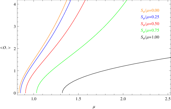
where $c_{1}$ is an integration constant. Obviously, the second term is divergent at the tip $z=1$ if $c_{1}\neq 0$. Considering the Neumann-like boundary condition (6) for the gauge field $A_{t}$ at the tip $z=1$, we have to set $c_{1}=0$ to keep $A_{t}$ finite, i.e., in this case $A_{t}$ will be a constant. Thus, we can get the physical solution $A_{t}(z)=\mu$ to Eq. (13) if $\mu<\mu_{c}$. This is consistent with the numerical results in Figs. 1 and 2 which plot the condensates of the operator $\langle O_{i}\rangle=\psi_{i}$ and charge density $\rho$ with respect to the chemical potential $\mu$ for different values of the dimensionless parameter $k=S_{\varphi}/\mu$.

Similarly, from Eq. (12) we have

which results in a solution

which is consistent with the boundary condition $A_{\varphi}(1)=0$ given in (6).

As $\mu\rightarrow\mu_{c}$ from below the critical point, the scalar field equation (10) becomes

With the boundary condition (7), we assume $\psi$ takes the form

where the trial function $F(z)$ obeys the boundary conditions $F(0)=1$ and $F^{\prime}(0)=0$. From Eq. (17), we arrive at

where we have defined

According to the Sturm-Liouville eigenvalue problem [45], the minimum eigenvalue of $\Lambda=q\mu/r_{s}$ can be obtained from variation of the following functional

where we will assume the trial function to be $F(z)=1-az^{2}$ with a constant $a$. When $k=0$, Eq. (21) reduces to the case considered in [28] for the holographic s-wave insulator/superconductor phase transition, where the spatial component $A_{\varphi}$ has been turned off.

For different values of $k$ and $m^{2}$ with the fixed operator $\langle O_{+}\rangle$ or $\langle O_{-}\rangle$, we can obtain the minimum eigenvalue of $\Lambda^{2}$ and the corresponding value of $a$. As an example, we have $\Lambda_{min}^{2}=3.650$ and $a=0.3214$ for $k=0.25$ with $m^{2}=-15/4$, which gives the critical chemical potential $\Lambda_{c}=\Lambda_{min}=1.911$ for the operator $\langle O_{+}\rangle$. In Table 1, we present the critical chemical potential $\Lambda_{c}=q\mu_{c}/r_{s}$ for chosen $k$ with fixed mass of the scalar field by $m^{2}=-15/4$ in the holographic s-wave superfluid model. Obviously, the agreement of the analytical results derived from the S-L method with the numerical calculation shown in Table 1 is impressive.

We see that, from Table 1 and Figs. 1 and 2, the critical chemical potential $\Lambda_{c}=q\mu_{c}/r_{s}$ increases as the dimensionless parameter $k=S_{\varphi}/\mu$ increases for the fixed mass of the scalar field, i.e., the critical chemical potential becomes larger with the increase of the superfluid velocity, which indicates that the spatial component of the gauge field to modeling the superfluid hinders the phase transition. This result is consistent with the observation obtained from the effective mass of the scalar field in Eq. (5), which implies that the increasing $A_{\varphi}$ will hinder the s-wave superfluid phase transition.

Now we are in a position to study the critical phenomena of this holographic s-wave superfluid system. Considering that the condensation of the scalar operator $\langle O_{i}\rangle$ is so small near the critical point, we can expand $A_{t}(z)$ in $\langle O_{i}\rangle$ as

where we have introduced the boundary condition $\chi(1)=0$ at the tip. Defining a function $\xi(z)$ as

we obtain the equation of motion for $\xi(z)$

with

According to the asymptotic behavior in Eq. (7) and Eq. (23), we will expand $A_{t}$ when $z\rightarrow 0$ as

From the coefficients of the $z^{0}$ term in both sides of the above formula, we have

with

where $c_{2}$ and $c_{3}$ are the integration constants which can be determined by the boundary condition of $\chi(z)$. For example, for the case of $k=0.25$ with $m^{2}=-15/4$, we have $\langle O_{+}\rangle\approx 1.776(\mu-\mu_{c})^{1/2}$ when $a=0.3214$ (we have scaled $q=1$ and $r_{s}=1$ for simplicity), which is in good agreement with the numerical result shown in the left panel of Fig. 1. Note that our expression (27) is valid for all cases considered here, so near the critical point, both of the scalar operators $\langle O_{+}\rangle$ and $\langle O_{-}\rangle$ satisfy $\langle O_{i}\rangle\sim(\mu-\mu_{c})^{1/2}$. This analytical result shows that the phase transition of the holographic s-wave superfluid model belongs to the second order and the critical exponent of the system takes the mean-field value $1/2$, which can be used to back up the numerical findings as shown in Figs. 1 and 2.

Comparing the coefficients of the $z^{1}$ term in Eq. (26), we observe that $\xi^{\prime}(0)\rightarrow 0$, which agrees well with the following relation by making integration of both sides of Eq. (24)

Considering the coefficients of the $z^{2}$ term in Eq. (26), we get

with a prefactor

which is a function of the parameter $k$ and scalar field mass $m^{2}$. For the case of $k=0.25$ and $m^{2}=-15/4$ with the operator $\langle O_{+}\rangle$, as an example, we can obtain $\rho=1.323\left(\mu-\mu_{c}\right)$ when $a=0.3214$ (we have scaled $q=1$ and $r_{s}=1$ for simplicity), which is consistent with the result given in the right panel of Fig. 1. Obviously, the parameter $k$ and mass of the scalar field $m^{2}$ will not change the linear relation between the charge density and chemical potential near $\mu_{c}$, i.e., $\rho\sim(\mu-\mu_{c})$, which is in good agreement with the numerical results plotted in Figs. 1 and 2.

On the other hand, near the critical point Eq. (12) becomes

Thus, we finally arrive at

which obeys the boundary condition $A_{\varphi}(1)=0$ presented in (6) at the critical point. For example, for the case of $k=0.25$ with $m^{2}=-15/4$, we obtain $A_{\varphi}=S_{\varphi}[(1-z^{2})-0.07382\langle O_{+}\rangle^{2}z^{2}+\cdot\cdot\cdot$] when $a=0.3214$ (we have scaled $q=1$ and $r_{s}=1$ for simplicity) for the operator $\langle O_{+}\rangle$. Obviously, Eq. (33) is consistent with the behavior of $A_{\varphi}$ in Eq. (16) at the critical point.

Similar to the analysis for the holographic s-wave model of superfluidity, if $\mu\leq\mu_{c}$, the vector field $\rho_{x}$ is nearly zero, i.e., $\rho_{x}\simeq 0$. Thus, we can obtain the physical solutions $A_{t}(z)=\mu$ to Eq. (42) and $A_{\varphi}=S_{\varphi}(1-z^{2})$ to Eq. (43) when $\mu<\mu_{c}$, which are the same forms just as in the holographic s-wave superfluid model. This analytical result is consistent with the numerical findings in Fig. 3 which plots the condensate of the operator $\langle O_{x}\rangle=\rho_{x+}$ and charge density $\rho$ with respect to the chemical potential $\mu$ for different values of the dimensionless parameter $k=S_{\varphi}/\mu$.

As $\mu\rightarrow\mu_{c}$, the vector field equation (41) will become

Defining a trial function $F(z)$ which matches the boundary behavior (38) for $\rho_{x}$ [26]

with the boundary conditions $F(0)=1$ and $F^{\prime}(0)=0$, from Eq. (44) we can get the equation of motion for $F(z)$

with

where $V(z)$ and $W(z)$ have been introduced in (20). Following the S-L eigenvalue problem [45], we deduce the eigenvalue $\Lambda=q\mu/r_{s}$ minimizes the expression

where we still assume the trial function to be $F(z)=1-az^{2}$ with a constant $a$. When the dimensionless parameter $k=0$, Eq. (48) reduces to the case considered in [37] for the holographic p-wave insulator/superconductor phase transition, where the spatial component $A_{\varphi}$ has been turned off.

For different values of $k$ and $m^{2}$, we can get the minimum eigenvalue of $\Lambda^{2}$ and the corresponding value of $a$, for example, $\Lambda_{min}^{2}=7.879$ and $a=0.3716$ for $k=0.25$ with $m^{2}=5/4$, which leads to the critical chemical potential $\Lambda_{c}=\Lambda_{min}=2.807$. In Table 2, we present the critical chemical potential $\Lambda_{c}=q\mu_{c}/r_{s}$ for chosen $k$. In order to compare with numerical results given in Fig. 3, we fix the mass of the vector field by $m^{2}=5/4$. Obviously, the analytical results derived from S-L method are in very good agreement with the numerical computations.

From Table 2, we observe that, for the fixed mass of the vector field, the critical chemical potential $\Lambda_{c}=q\mu_{c}/r_{s}$ becomes larger with the increase of $k=S_{\varphi}/\mu$, i.e., the critical chemical potential increases with the increase of the superfluid velocity. The fact implies that the spatial component of the gauge field to modeling the superfluid hinders the phase transition, which supports the observation obtained from the effective mass of the vector field in Eq. (36).

Since the condensation of the vector operator $\langle O_{x}\rangle$ is so small when $\mu\rightarrow\mu_{c}$, we can expand $A_{t}(z)$ in small $\langle O_{x}\rangle$ as

with the boundary condition $\chi(1)=0$ at the tip. Introducing a function $\xi(z)$ as

we get the equation of motion for $\xi(z)$

where $Q(z)$ has been defined in (25).

Considering the asymptotic behavior of $A_{t}$ and Eq. (50), near $z\rightarrow 0$ we will expand $A_{t}$ as

According to the coefficients of the $z^{0}$ term in both sides of the above formula, we obtain

with

where $c_{2}$ and $c_{3}$ are the integration constants which can be determined by the boundary condition of $\chi(z)$. For example, for the case of $k=0.25$ with $m^{2}=5/4$, we have $\langle O_{x}\rangle\approx 1.818(\mu-\mu_{c})^{1/2}$ when $a=0.3716$ (we have scaled $q=1$ and $r_{s}=1$ for simplicity), which agrees well with the numerical result shown in the left panel of Fig. 3. Obviously, the expression (53) is valid for all cases considered here. Since the parameter $k$ and mass of the vector field $m^{2}$ will not alter Eq. (53) except for the prefactor, we can obtain the relation $\langle O_{x}\rangle\sim\left(\mu-\mu_{c}\right)^{1/2}$ near the critical point, which shows that the phase transition of the holographic p-wave superfluid model belongs to the second order and the critical exponent of the system takes the mean-field value $1/2$. The analytic result supports the numerical findings obtained from the left panel of Fig. 3.

From the coefficients of the $z^{1}$ term in Eq. (52), we find that $\xi^{\prime}(0)\rightarrow 0$, which is consistent with the following relation by making integration of both sides of Eq. (51)

Comparing the coefficients of the $z^{2}$ term in Eq. (52), we arrive at

with

which is a function of the parameter $k$ and vector field mass $m^{2}$. For the case of $k=0.25$ with $m^{2}=5/4$, as an example, we can obtain $\rho=1.013\left(\mu-\mu_{c}\right)$ when $a=0.3716$ (we have scaled $q=1$ and $r_{s}=1$ for simplicity), which is in good agreement with the result shown in the right panel of Fig. 3. Note that the parameter $k$ and mass of the vector field $m^{2}$ will not alter Eq. (56), we can obtain the linear relation between the charge density and chemical potential near $\mu_{c}$, i.e., $\rho\sim(\mu-\mu_{c})$, which can be used to back up the numerical result presented in the right panel of Fig. 3.

Similarly, considering Eq. (43) near the phase transition point, i.e.,

we can solve it and get

which is consistent with the boundary condition $A_{\varphi}(1)=0$ at the critical point. For example, for the case of $k=0.25$ with $m^{2}=5/4$, we have $A_{\varphi}=S_{\varphi}[(1-z^{2})-0.02450\langle O_{x}\rangle^{2}z^{2}+\cdot\cdot\cdot$] when $a=0.3716$ (we have scaled $q=1$ and $r_{s}=1$ for simplicity), which supports our numerical computation.