The phase-space structure of nearby dark matter as constrained by the SDSS

The fundamental object studied in this paper is the displacement field $\Psi(\textbf{q})$, which maps the initial (Lagrangian) position of particles q to their final (Eulerian) position $\textbf{x}(\textbf{q})$ (see e.g. Bernardeau et al., 2002, for a classic review):

As any smooth vector field, it is possible to split $\Psi$ into a scalar and a rotational part (Chan, 2014, the Helmholtz decomposition,),

where $\Phi_{\Psi}$ is the scalar potential and $\textbf{A}_{\Psi}$ is the vector potential, which obey the Poisson equations:

From analytic approaches and numerical simulations, it has been known for some time that the displacement field is almost fully potential; in particular, $\psi$ contains all the information up to second order in Lagrangian perturbation theory (2LPT). In this paper, we estimate $\psi(\textbf{q})$ and $\textbf{w}(\textbf{q})$ by computing respectively $\mathcal{F}^{-1}[-\mathrm{i}\textbf{k}\cdot\mathcal{F}[\Psi]]$ and $\mathcal{F}^{-1}[\mathrm{i}\textbf{k}\times\mathcal{F}[\Psi]]$, where $\mathcal{F}$ is a fast Fourier transform (FFT) on the Lagrangian mesh on which the displacement field is defined. For later use, we define $\Upsilon(\textbf{q})\equiv\lVert\nabla_{\textbf{q}}~\times~\textbf{A}_{\Psi}\rVert$.

We denote by $J(\textbf{q})$ the Jacobian determinant of the transformation between Lagrangian and Eulerian coordinates,

where the deformation tensor $\mathscr{D}_{\ell m}$ can be written as the identity tensor $\mathscr{I}_{\ell m}\equiv\updelta_{\mathrm{K}}^{\ell,m}$ plus the shear of the displacement field $\mathscr{R}_{\ell m}\equiv\partial\Psi_{\ell}/\partial\textbf{q}_{m}$. The characteristic polynomial of $\mathscr{R}$ is written as

where the $\lambda_{i}$ are the three eigenvalues (real or complex) of $\mathscr{R}$ (i.e. the solutions of $\mathcal{P}_{\mathscr{R}}(\lambda)=0$). The Jacobian is then $J(\textbf{q})=(1+\lambda_{1}(\textbf{q}))(1+\lambda_{2}(\textbf{q}))(1+\lambda_{3}(\textbf{q}))$.

The characteristic equation $\det(\mathscr{R}-\lambda\mathscr{I})=0$ can be written

where we call the $s_{i}$ the Lagrangian invariants (in analogy to the rotational invariants introduced by Wang et al., 2014, who use the shear of the Eulerian velocity field instead of the Lagrangian displacement field). They are given in terms of the eigenvalues by (Chong, Perry & Cantwell, 1990)

from which one can derive the explicit formulation in terms of the coefficients of $\mathscr{R}$ (summation over repeated indices is implied):

In the previous equations, we have used the decomposition of $\mathscr{R}$ into a symmetric part $\uptheta=\left[\theta_{\ell m}\right]$ (the rate of deformation tensor) and an anti-symmetric part $\upomega=\left[\omega_{\ell m}\right]$ (the spin tensor),

with

Physically, $\theta_{\ell m}$ denotes the rate of deformation of a Lagrangian fluid element and $\omega_{\ell m}$ the rate of rotation.

The surface in Lagrangian invariants space that divides real and complex solutions for $\lambda_{i}$ is given by the equation

Using the discriminant of this quadratic equation, one finds two real solutions $s_{3a}$ and $s_{3b}$ ($s_{3a}\leq s_{3b}$) if and only if $s_{2}\leq s_{1}^{2}/3$. Therefore, at fixed $s_{1}$, the regions where all the eigenvalues of $\mathscr{R}$ are real correspond to

In this case, the displacement field is purely potential and we denote the eigenvalues by $\lambda_{1}(\textbf{q})\leq\lambda_{2}(\textbf{q})\leq\lambda_{3}(\textbf{q})$. We also define the ellipticity $\varepsilon$ and prolateness $p$ (Peacock & Heavens, 1985; Bardeen et al., 1986, e.g.) as

Ellipsoids are prolate-like if $-\varepsilon\leq p\leq 0$ or oblate-like if $0\leq p\leq\varepsilon$. The limiting cases are $p=-\varepsilon$ for prolate spheroids and $p=\varepsilon$ for oblate spheroids. In the following, we will also consider $\varepsilon^{\prime}(\textbf{q})\equiv\lambda_{3}(\textbf{q})-\lambda_{1}(\textbf{q})$ and $p^{\prime}(\textbf{q})~\equiv~\lambda_{3}(\textbf{q})-2\lambda_{2}(\textbf{q})+\lambda_{1}(\textbf{q})$, for which the boundary conditions are still valid.

After orbit-crossing, an anti-symmetric part of $\Psi$ is generated and the eigenvalues of $\mathscr{R}$ are no longer all real. We parametrize them as $\lambda_{1,2}(\textbf{q})=a(\textbf{q})\pm\mathrm{i}\,b(\textbf{q})$ and $\lambda_{3}(\textbf{q})=c(\textbf{q})$ where $a,b,c$ are real. The invariants then simply read (see equations (8)–(10))

As we will show in section II.2, the Lagrangian invariants allow a complete classification of the cosmic web, including both potential and vortical flow patterns (Chong, Perry & Cantwell, 1990; Wang et al., 2014, as with the rotational invariants, see).

Finally, we note that it is possible to translate the Lagrangian invariants $s_{i}$ to the eigenvalues $\lambda_{i}$, using Vieta’s formulas for cubic equations:

and for $k\in\{0,1,2\}$,

In our earlier analysis of the volume covered by the SDSS main sample galaxies (60), we adopted the Eulerian cosmic web classifier known as the T-web (Hahn et al., 2007; Forero-Romero et al., 2009). In this framework, structures are classified according to the sign of the eigenvalues $\mu_{1}(\textbf{x})\leq\mu_{2}(\textbf{x})\leq\mu_{3}(\textbf{x})$ of the tidal field tensor $\mathscr{T}$, defined as the Hessian of the rescaled gravitational potential $\Phi$:

where $\Phi$ obeys the reduced Poisson equation

$\delta$ being the local density contrast. A void point corresponds to no positive eigenvalue, a sheet to one, a filament to two, and a cluster to three positive eigenvalues.

Related Hessian-based techniques are the V-web (Hoffman et al., 2012) and classic (Kitaura & Angulo, 2012). More broadly, Eulerian cosmic web algorithms include topological (Aragón-Calvo et al., 2010; Sousbie, 2011), stochastic (González & Padilla, 2010; Tempel et al., 2014), and multiscale field (Aragón-Calvo et al., 2007; Cautun, van de Weygaert & Jones, 2013; Aragon-Calvo & Yang, 2014) methods, all of which yield different physical insights from the phase-space analysis subject of this paper.

In this section, we discuss three alternative methods that can be used for producing Lagrangian classifications of the cosmic web: diva, lich and origami.

Abel, Hahn & Kaehler (2012) and Shandarin, Habib & Heitmann (2012) proposed new techniques to trace the dark matter phase-space sheet and demonstrated that they give a wealth of information previously unavailable in simulations. In this paper, we will demonstrate that these techniques can now be used in data-constrained realizations of the nearby Universe. The core idea is to use a tessellation of the uniform Lagrangian lattice of particles. Each fundamental cube is decomposed into tetrahedral cells that use the particles as their vertices. These cells are tracked in the final conditions, using the particle IDs which are set-up so that they encode the initial position of the particle.

Several possible decompositions of the unit cube exist: for example, Shandarin, Habib & Heitmann (2012) use five tetrahedra of two different volumes. In this work, however, we will follow Abel, Hahn & Kaehler (2012); Hahn, Angulo & Abel (2015) and use the Delaunay decomposition into six identical tetrahedra (see figure 2). Specifically, the connectivity list is $[0,1,3,4]$, $[1,3,4,7]$, $[1,4,5,7]$, $[1,2,5,7]$, $[1,2,3,7]$ and $[2,5,6,7]$ where the unit cube vertices are labeled as in figure 2.

Initially, the volume of each tetrahedron is $d^{3}/6$ where $d$ is the side length of the fundamental cube. In the final state, the same tetrahedron has a volume given by a determinant (or cross-product)

where A, B, C, D label the final positions of the tetrahedron vertices. Note that the volume can be negative if the tetrahedron has been turned inside-out. In fact, the number of sign reversals of an elementary Lagrangian volume defines the flip-flop field (Neyrinck, 2012; Shandarin & Medvedev, 2016, e.g.). Each tetrahedron carries 1/6 of the mass of a particle $m_{\mathrm{p}}$, the mass density associated is therefore $\rho_{\mathrm{tet}}=m_{\mathrm{p}}/\!\left(6|V_{\mathrm{tet}}|\right)$. At any particle position, there are 24 tetrahedra that share this vertex ($2\times 4+4\times 4$, see figure 2).

Tessellating the dark matter phase-space sheet allows one to define a new quantity on the Lagrangian grid, the primordial stream density,

where the summation runs on the 24 tetrahedra that share the particle’s initial position q as one of their vertices. Altogether, these tetrahedra have an initial volume of $24\times d^{3}/6=4\,d^{3}$.

In addition to the primordial stream density, tracking the final configuration of the tessellated dark matter phase-space sheet allows one to perform the Lagrangian transport of any quantity defined on a particle basis, which can be used to define a variety of estimators on the Eulerian grid. This is achieved by finding all the tetrahedra that contain the point x at which properties are to be determined. Each such tetrahedron is given four coefficients $f_{\mathrm{A}}$, $f_{\mathrm{B}}$, $f_{\mathrm{C}}$, $f_{\mathrm{D}}$ for the four particles that constitute its vertices (A, B, C, D). Fields are interpolated inside each tetrahedron using Shepard’s method (inverse distance-squared weighting); namely, each tetrahedron deposits to the point x the quantity

where $w_{\mathrm{P}}\equiv 1/||\textbf{x}-\textbf{x}_{\mathrm{P}}||^{2}$ and $w\equiv\sum_{\mathrm{P}}w_{\mathrm{P}}$.

In this work, we consider the following coefficients and associated estimators:

• •

  $f_{\mathrm{A}}=f_{\mathrm{B}}=f_{\mathrm{C}}=f_{\mathrm{D}}=1$ simply yields the number of tetrahedra enclosing point x. Since we start from a complete tessellation of the considered volume, this is also the number of matter streams contributing at point x, which we call the Eulerian secondary stream density, following Abel, Hahn & Kaehler (2012).

• •

  $f_{\mathrm{A}}=f_{\mathrm{B}}=f_{\mathrm{C}}=f_{\mathrm{D}}=\rho_{\mathrm{tet}}$ yields an estimator of the final Eulerian density field (Abel, Hahn & Kaehler, 2012, see), which we note $\widehat{\rho}_{\mathrm{tet}}$.

• •

  $f_{\mathrm{P}}=\rho_{\mathrm{tet}}$ if particle P is of type $\mathrm{T}_{i}$, 0 otherwise yields an estimator of the density contained in structure of type $\mathrm{T}_{i}$, i.e. $\widehat{\rho}_{\mathrm{tet}}(\mathrm{T}=\mathrm{T}_{i})$. The field $\widehat{\rho}_{\mathrm{tet}}(\mathrm{T}=\mathrm{T}_{i})/\widehat{\rho}_{\mathrm{tet}}$ represents the probability for a final Eulerian point to belong to structure type $\mathrm{T}_{i}$. This method can therefore be used to translate Lagrangian classifications into Eulerian coordinates. As it is computationally expensive, we will introduce a simplified alternative in section IV.2.

• •

  $f_{\mathrm{P}}=v_{s}(\mathrm{P})\times\rho_{\mathrm{tet}}$ where $v_{s}(\mathrm{P})$ is the velocity of particle P along the direction $s\in\{x,y,z\}$ yields an estimator of the component $s$ of the mass-weighted velocity field. The resulting field divided by $\widehat{\rho}_{\mathrm{tet}}$ yields the velocity field estimated from the dark matter phase-space sheet (Hahn, Angulo & Abel, 2015, see).

Instead of explicitly projecting all the tetrahedra to the Eulerian grid, it is possible to approximate each of them by four pseudo-particles (in red in figure 2; see the discussion in Hahn, Abel & Kaehler, 2013, section 2.4, for where to place these pseudo-particles). In this context, the original particles are called the flow tracers and the pseudo-particles are called the mass tracers. Flow tracers uniquely determine the position of mass tracers, which can be deposited to the Eulerian grid by standard interpolation techniques such as the cloud-in-cell (Hockney & Eastwood, 1981, CiC,) algorithm.

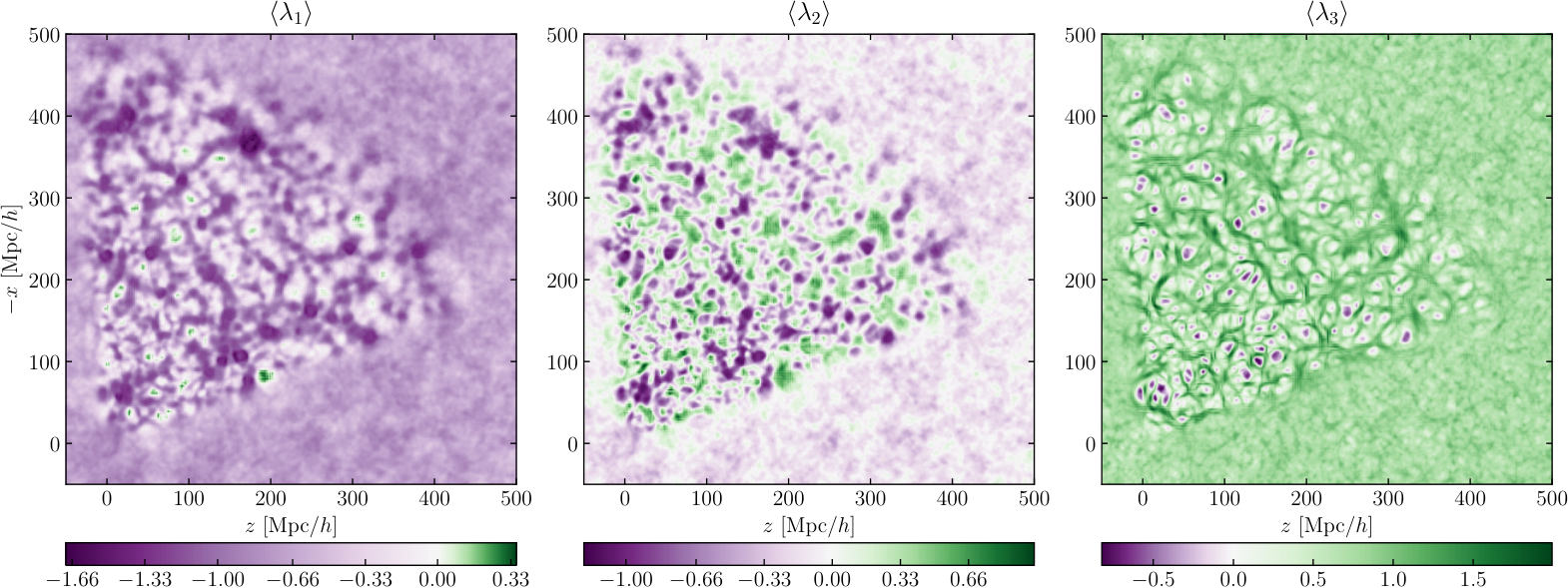
As in our previous work (Jasche, Leclercq & Wandelt, 2015; Leclercq, Jasche & Wandelt, 2015b; Lavaux & Jasche, 2016), the variation among constrained samples constitutes a Bayesian quantification of uncertainties (coming in particular from the survey mask and selection effects). This is illustrated in figure 4, where we show the particle-wise posterior mean of different quantities on the Lagrangian grid. The first row shows the eigenvalues $\lambda_{1}(\textbf{q})\leq\lambda_{2}(\textbf{q})\leq\lambda_{3}(\textbf{q})$ of the rate of deformation tensor $\uptheta$ (the symmetric part of the shear of the displacement field $\mathscr{R}$). These are used by diva to classify structures. The second row shows derived quantities: the (reduced) ellipticity $\varepsilon^{\prime}(\textbf{q})\equiv\lambda_{3}(\textbf{q})-\lambda_{1}(\textbf{q})$ and prolateness $p^{\prime}(\textbf{q})\equiv\lambda_{3}(\textbf{q})-2\lambda_{2}(\textbf{q})+\lambda_{1}(\textbf{q})$, and the Jacobian of the transformation from Lagrangian to Eulerian coordinates, $J(\textbf{q})=(1+\lambda_{1}(\textbf{q}))(1+\lambda_{2}(\textbf{q}))(1+\lambda_{3}(\textbf{q}))$. For each particle, it is the volume of the associated fluid element times its parity (Neyrinck, 2012; Shandarin & Medvedev, 2016). White/blue particles have the same parity as in the initial conditions, while black/orange particles have swapped parity. Caustics are clearly visible wherever blue and orange regions are juxtaposed, for example in the patches that collapse to form halos and in the shell-crossed walls surrounding voids. In some clusters, several parity inversions can be observed. The last row shows the posterior mean for the Lagrangian invariants $s_{1}(\textbf{q})$, $s_{2}(\textbf{q})$, $s_{3}(\textbf{q})$, which are used by lich to classify structures. These cosmographic results constitute the first characterization of the nearby Lagrangian dark matter sheet, and contain a wealth of information on the dynamic large-scale environment of SDSS main sample galaxies. They come as fully probabilistic, which means that uncertainties are quantified at the level of the map.

Uncertainty quantification can also be self-consistently propagated to Lagrangian structure type classification, as we now show. Let us denote by $\xi$ one of the Lagrangian classifiers (diva, lich, or origami). In a specific realization, $\xi$ uniquely characterizes the Lagrangian grid, meaning that it provides $N_{\mathrm{T}}$ particle-wise scalar fields that obey the following conditions for each particle $\textbf{q}_{\ell}$:

where $N_{\mathrm{T}}=4$ for diva and origami ($\mathrm{T}_{0}=$ void, $\mathrm{T}_{1}=$ sheet, $\mathrm{T}_{2}=$ filament, $\mathrm{T}_{3}=$ cluster); $N_{\mathrm{T}}=8$ for lich ($\mathrm{T}_{0}=$ potential void, $\mathrm{T}_{1}=$ potential sheet, $\mathrm{T}_{2}=$ potential filament, $\mathrm{T}_{3}=$ potential cluster, $\mathrm{T}_{4}=$ vortical void, $\mathrm{T}_{5}=$ vortical sheet, $\mathrm{T}_{6}=$ vortical filament, $\mathrm{T}_{7}=$ vortical cluster). By applying $\xi$ to the complete set of borg-cola realizations, we can quantify the degree of belief in structure type classification in terms of $N_{\mathrm{T}}$ particle-wise scalar fields that obey the following conditions for each particle $\textbf{q}_{\ell}$:

Here, $\mathcal{T}_{i}(\textbf{q}_{\ell}|\xi)\equiv\left\langle\mathrm{T}_{i}(\textbf{q}_{\ell}|\xi)\right\rangle_{\mathpzc{P}(\mathrm{T}_{i}(\textbf{q}_{\ell})|d,\xi)}=\mathpzc{P}(\mathrm{T}_{i}(\textbf{q}_{\ell})|d,\xi)$ are the posterior probability distribution functions (pdfs) for particle $\textbf{q}_{\ell}$ to belong to structure $\mathrm{T}_{i}$, as defined by classifier $\xi$, conditional on the data $d$. These are estimated by counting the relative frequencies at each individual particle position within the set of $\xi$-realizations (see also Jasche et al., 2010; 60). Therefore, the cosmic web-type pdf mean on the Lagrangian grid is given by

where $n$ labels one of the $N$ samples, $\mathrm{T}^{n}_{j}(\textbf{q}_{\ell}|\xi)$ is the result of classifier $\xi$ on the $n$-th sample at particle position $\textbf{q}_{\ell}$ (i.e. a unit $N_{\mathrm{T}}$-vector containing zeros except for one component, which indicates the structure type), and $\updelta_{\mathrm{K}}$ is a Kronecker symbol.

Using the above definitions, we obtain probabilistic maps of structures on the Lagrangian grid describing the early Universe in the volume probed by SDSS main sample galaxies. More precisely, for each classifier $\xi$, we obtain a probability mass function (pmf) at each particle position on the Lagrangian grid, indicating the possibility to encounter a specific structure type at that position. These pmfs consist of $N_{\mathrm{T}}$ numbers in the range $[0,1]$, $\mathpzc{P}(\mathrm{T}_{i}(\textbf{q}_{\ell})|d,\xi)$, that sum up to one for each particle. They are approximated by the mean of each structure pdf (see equation (40)).

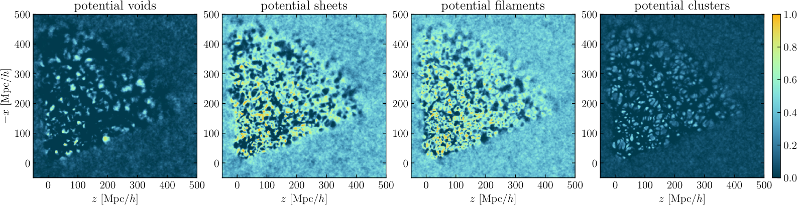
In figure 5, we show slices through these web-type posterior probabilities. The rows represent the structures inferred using diva, lich, and origami, respectively. For comparison, the reader is referred to figure 6 in 60, which shows structures inferred in the initial density field using the T-web. Note that the present results are defined on the Lagrangian grid of $512^{3}$ particles, whereas the T-web result is defined on the $256^{3}$-voxel grid on which initial density fields are discretized. The plot shows the anticipated behavior, with values close to certainty (i.e. zero or one) in regions covered by data, while the unobserved regions (at high redshift or out of the survey boundary) approach a uniform value corresponding to the prior. It is worth noting that different classifiers can have very different prior probabilities for the same structure types (Leclercq et al., 2016, these are given in table II in). The good agreement between diva and lich at the level of individual samples, coming from the absence of a substantial vector part in $\Psi$, is also correctly propagated to the posterior mean.

A voxel-wise quantification of the information gain due to SDSS galaxies is provided by the relative entropy of corresponding posteriors and priors (60; Leclercq et al., 2016). We applied this technique and found that the Lagrangian web-type posteriors presented in figure 5 yield much higher information gain than the application of the T-web to initial density fields. Averaged over the constrained volume, this number is $\sim 0.404$ Sh for diva, $\sim 0.297$ Sh for lich, and $\sim 0.462$ Sh for origami, as compared to $\sim 0.196$ Sh for the T-web. This consideration substantiates the non-local transport of information along Lagrangian trajectories operated by the structure formation model, and demonstrates that a probabilistic description of the Lagrangian dark matter sheet yields a much higher information content for structure type classification than previous methods.

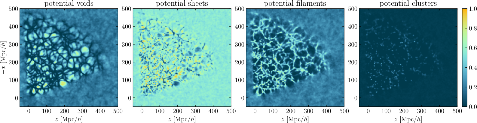
In section III.1.2, we have considered classifications of the dark matter sheet, discretized by the simulation particles. In order to classify structures at redshift zero, it is possible to translate the results of Lagrangian classifiers into Eulerian coordinates. As mentioned in section II.3, a natural way to do this is to use the tessellation of the Lagrangian lattice into tetrahedra, which allows the translation of any particle-wise quantity to the Eulerian grid. However, since this is rather computationally expensive, we introduce below a simplified procedure to translate Lagrangian classifications into Eulerian coordinates. The latter is less precise at the level of individual samples, but we have checked that it yields negligible differences with the respect to the tessellation approach, as far as the posterior mean (figure 8) is concerned.

The simplified approach to translate Lagrangian classifications into Eulerian coordinates works as follows. We consider particles at their final positions and assign them to the Eulerian grid (of $256^{3}$ voxels in our case) using the CiC scheme. For structure type $\mathrm{T}_{i}$, each particle gets a weight of $1$ if its Lagrangian classification is $\mathrm{T}_{i}$, and 0 otherwise. In each voxel, we then count the relative frequencies for each mass-weighted structure type. In this fashion, in each realization $n$, we obtain $N_{\mathrm{T}}$ probabilities, in the range $[0,1]$, for a final Eulerian voxel to belong to each of the structure types. We denote them by $\mathpzc{P}_{n}(\mathrm{T}_{i}(\textbf{x}_{k})|d,\xi)$. In general, we have $\mathcal{S}_{n}(\textbf{x}_{k})\equiv\sum_{i=0}^{N_{\mathrm{T}}-1}\mathpzc{P}_{n}(\mathrm{T}_{i}(\textbf{x}_{k})|d,\xi)=1$; this sum is $0$ if and only if, in realization $n$, no particle was assigned to the cell $\textbf{x}_{k}$ by the CiC scheme (i.e. it is empty as well as its eight neighbors). These voxels are flagged as noisy and discarded.

It is then possible to go from these per-sample pdfs to a global pdf for the entire analysis, in a similar way as before: we count the relative frequencies of the probabilities at each Eulerian spatial position within the set of samples. With this definition, the web-type posterior mean is given by

where $n$ labels one of the $N$ samples, and the normalization $N_{\textbf{x}_{k}}$ in voxel $\textbf{x}_{k}$ is

In figure 8, we show slices through the redshift-zero web-type posterior mean for the different structures as defined by diva, lich, and origami. As before, the plot demonstrates that we are able to propagate typical observational uncertainty to structure type classification. Consistently with the results of section III.1.1, where we argued for the accuracy of the approximation of $\Psi$ to a potential field, we find only small differences between diva voids, sheets, and filaments, and the corresponding lich potential structures. However, unsurprisingly, lich allows a more physical detection and characterization of clusters, where the potential flow assumption breaks down. At this point, the reader is referred to figure 3 in 60 for our map of the same volume, inferred using the T-web definition. The T-web and diva maps are visually similar, with an overall smoother structure for the voids defined by diva, which are sharply separated by walls. diva and lich also visually excel in highlighting the filamentary structure of the cosmic web. In contrast, with origami, most of the volume is filled by voids and more complex, shell-crossed structures are rarely identified.

Understanding large-scale velocity fields is of central importance for modern cosmology: it is linked to galaxy and large-scale structure formation (Pichon & Bernardeau, 1999), is crucial in modeling redshift-space distortions (Percival & White, 2009) and in measuring the kinetic Sunyaev-Zel’dovich effect (Shao et al., 2011; Lavaux, Afshordi & Hudson, 2013). Unfortunately, determining the continuous velocity field is an intrinsically complicated problem, even in simulations, because (i) it is only sampled at discrete locations, with poor resolution in low-density regions; and (ii) it is multi-valued in regions where multiple streams contribute. Typical observational uncertainties (mask, selection effects, galaxy biases) add an additional layer of complexity. Recently, Hahn, Angulo & Abel (2015) showed that the first issues can be overcome in simulations by using the Lagrangian phase-space sheet. We apply this technique to our set of constrained simulations and demonstrate that we can also circumvent the observational complications. In doing so, we provide unprecedentedly accurate reconstruction of cosmic velocity fields in the volume of the nearby Universe covered by the northern galactic cap of the SDSS main galaxy sample and its surroundings.

We applied the estimators described in section II.3 to our set of constrained simulations, and obtained the components of the velocity field $v_{x}$, $v_{y}$, $v_{z}$, on Eulerian grids of $256^{3}$ and $512^{3}$ voxels. As shown in the beginning of section IV, under the assumption that velocities are conditionally independent of the data once initial conditions are known, these samples are drawn from $\mathpzc{P}(\textbf{v}|d)$. As before, each of them gives one plausible realization of the velocity field, and the variation between samples quantifies the remaining uncertainty. In figure 9, we show the posterior mean for the three spherical components of the velocity field, in the celestial equator. The interested reader may want to compare with figure 7 in 44, which showed the velocity field as probed by 2LPT particles in one particular sample. The present work constitutes a substantial improvement over these results, since the velocity field is now predicted by a fully non-linear structure formation model instead of 2LPT, well-sampled even in low-density regions, and with more straightforward uncertainty quantification. The recovered velocity field is fully compatible with the known structure of the nearby Universe; showing, for example, the infall of matter onto the Sloan Great Wall.

As noted in 44, velocity fields are derived a posteriori with borg, i.e. they are a prediction of physical models given the inferred initial density field.³³ 3 In contrast, algorithms like virbius (Lavaux, 2016) explicitly exploit velocity information contained in the data to constrain the result, and reconstructions based on surveys of peculiar velocities have produced highly appealing results (Courtois et al., 2013; Tully et al., 2014, e.g.). However, since velocity fields are predominantly governed by large-scale modes, which are accurately recovered by borg (44), any improvement in the inference scheme is not expected to crucially change our results.

To characterize the accuracy at which our velocity fields are predicted, we analyzed their spectral properties against that of reference simulations produced with the same setup (60, presented in). From the Cartesian velocity components,⁴⁴ 4 We do not use the divergence and curl directly computed using Lagrangian transport, but rather from the velocity field itself, for the reasons discussed in Hahn, Angulo & Abel (2015, section 5.1). we computed the divergence and the curl,

using FFTs on the Eulerian grid of side length 750 Mpc/$h$ and $256^{3}$ voxels. We computed their respective power spectra, given by

To test the proportionality between $\theta$ and the density contrast $\delta$, valid at first order in Lagrangian perturbation theory, we also computed the cross- and auto-power spectra

In this case, $\delta$ is estimated by standard CiC deposit of dark matter particles to the grid, and we apply a correction factor for aliasing effects and suppression of small-scale power close to the Nyquist wavenumber (Jing, 2005).⁵⁵ 5 We here rely on the CiC scheme and not on the phase-space density fields estimators, following the arguments of Hahn, Angulo & Abel (2015, section 5.2).

In figure 10, we show $P_{\theta\theta}$, $P_{\omega\omega}$, $P_{\theta\omega}$ and $P_{\delta\delta}$ as a function of the wavenumber $k$. The measurements from our simulations agree with the results of Hahn, Angulo & Abel (2015). The plots confirm the agreement between unconstrained and constrained density fields ($\delta\delta$) at all scales (already discussed in 60).⁶⁶ 6 We note that a lack of small scale power with respect to theoretical predictions, for $k\gtrsim 0.5~(\mathrm{Mpc}/h)^{-1}$, is observed in both unconstrained and constrained realizations. This is a gridding artifact due to the finite mesh size used to compute power spectra. This scale corresponds to around one quarter of the Nyquist wavenumber. Remarkable agreement with simulations can also be observed for $\theta\delta$ and $\theta\theta$ correlations. Deviations can only be observed for $k\gtrsim 0.4~(\mathrm{Mpc}/h)^{-1}$. Below this scale, structure formation becomes notably non-linear, meaning that the 2LPT model used in the borg inference process breaks down, which explains the lack of small-scale power when the constrained initial conditions are run forward with a fully non-linear code. The lack of $\theta\delta$ and $\theta\theta$ correlations does not exceed $\sim$ 30% for $k=1~(\mathrm{Mpc}/h)^{-1}$. Since the velocity field is curl-free in 2LPT, the vorticity $\boldsymbol{\omega}$ is a unique prediction of the physical model accounting for full gravity. Strikingly, the prediction for $P_{\omega\omega}$ still agrees well with the result of unconstrained simulations, meaning that cola filtering reinstates most of the final vorticity, and does so consistently with the inferred phases (see the $\Upsilon$ panel in figure 3). Discrepancies are limited to an almost scale-independent negative offset of $\sim$ 35%, which can be explained by known limitations of the borg data model: use of 2LPT instead of fully non-linear gravity, only partial fitting of galaxy bias, absence of redshift-space distortions and lightcone effects.

Summing up this section, at the demonstrated degree of accuracy, our results go beyond the state of the art for the characterization of cosmic velocity fields in the SDSS volume, including its low galaxy-density regions. They include the first quantitative prediction of the vorticity field, and come with the possibility of uncertainty quantification at the level of fields and summary statistics.

For illustration purposes, as well as to demonstrate the power of inferring the phase-space structure of dark matter, we discuss in this section some cosmographic results concerning well-known objects of the Local Universe. We have already discussed the Sloan Great Wall (Gott et al., 2005; Einasto et al., 2011), at celestial equatorial coordinates $220\degree\lesssim\alpha\lesssim 150\degree$, $-4\degree\lesssim\delta\lesssim 8\degree$, $150\lesssim r\lesssim 300$ Mpc/$h$, visible in figures 3, 6 and 9.

In figure 11, we show slices through the supergalactic plane (SGP). The supergalactic coordinate system is defined by the position of its North Pole ($B=90\degree$) in the direction of Galactic coordinates ($l=47.37\degree$; $b=+6.32\degree$, Lahav et al., 2000). The portion of the SGP ($B=0\degree$) which is constrained in our analysis corresponds to $30\lesssim L\lesssim 120\degree$, the rest is not covered by the SDSS main galaxy sample. The different panels show the posterior mean for: the density estimated from mass tracers (see section IV.1.2), the secondary stream density (see section IV.1.1), and the radial velocity field (see section IV.3). Galaxies in a $10$ Mpc/$h$-thick slice are overplotted. Some major structures of the Local Universe are clearly visible: the Coma cluster ($L\sim 90\degree$, $r\sim 70$ Mpc/$h$), the Ursa-Majoris supercluster ($L\sim 60\degree$, $r\sim 170$ Mpc/$h$), and two farther clusters in the direction of Ursa-Major ($L\sim 70\degree$, $r\sim 220$ Mpc/$h$) and Ursa-Major/Coma-Berenices ($L\sim 82\degree$, $r\sim 220$ Mpc/$h$) (Abell, Corwin & Olowin, 1989, e.g.). One can also notice part of Leo supercluster ($L\sim 85\degree$, $r\sim 95$ Mpc/$h$), which is mostly below the SGP (at $B\sim-18\degree$). Three voids intersect the SGP: the well-known Boötes void (Kirshner et al., 1981), whose center is above the SGP ($L\sim 84\degree$, $B\sim 18\degree$, $r\sim 150$ Mpc/$h$) and which is around $200$ Mpc/$h$ in radius (Batuski & Burns, 1985), a void in the direction of Ursa-Major ($L\sim 47\degree$, $r\sim 60$ Mpc/$h$), and one in the direction of Coma-Berenices ($L\sim 104\degree$, $r\sim 50$ Mpc/$h$) (Fairall, 1998, e.g.). Part of the Virgo-Boötes-Hercules (VBH) filament, which extends from $L\sim 100\degree$ to $L\sim 150\degree$ at $r\sim 140$ Mpc/$h$ (Lavaux & Jasche, 2016) is also visible. For comparison, see also figure 4 in Carrick et al. (2015) and figure 7 in Lavaux & Jasche (2016).

As expected, structures observed in galaxies correlate well with the reconstructed dark matter density. At this mass resolution, up to 5 matter streams converge in the inner regions of Coma, the Ursa-Majoris supercluster, and the VBH filament. The voids in Coma-Berenices and in Ursa-Major are single-stream regions, as well as most voids of the Local Universe. However, our analysis reveals some substructure of the Boötes void. Reconstructed velocity fields gives further dynamical insight into these structures. Superclusters are still accreting matter, as seen in radial velocity “dipoles”. The ongoing emptying of voids is also clearly observable; for example, dark matter inside the Boötes void is streaming out towards its surrounding overdensities, the Coma cluster and the VBH filament.

References

- Abel, Hahn & Kaehler (2012) (Abel, Hahn & Kaehler, 2012) T. Abel, O. Hahn, R. Kaehler, Tracing the dark matter sheet in phase space, Mon. Not. R. Astron. Soc. 427, 61 (2012), arXiv:1111.3944 [astro-ph.CO].
- Abell, Corwin & Olowin (1989) (Abell, Corwin & Olowin, 1989) G. O. Abell, H. G. Corwin, Jr., R. P. Olowin, A catalog of rich clusters of galaxies, Astrophys. J. Supp. 70, 1 (1989).
- Aragon-Calvo & Szalay (2013) (Aragon-Calvo & Szalay, 2013) M. A. Aragon-Calvo, A. S. Szalay, The hierarchical structure and dynamics of voids, Mon. Not. R. Astron. Soc. 428, 3409 (2013), arXiv:1203.0248 [astro-ph.CO].
- Aragon-Calvo & Yang (2014) (Aragon-Calvo & Yang, 2014) M. A. Aragon-Calvo, L. F. Yang, The hierarchical nature of the spin alignment of dark matter haloes in filaments, Mon. Not. R. Astron. Soc. 440, L46 (2014), arXiv:1303.1590 [astro-ph.CO].
- Aragón-Calvo et al. (2007) (Aragón-Calvo et al., 2007) M. A. Aragón-Calvo, B. J. T. Jones, R. van de Weygaert, J. M. van der Hulst, The multiscale morphology filter: identifying and extracting spatial patterns in the galaxy distribution, Astron. & Astrophys. 474, 315 (2007), arXiv:0705.2072.
- Aragón-Calvo et al. (2010) (Aragón-Calvo et al., 2010) M. A. Aragón-Calvo, E. Platen, R. van de Weygaert, A. S. Szalay, The Spine of the Cosmic Web, Astrophys. J. 723, 364 (2010), arXiv:0809.5104.
- Arnold, Shandarin & Zeldovich (1982) (Arnold, Shandarin & Zeldovich, 1982) V. I. Arnold, S. F. Shandarin, I. B. Zeldovich, The large scale structure of the universe. I - General properties One- and two-dimensional models, Geophysical and Astrophysical Fluid Dynamics 20, 111 (1982).
- Bardeen et al. (1986) (Bardeen et al., 1986) J. M. Bardeen, J. R. Bond, N. Kaiser, A. S. Szalay, The statistics of peaks of Gaussian random fields, Astrophys. J. 304, 15 (1986).
- Batuski & Burns (1985) (Batuski & Burns, 1985) D. J. Batuski, J. O. Burns, Finding lists of candidate superclusters and voids of Abell clusters, Astronom. J. 90, 1413 (1985).
- Bernardeau et al. (2002) (Bernardeau et al., 2002) F. Bernardeau, S. Colombi, E. Gaztañaga, R. Scoccimarro, Large-scale structure of the Universe and cosmological perturbation theory, Physics Reports 367, 1 (2002), astro-ph/0112551.
- Blanton et al. (2005) (Blanton et al., 2005) M. R. Blanton, D. Eisenstein, D. W. Hogg, D. J. Schlegel, J. Brinkmann, Relationship between Environment and the Broadband Optical Properties of Galaxies in the Sloan Digital Sky Survey, Astrophys. J. 629, 143 (2005), astro-ph/0310453.
- Bond, Kofman & Pogosyan (1996) (Bond, Kofman & Pogosyan, 1996) J. R. Bond, L. Kofman, D. Pogosyan, How filaments of galaxies are woven into the cosmic web, Nature 380, 603 (1996), astro-ph/9512141.
- Burden, Percival & Howlett (2015) (Burden, Percival & Howlett, 2015) A. Burden, W. J. Percival, C. Howlett, Reconstruction in Fourier space, Mon. Not. R. Astron. Soc. 453, 456 (2015), arXiv:1504.02591.
- Carrick et al. (2015) (Carrick et al., 2015) J. Carrick, S. J. Turnbull, G. Lavaux, M. J. Hudson, Cosmological parameters from the comparison of peculiar velocities with predictions from the 2M++ density field, Mon. Not. R. Astron. Soc. 450, 317 (2015), arXiv:1504.04627.
- Cautun, van de Weygaert & Jones (2013) (Cautun, van de Weygaert & Jones, 2013) M. Cautun, R. van de Weygaert, B. J. T. Jones, NEXUS: tracing the cosmic web connection, Mon. Not. R. Astron. Soc. 429, 1286 (2013), arXiv:1209.2043 [astro-ph.CO].
- Cautun et al. (2014) (Cautun et al., 2014) M. Cautun, R. van de Weygaert, B. J. T. Jones, C. S. Frenk, Evolution of the cosmic web, Mon. Not. R. Astron. Soc. 441, 2923 (2014), arXiv:1401.7866.
- Chan (2014) (Chan, 2014) K. C. Chan, Helmholtz decomposition of the Lagrangian displacement, Phys. Rev. D 89, 083515 (2014), arXiv:1309.2243.
- Chong, Perry & Cantwell (1990) (Chong, Perry & Cantwell, 1990) M. S. Chong, A. E. Perry, B. J. Cantwell, A general classification of three-dimensional flow fields, Physics of Fluids 2, 765 (1990).
- Codis et al. (2015) (Codis et al., 2015) S. Codis, R. Gavazzi, Y. Dubois, C. Pichon, K. Benabed, V. Desjacques, D. Pogosyan, J. Devriendt, A. Slyz, Intrinsic alignment of simulated galaxies in the cosmic web: implications for weak lensing surveys, Mon. Not. R. Astron. Soc. 448, 3391 (2015), arXiv:1406.4668.
- Courtois et al. (2013) (Courtois et al., 2013) H. M. Courtois, D. Pomarède, R. B. Tully, Y. Hoffman, D. Courtois, Cosmography of the Local Universe, Astronom. J. 146, 69 (2013), arXiv:1306.0091.
- Davis et al. (2011) (Davis et al., 2011) T. M. Davis, L. Hui, J. A. Frieman, T. Haugbølle, R. Kessler, B. Sinclair, J. Sollerman, B. Bassett, J. Marriner, E. Mörtsell, R. C. Nichol, M. W. Richmond, M. Sako, D. P. Schneider, M. Smith, The Effect of Peculiar Velocities on Supernova Cosmology, Astrophys. J. 741, 67 (2011), arXiv:1012.2912.
- Einasto et al. (2011) (Einasto et al., 2011) M. Einasto, L. J. Liivamägi, E. Tempel, E. Saar, E. Tago, P. Einasto, I. Enkvist, J. Einasto, V. J. Martínez, P. Heinämäki, P. Nurmi, The Sloan Great Wall. Morphology and Galaxy Content, Astrophys. J. 736, 51 (2011), arXiv:1105.1632.
- Eisenstein et al. (2007) (Eisenstein et al., 2007) D. J. Eisenstein, H.-J. Seo, E. Sirko, D. N. Spergel, Improving Cosmological Distance Measurements by Reconstruction of the Baryon Acoustic Peak, Astrophys. J. 664, 675 (2007), astro-ph/0604362.
- Fairall (1998) (Fairall, 1998) A. P. Fairall, Large-scale structures in the universe, Wiley-Praxis series in astronomy and astrophysics (Wiley, 1998).
- Falck, Neyrinck & Szalay (2012) (Falck, Neyrinck & Szalay, 2012) B. L. Falck, M. C. Neyrinck, A. S. Szalay, ORIGAMI: Delineating Halos Using Phase-space Folds, Astrophys. J. 754, 126 (2012), arXiv:1201.2353 [astro-ph.CO].
- Falck & Neyrinck (2015) (Falck & Neyrinck, 2015) B. Falck, M. C. Neyrinck, The persistent percolation of single-stream voids, Mon. Not. R. Astron. Soc. 450, 3239 (2015), arXiv:1410.4751.
- Falck, Koyama & Zhao (2015) (Falck, Koyama & Zhao, 2015) B. Falck, K. Koyama, G.-B. Zhao, Cosmic web and environmental dependence of screening: Vainshtein vs. chameleon, Journal of Cosmology and Astroparticle Physics 7, 049 (2015), arXiv:1503.06673 [astro-ph.CO].
- Feldbrugge, Hidding & van de Weygaert (2014) (Feldbrugge, Hidding & van de Weygaert, 2014) J. Feldbrugge, J. Hidding, R. van de Weygaert, Statistics of Caustics in Large-Scale Structure Formation, in The Zeldovich Universe: Genesis and Growth of the Cosmic Web, Proceedings of IAU Symposium 308, 23-28 June 2014, Tallinn, Estonia, edited by R. van de Weygaert, S. Shandarin, E. Saar, J. Einasto (Cambridge University Press, 2014) pp. 107–114, arXiv:1412.5121.
- Feldbrugge et al. (2017) (Feldbrugge et al., 2017) J. Feldbrugge, R. van de Weygaert, J. Hidding, J. Feldbrugge, Caustic conditions for d-dimensional Lagrangian fluids, ArXiv e-prints (2017), arXiv:1703.09598 [physics.flu-dyn].
- Forero-Romero et al. (2009) (Forero-Romero et al., 2009) J. E. Forero-Romero, Y. Hoffman, S. Gottlöber, A. Klypin, G. Yepes, A dynamical classification of the cosmic web, Mon. Not. R. Astron. Soc. 396, 1815 (2009), arXiv:0809.4135 [astro-ph].
- Gao et al. (2012) (Gao et al., 2012) L. Gao, C. S. Frenk, A. Jenkins, V. Springel, S. D. M. White, Where will supersymmetric dark matter first be seen?, Mon. Not. R. Astron. Soc. 419, 1721 (2012), arXiv:1107.1916 [astro-ph.CO].
- González & Padilla (2010) (González & Padilla, 2010) R. E. González, N. D. Padilla, Automated detection of filaments in the large-scale structure of the Universe, Mon. Not. R. Astron. Soc. 407, 1449 (2010), arXiv:0912.0006 [astro-ph.CO].
- Gott et al. (2005) (Gott et al., 2005) J. R. Gott, III, M. Jurić, D. Schlegel, F. Hoyle, M. Vogeley, M. Tegmark, N. Bahcall, J. Brinkmann, A Map of the Universe, Astrophys. J. 624, 463 (2005), astro-ph/0310571.
- Gurbatov, Saichev & Shandarin (1989) (Gurbatov, Saichev & Shandarin, 1989) S. N. Gurbatov, A. I. Saichev, S. F. Shandarin, The large-scale structure of the universe in the frame of the model equation of non-linear diffusion, Mon. Not. R. Astron. Soc. 236, 385 (1989).
- Gurbatov, Saichev & Shandarin (2012) (Gurbatov, Saichev & Shandarin, 2012) S. N. Gurbatov, A. I. Saichev, S. F. Shandarin, Large-scale structure of the Universe. The Zeldovich approximation and the adhesion model, Physics Uspekhi 55, 223 (2012).
- Hahn, Abel & Kaehler (2013) (Hahn, Abel & Kaehler, 2013) O. Hahn, T. Abel, R. Kaehler, A new approach to simulating collisionless dark matter fluids, Mon. Not. R. Astron. Soc. 434, 1171 (2013), arXiv:1210.6652.
- Hahn, Angulo & Abel (2015) (Hahn, Angulo & Abel, 2015) O. Hahn, R. E. Angulo, T. Abel, The properties of cosmic velocity fields, Mon. Not. R. Astron. Soc. 454, 3920 (2015), arXiv:1404.2280.
- Hahn et al. (2007) (Hahn et al., 2007) O. Hahn, C. Porciani, C. M. Carollo, A. Dekel, Properties of dark matter haloes in clusters, filaments, sheets and voids, Mon. Not. R. Astron. Soc. 375, 489 (2007), astro-ph/0610280.
- Hidding, Shandarin & van de Weygaert (2014) (Hidding, Shandarin & van de Weygaert, 2014) J. Hidding, S. F. Shandarin, R. van de Weygaert, The Zel’dovich approximation: key to understanding cosmic web complexity, Mon. Not. R. Astron. Soc. 437, 3442 (2014), arXiv:1311.7134 [astro-ph.CO].
- Hidding, van de Weygaert & Shandarin (2016) (Hidding, van de Weygaert & Shandarin, 2016) J. Hidding, R. van de Weygaert, S. Shandarin, The Zeldovich & Adhesion approximations and applications to the local universe, in The Zeldovich Universe: Genesis and Growth of the Cosmic Web, Proceedings of IAU Symposium 308, 23-28 June 2014, Tallinn, Estonia, edited by R. van de Weygaert, S. Shandarin, E. Saar, J. Einasto (Cambridge University Press, 2016) pp. 69–76, arXiv:1611.01221.
- Hockney & Eastwood (1981) (Hockney & Eastwood, 1981) R. W. Hockney, J. W. Eastwood, Computer Simulation Using Particles (McGraw-Hill, 1981).
- Hoffman et al. (2012) (Hoffman et al., 2012) Y. Hoffman, O. Metuki, G. Yepes, S. Gottlöber, J. E. Forero-Romero, N. I. Libeskind, A. Knebe, A kinematic classification of the cosmic web, Mon. Not. R. Astron. Soc. 425, 2049 (2012), arXiv:1201.3367 [astro-ph.CO].
- Jasche & Wandelt (2013) (Jasche & Wandelt, 2013) J. Jasche, B. D. Wandelt, Bayesian physical reconstruction of initial conditions from large-scale structure surveys, Mon. Not. R. Astron. Soc. 432, 894 (2013), arXiv:1203.3639 [astro-ph.CO].
- Jasche, Leclercq & Wandelt (2015) (Jasche, Leclercq & Wandelt, 2015) J. Jasche, F. Leclercq, B. D. Wandelt, Past and present cosmic structure in the SDSS DR7 main sample, Journal of Cosmology and Astroparticle Physics 1, 036 (2015), arXiv:1409.6308 [astro-ph.CO].
- Jasche et al. (2010) (Jasche et al., 2010) J. Jasche, F. S. Kitaura, C. Li, T. A. Enßlin, Bayesian non-linear large-scale structure inference of the Sloan Digital Sky Survey Data Release 7, Mon. Not. R. Astron. Soc. 409, 355 (2010), arXiv:0911.2498 [astro-ph.CO].
- Jing (2005) (Jing, 2005) Y. P. Jing, Correcting for the Alias Effect When Measuring the Power Spectrum Using a Fast Fourier Transform, Astrophys. J. 620, 559 (2005), astro-ph/0409240.
- Kirshner et al. (1981) (Kirshner et al., 1981) R. P. Kirshner, A. Oemler, Jr., P. L. Schechter, S. A. Shectman, A million cubic megaparsec void in Bootes, Astrophys. J. Lett. 248, L57 (1981).
- Kitaura & Angulo (2012) (Kitaura & Angulo, 2012) F.-S. Kitaura, R. E. Angulo, Linearization with cosmological perturbation theory, Mon. Not. R. Astron. Soc. 425, 2443 (2012), arXiv:1111.6617.
- Knebe et al. (2011) (Knebe et al., 2011) A. Knebe, S. R. Knollmann, S. I. Muldrew, F. R. Pearce, M. A. Aragon-Calvo, Y. Ascasibar, P. S. Behroozi, D. Ceverino, S. Colombi, J. Diemand, K. Dolag, B. L. Falck, P. Fasel, J. Gardner, S. Gottlöber, C.-H. Hsu, F. Iannuzzi, A. Klypin, Z. Lukić, M. Maciejewski, C. McBride, M. C. Neyrinck, S. Planelles, D. Potter, V. Quilis, Y. Rasera, J. I. Read, P. M. Ricker, F. Roy, V. Springel, J. Stadel, G. Stinson, P. M. Sutter, V. Turchaninov, D. Tweed, G. Yepes, M. Zemp, Haloes gone MAD: The Halo-Finder Comparison Project, Mon. Not. R. Astron. Soc. 415, 2293 (2011), arXiv:1104.0949.
- Kofman, Pogosian & Shandarin (1990) (Kofman, Pogosian & Shandarin, 1990) L. Kofman, D. Pogosian, S. Shandarin, Structure of the universe in the two-dimensional model of adhesion, Mon. Not. R. Astron. Soc. 242, 200 (1990).
- Kofman et al. (1992) (Kofman et al., 1992) L. Kofman, D. Pogosyan, S. F. Shandarin, A. L. Melott, Coherent structures in the universe and the adhesion model, Astrophys. J. 393, 437 (1992).
- Lahav et al. (2000) (Lahav et al., 2000) O. Lahav, B. X. Santiago, A. M. Webster, M. A. Strauss, M. Davis, A. Dressler, J. P. Huchra, The supergalactic plane revisited with the Optical Redshift Survey, Mon. Not. R. Astron. Soc. 312, 166 (2000).
- Larsen & Challinor (2016) (Larsen & Challinor, 2016) P. Larsen, A. Challinor, Intrinsic alignment contamination to CMB lensing-galaxy weak lensing correlations from tidal torquing, Mon. Not. R. Astron. Soc. 461, 4343 (2016), arXiv:1510.02617.
- Lavaux (2016) (Lavaux, 2016) G. Lavaux, Bayesian 3D velocity field reconstruction with VIRBIUS, Mon. Not. R. Astron. Soc. 457, 172 (2016), arXiv:1512.04534.
- Lavaux & Jasche (2016) (Lavaux & Jasche, 2016) G. Lavaux, J. Jasche, Unmasking the masked Universe: the 2M++ catalogue through Bayesian eyes, Mon. Not. R. Astron. Soc. 455, 3169 (2016), arXiv:1509.05040 [astro-ph.CO].
- Lavaux & Wandelt (2010) (Lavaux & Wandelt, 2010) G. Lavaux, B. D. Wandelt, Precision cosmology with voids: definition, methods, dynamics, Mon. Not. R. Astron. Soc. 403, 1392 (2010), arXiv:0906.4101 [astro-ph.CO].
- Lavaux, Afshordi & Hudson (2013) (Lavaux, Afshordi & Hudson, 2013) G. Lavaux, N. Afshordi, M. J. Hudson, First measurement of the bulk flow of nearby galaxies using the cosmic microwave background, Mon. Not. R. Astron. Soc. 430, 1617 (2013), arXiv:1207.1721.
- Leclercq (2015) (Leclercq, 2015) F. Leclercq, Bayesian large-scale structure inference and cosmic web analysis, Ph.D. thesis, Institut d’Astrophysique de Paris (2015), arXiv:1512.04985 [astro-ph.CO].
- Leclercq, Jasche & Wandelt (2015a) (Leclercq, Jasche & Wandelt, 2015a) F. Leclercq, J. Jasche, B. Wandelt, Cosmic web-type classification using decision theory, Astron. & Astrophys. 576, L17 (2015a), arXiv:1503.00730 [astro-ph.CO].
- Leclercq, Jasche & Wandelt (2015b) (Leclercq, Jasche & Wandelt, 2015b) F. Leclercq, J. Jasche, B. Wandelt, Bayesian analysis of the dynamic cosmic web in the SDSS galaxy survey, Journal of Cosmology and Astroparticle Physics 6, 015 (2015b), arXiv:1502.02690 [astro-ph.CO].
- Leclercq et al. (2016) (Leclercq et al., 2016) F. Leclercq, G. Lavaux, J. Jasche, B. Wandelt, Comparing cosmic web classifiers using information theory, Journal of Cosmology and Astroparticle Physics 8, 027 (2016), arXiv:1606.06758 [astro-ph.CO].
- Leclercq et al. (2015) (Leclercq et al., 2015) F. Leclercq, J. Jasche, P. M. Sutter, N. Hamaus, B. Wandelt, Dark matter voids in the SDSS galaxy survey, Journal of Cosmology and Astroparticle Physics 3, 047 (2015), arXiv:1410.0355 [astro-ph.CO].
- Libeskind et al. (2015) (Libeskind et al., 2015) N. I. Libeskind, Y. Hoffman, R. B. Tully, H. M. Courtois, D. Pomarède, S. Gottlöber, M. Steinmetz, Planes of satellite galaxies and the cosmic web, Mon. Not. R. Astron. Soc. 452, 1052 (2015), arXiv:1503.05915.
- Libeskind et al. (2017) (Libeskind et al., 2017) N. I. Libeskind, R. van de Weygaert, M. Cautun, B. Falck, E. Tempel, T. Abel, M. Alpaslan, M. A. Aragoon-Calvo, J. E. Forero-Romero, R. Gonzalez, S. Gottloober, O. Hahn, W. A. Hellwing, Y. Hoffman, B. J. T. Jones, F. Kitaura, A. Knebe, S. Manti, M. Neyrinck, S. E. Nuza, N. Padilla, E. Platen, N. Ramachandra, A. Robotham, E. Saar, S. Shandarin, M. Steinmetz, R. S. Stoica, T. Sousbie, G. Yepes, Tracing the cosmic web, ArXiv e-prints (2017), arXiv:1705.03021.
- Neyrinck (2013) (Neyrinck, 2013) M. C. Neyrinck, Quantifying distortions of the Lagrangian dark-matter mesh in cosmology, Mon. Not. R. Astron. Soc. 428, 141 (2013), arXiv:1204.1326 [astro-ph.CO].
- Neyrinck (2012) (Neyrinck, 2012) M. C. Neyrinck, Origami constraints on the initial-conditions arrangement of dark-matter caustics and streams, Mon. Not. R. Astron. Soc. 427, 494 (2012), arXiv:1202.3364 [astro-ph.CO].
- Padmanabhan et al. (2012) (Padmanabhan et al., 2012) N. Padmanabhan, X. Xu, D. J. Eisenstein, R. Scalzo, A. J. Cuesta, K. T. Mehta, E. Kazin, A 2 per cent distance to z = 0.35 by reconstructing baryon acoustic oscillations - I. Methods and application to the Sloan Digital Sky Survey, Mon. Not. R. Astron. Soc. 427, 2132 (2012), arXiv:1202.0090.
- Peacock & Heavens (1985) (Peacock & Heavens, 1985) J. A. Peacock, A. F. Heavens, The statistics of maxima in primordial density perturbations, Mon. Not. R. Astron. Soc. 217, 805 (1985).
- Percival & White (2009) (Percival & White, 2009) W. J. Percival, M. White, Testing cosmological structure formation using redshift-space distortions, Mon. Not. R. Astron. Soc. 393, 297 (2009), arXiv:0808.0003.
- Pichon & Bernardeau (1999) (Pichon & Bernardeau, 1999) C. Pichon, F. Bernardeau, Vorticity generation in large-scale structure caustics, Astron. & Astrophys. 343, 663 (1999), astro-ph/9902142.
- Planck Collaboration (2014) (Planck Collaboration, 2014) Planck Collaboration, Planck 2013 results. XIX. The integrated Sachs-Wolfe effect, Astron. & Astrophys. 571, A19 (2014), arXiv:1303.5079 [astro-ph.CO].
- Ramachandra & Shandarin (2017) (Ramachandra & Shandarin, 2017) N. S. Ramachandra, S. F. Shandarin, Topology and geometry of the dark matter web: A multi-stream view, Mon. Not. R. Astron. Soc. 467, 1748 (2017), arXiv:1608.05469.
- Ramachandra & Shandarin (2015) (Ramachandra & Shandarin, 2015) N. S. Ramachandra, S. F. Shandarin, Multi-stream portrait of the cosmic web, Mon. Not. R. Astron. Soc. 452, 1643 (2015), arXiv:1412.7768.
- Shandarin & Medvedev (2016) (Shandarin & Medvedev, 2016) S. F. Shandarin, M. V. Medvedev, The features of the Cosmic Web unveiled by the flip-flop field, ArXiv e-prints (2016), arXiv:1609.08554.
- Shandarin, Habib & Heitmann (2012) (Shandarin, Habib & Heitmann, 2012) S. Shandarin, S. Habib, K. Heitmann, Cosmic web, multistream flows, and tessellations, Phys. Rev. D 85, 083005 (2012), arXiv:1111.2366 [astro-ph.CO].
- Shao et al. (2011) (Shao et al., 2011) J. Shao, P. Zhang, W. Lin, Y. Jing, J. Pan, Kinetic Sunyaev-Zel’dovich tomography with spectroscopic redshift surveys, Mon. Not. R. Astron. Soc. 413, 628 (2011), arXiv:1004.1301.
- Sousbie (2011) (Sousbie, 2011) T. Sousbie, The persistent cosmic web and its filamentary structure - I. Theory and implementation, Mon. Not. R. Astron. Soc. 414, 350 (2011), arXiv:1009.4015 [astro-ph.CO].
- Springel (2005) (Springel, 2005) V. Springel, The cosmological simulation code GADGET-2, Mon. Not. R. Astron. Soc. 364, 1105 (2005), astro-ph/0505010.
- Tassev, Zaldarriaga & Eisenstein (2013) (Tassev, Zaldarriaga & Eisenstein, 2013) S. Tassev, M. Zaldarriaga, D. J. Eisenstein, Solving large scale structure in ten easy steps with COLA, Journal of Cosmology and Astroparticle Physics 6, 036 (2013), arXiv:1301.0322 [astro-ph.CO].
- Tempel et al. (2014) (Tempel et al., 2014) E. Tempel, R. S. Stoica, V. J. Martínez, L. J. Liivamägi, G. Castellan, E. Saar, Detecting filamentary pattern in the cosmic web: a catalogue of filaments for the SDSS, Mon. Not. R. Astron. Soc. 438, 3465 (2014), arXiv:1308.2533 [astro-ph.CO].
- Tully et al. (2014) (Tully et al., 2014) R. B. Tully, H. Courtois, Y. Hoffman, D. Pomarède, The Laniakea supercluster of galaxies, Nature 513, 71 (2014), arXiv:1409.0880.
- Vogelsberger & White (2011) (Vogelsberger & White, 2011) M. Vogelsberger, S. D. M. White, Streams and caustics: the fine-grained structure of cold dark matter haloes, Mon. Not. R. Astron. Soc. 413, 1419 (2011), arXiv:1002.3162 [astro-ph.CO].
- Wang et al. (2014) (Wang et al., 2014) X. Wang, A. Szalay, M. A. Aragón-Calvo, M. C. Neyrinck, G. L. Eyink, Kinematic Morphology of Large-scale Structure: Evolution from Potential to Rotational Flow, Astrophys. J. 793, 58 (2014), arXiv:1309.5305.
- Weinberg & Gunn (1990) (Weinberg & Gunn, 1990) D. H. Weinberg, J. E. Gunn, Large-scale Structure and the Adhesion Approximation, Mon. Not. R. Astron. Soc. 247, 260 (1990).
- White & Vogelsberger (2009) (White & Vogelsberger, 2009) S. D. M. White, M. Vogelsberger, Dark matter caustics, Mon. Not. R. Astron. Soc. 392, 281 (2009), arXiv:0809.0497 [astro-ph.CO].
- Zel’dovich (1970) (Zel’dovich, 1970) Y. B. Zel’dovich, Gravitational instability: An approximate theory for large density perturbations., Astron. & Astrophys. 5, 84 (1970).