Counting components of an integral lamination
Abstract
We present an efficient algorithm for calculating the number of components of an integral lamination on an -punctured disk, given its Dynnikov coordinates. The algorithm requires arithmetic operations, where is the sum of the absolute values of the Dynnikov coordinates.
1 Introduction
Systems of mutually disjoint essential simple closed curves have played a central rôle in the study of mapping class groups of surfaces since the work of Dehn. Such systems are usually described combinatorially using techniques such as train tracks or the Dehn–Thurston coordinate system [9]. Given such a combinatorial description, it can be difficult to determine even elementary properties of the system, such as the number of curves which it contains.
In the case where the surface is an -punctured disk , a particularly beautiful description of such systems of curves – or integral laminations – is given by the Dynnikov coordinate system [4], which provides an explicit bijection from the set of integral laminations on to .
In the case , the Dynnikov coordinates of an integral lamination consist of a pair of integers, and the number of connected components of the lamination is the greatest common divisor of these integers. No analogous formula is known when .
In this paper we describe an algorithm for calculating the number of components of an integral lamination from its Dynnikov coordinates. The algorithm proceeds by the repeated application of three moves, each of which simplifies the lamination and either leaves the number of components unchanged, or reduces it by a known amount. The algorithm can be seen as complementary to that of Dynnikov and Wiest [5], which works with interval identification systems: combinatorial descriptions of a rather different nature, ideally suited to their goal of comparing algebraic and geometric notions of braid complexity. An algorithm similar to that of Dynnikov and Wiest was given earlier by Haas and Susskind [6], in the context of their study of the number of curves in a system on a genus two surface described by an integral-weighted train track.
The three moves are described, and their properties are analysed, in Lemmas 6, 7, and 8, before the algorithm itself (Algorithm 9) is presented. In order to ease implementation, the formal descriptions of the moves and the algorithm are entirely in terms of Dynnikov coordinates rather than topological properties of the corresponding laminations. This method of presentation also makes it straightforward to analyse the complexity of the algorithm (Lemma 10): calculating the number of components of an integral lamination on the -punctured disk requires arithmetic operations, where is the sum of the absolute values of the Dynnikov coordinates. Here an arithmetic operation means adding, subtracting, comparing, taking the maximum, or taking the minimum of two integers, each of size .
The algorithm has been implemented as part of the second author’s program Dynn, available at http://pcwww.liv.ac.uk/maths/tobyhall/software/. In addition to having good theoretical complexity, the algorithm is efficient in practice. Calculating the number of components of 10000 integral laminations on with randomly generated Dynnikov coordinates between and , and , and and took an average of , , and seconds per lamination on a standard notebook PC with an Intel i5 processor. On , the corresponding times were , , and seconds per lamination.
2 Preliminaries
2.1 Integral laminations on the punctured disk
Let , and let be a standard model of the -punctured disk in the plane, with the punctures arranged along the horizontal diameter. A simple closed curve in is inessential if it bounds an unpunctured disk, a once-punctured disk, or an -punctured disk, and is essential otherwise.
An integral lamination in is a non-empty union of pairwise disjoint unoriented essential simple closed curves in , up to isotopy. We write for the set of integral laminations on .
Given an integral lamination , we write for the number of components of a representative of . The aim of this paper is to describe an algorithm for calculating from the Dynnikov coordinates of .
2.2 The Dynnikov coordinate system
The Dynnikov coordinate system [4] provides, for each , a bijection , which we now define.
Construct Dynnikov arcs () and () in as depicted in Figure 1. Given , let be a representative of which intersects each of these arcs minimally (such an is called a minimal representative of ). Write (respectively ) for the number of intersections of with the arc (respectively the arc ). This overload of notation will not give rise to any ambiguity, since it will always be stated explicitly when the symbols and refer to arcs rather than to integers.

The Dynnikov coordinate function is defined by
where
| (1) |
for .
The intersection numbers and (and hence the integral lamination ) can be recovered from the Dynnikov coordinates using the following formulae (see for example [7]):
| (2) | ||||
Here denotes , and denotes the smallest integer which is not less than .
We next mention some relevant facts about the interpretation of the Dynnikov coordinates. Let , and let denote the subset of bounded by the arcs and . Let be a minimal representative of , and consider the connected components of . By minimality, each such component is of one of four types:
- •
A right loop component, which has both endpoints on the arc and intersects both of the arcs and ;
- •
A left loop component, which has both endpoints on the arc and intersects both of the arcs and ;
- •
An above component, which has one endpoint on each of the arcs and , and intersects the arc but not the arc ; or
- •
A below component, which has one endpoint on each of the arcs and , and intersects the arc but not the arc .
Clearly there cannot be both left loop and right loop components. It follows immediately from (1) that there are loop components, which are left loops if , and right loops if ; and that is the difference between the number of below components and the number of above components.
Now suppose that , and that and , so that contains left loop components and contains right loop components. Lemma 2 below says that these loop components join up to give simple closed curves provided that .
Definition 1 (Elementary curve).
An essential simple closed curve in is elementary (about punctures and ) if it is isotopic to a simple closed curve which is contained in for some . (Here is the subset of containing puncture 1 and bounded by ; and is the subset of containing puncture and bounded by .)
Lemma 2.
Let be a minimal representative of an integral lamination with Dynnikov coordinates . Let , and suppose that , , and .
Then has components which are elementary curves about punctures and .
Proof.
We suppose without loss of generality that (otherwise reflect in the arc ) and that (otherwise reflect in the horizontal diameter of the disk).
Let there be above components of . Then the endpoints of components of on , ordered from top to bottom, come: from above components; from right loop components; and from below components.
Since these endpoints must agree with those of components of on , there are also of these, which, again from top to bottom, come: from above components; from left loop components; and from below components.
Therefore the outermost right loop component in joins the endpoint in position to that in position (); and the outermost left loop component in joins the endpoint in position to that in position (). It follows that the outermost left loop component shares its endpoints with the outermost right loop component, yielding elementary curve components as required. ∎
2.3 The action of the braid group
The mapping class group of is isomorphic to the -braid group modulo its center [1], so that elements of can be represented in terms of the Artin braid generators (). In this paper we adopt the convention of Birman’s book [2], that exchanges punctures and in the counterclockwise direction.
The action of on can be calculated using the update rules of Theorem 3 below (see for example [4, 8, 3, 7, 10]), which describe how Dynnikov coordinates transform under the action of the Artin generators and their inverses. In this theorem statement we again use the notation to denote .
Theorem 3 (Update rules).
Let have Dynnikov coordinates , and let .
- (a)
Let be the Dynnikov coordinates of the integral lamination . Then and for all , and
If then
(5) If then
(6) If then
(7) - (b)
Let be the Dynnikov coordinates of the integral lamination . Then and for all , and
If then
(8) If then
(9) If then
(10)
3 The algorithm
Given , we write , where . Algorithm 9 below computes from .
3.1 The case
The following result is an expression of the well-known fact that the braid group acts on by Euclid’s algorithm.
Lemma 4.
Let . Then .
Proof.
It can easily be seen from Theorem 3 that the action of the Artin generators of on , when expressed in Dynnikov coordinates, preserves .
Let be a minimal representative of , and let be any component of . Since is essential, it bounds a disk containing 2 of the 3 punctures, and hence there is a braid such that is an elementary curve about punctures and . Since the components of are disjoint, it consists of elementary curves about these punctures, and hence . Therefore as required. ∎
3.2 Extended Dynnikov coordinates
The first step of Algorithm 9 is to add two “dummy” punctures, one to the left and one to the right of the existing punctures.
The motivation for this is that one of the moves of the algorithm fills in a puncture (see Section 3.4.1). If this were done without the dummy punctures, it could result in boundary-parallel components, and therefore take us out of the realm of integral laminations. While it would be possible to calculate, and compensate for, the number of such boundary-parallel components, this would involve an inversion of Dynnikov coordinates using (2) and (2.2) each time that a puncture is filled in, and would therefore decrease the efficiency of the algorithm.
An additional benefit of the dummy punctures is to simplify the statement of the algorithm. Once the dummy punctures have been added, the braid group acts on the central punctures of an -punctured disk, so that the update rules are always given by (6) and (9), avoiding the need for separate end cases (5), (7), (8), and (10).
Introducing the dummy punctures involves the extension of Figure 1 to include additional punctures labelled and , and additional arcs (between punctures and ); and (each with an endpoint on puncture ); (between punctures and ); and and (each with an endpoint on puncture ). Additional coordinates , , and can then be defined using (1).
To describe an integral lamination in these extended coordinates, observe that we have , , and , so that
| (11) | ||||
using , , and (2).
As mentioned above, we will always consider the action of the braid group on integral laminations on this -punctured disk, using (6) and (9) for .
Definition 5 (Central lamination).
An integral lamination on the -punctured disk is said to be central if it satisfies .
We will see that the algorithm moves all preserve the property of centrality, so that we will have
throughout.
3.3 The complexity function
Given Dynnikov coordinates of a central lamination, we write , and define by
- a)
if for any , and otherwise
- b)
is the smallest with .
Note that such a smallest must exist in case b), since ; and that since .
Progress through the algorithm is measured by decrease, in the lexicographic order, of the complexity
3.4 The moves
In this section we describe and analyse each of the three moves of the algorithm: Filling in a puncture; Erasing elementary components; and Untwisting. While the interpretation of each of these moves is explained briefly at the start, and is clarified in the proofs of the relevant lemmas, the formal descriptions of the moves and the statements of their properties are given entirely in terms of Dynnikov coordinates, with the intention of making it easier for a reader to implement them.
Examples of the application of each of these moves can be found in the extended example of Section 3.7.
3.4.1 Filling in a puncture
This move is applied when some , so that a minimal representative of the lamination has no loops about puncture . The minimal representative therefore remains minimal when the puncture is filled in.
Lemma 6.
Let be the Dynnikov coordinates of a central integral lamination , with .
Suppose that for some . Let be obtained from by erasing the coordinates and (so that and for , while and for ).
Then are the Dynnikov coordinates of a central integral lamination with and .
Proof.
Let be a minimal representative of . We write for the same disjoint union of simple closed curves, regarded as a subset of the -punctured disk obtained by filling in puncture . Take Dynnikov arcs in given by for ; for ; for ; and for . We shall show that
- a)
Each component of is essential in , so that is a representative of an integral lamination ;
- b)
is a minimal representative of ; and
- c)
is central.
It follows from b) that the Dynnikov coordinates of are as given in the statement of the lemma. Since and are both equal to the number of components of , and , this will establish the result.
- a)
Since is central, does not intersect the arcs or , and hence has no components which bound an -punctured disk. Since every component of bounds a disk containing at least two punctures, no component of can bound an unpunctured disk; and if there were a component bounding a once-punctured disk, it would coincide with a component of bounding a disk containing puncture and one other puncture. If this puncture were to the right (respectively left) of puncture , then would have a left (respectively right) loop component in , and we would have (respectively ). Since , this is impossible.
- b)
Suppose for a contradiction that is not a minimal representative of . Then there is a Dynnikov arc in and a component of which is an arc whose union with the segment of bounded by its endpoints forms a simple closed curve bounding an unpunctured disk . Since is a minimal representative of and is a Dynnikov arc in , the disk must contain the filled in puncture . Again, since is minimal, if is to the right (respectively left) of puncture , then does not intersect the Dynnikov arc (respectively ); hence has a left (respectively right) loop component in , so that (respectively ). This is the required contradiction.
- c)
We have and (or, if , then , since and ), so is central.
∎
3.4.2 Erasing elementary components
This move is applied when a minimal representative of the lamination contains components which are elementary curves. We erase these elementary components, thereby simplifying the lamination.
Lemma 7.
Let be the Dynnikov coordinates of a central integral lamination with .
Suppose that for all , so that and ; and that . Let be defined by ; ; ; and for all .
Then are the Dynnikov coordinates of a central integral lamination with and .
Proof.
Let be a minimal representative of . By Lemma 2, has components which are elementary curves about punctures and . Moreover, has other components besides these, since all of the are non-zero (an integral lamination consisting entirely of elementary curves about these punctures would have for all ). Therefore the union of simple closed curves obtained from by erasing these elementary curves is a minimal representative of a central integral lamination .
Erasing the elementary curves reduces the number of intersections with the arcs , , , and by ; and the number of intersections with the arc by . Therefore has Dynnikov coordinates as given in the statement of the lemma.
Clearly ; and , while , so that . ∎
3.4.3 Untwisting
This move is applied when there are two consecutive punctures, with a left loop about the left puncture and a right loop about the right puncture, but no elementary curves about these two punctures. Applying an appropriate braid generator simplifies the lamination.
Lemma 8.
Let be the Dynnikov coordinates of a central integral lamination with .
Suppose that for all , so that ; and that . Let be defined by and for all , and:
- Case Ia): and .
-
- Case Ib): .
-
- Case IIa): and .
-
- Case IIb): .
-
Then are the Dynnikov coordinates of a central integral lamination with and .
Proof.
The coordinates in the statement of the lemma are obtained from by applying the braid generator (case I) or (case II), using the inequalities pertaining to each case to resolve some of the maxima and minima in (6) and (9). Therefore are the Dynnikov coordinates of a central integral lamination with , and it only remains to show that the complexity has decreased.
In all cases we have . In cases Ia) and IIa) we also have : however , since the first positive component of is . Therefore .
In case Ib) we have that , , and , and we proceed by considering cases.
- a)
If then
- b)
If then
- c)
If then
- d)
If then
Therefore . A similar argument applies in case IIb). ∎
3.5 Statement of the algorithm
Algorithm 9 below computes the number of components of an integral lamination . We assume that , since otherwise the number of components is given by Lemma 4. The algorithm works with a pair , where are extended Dynnikov coordinates and is a non-negative integer which counts the number of elementary curve components which have been erased: the quantity remains constant throughout.
Algorithm 9.
Let be the Dynnikov coordinates of an integral lamination , with .
- Step 1
-
Replace with given by (11). Set and input the pair to Step 2.
- Step 2
-
If for some , then let be given by Filling in a puncture (Lemma 6). If then input to Step 5: if then input to Step 2.
Otherwise, input to Step 3.
- Step 3
-
Let . If , then let be given by Erasing elementary components (Lemma 7), and input to Step 2.
Otherwise, input to Step 4.
- Step 4
-
Let be given by Untwisting (Lemma 8). Input to Step 3 in cases Ia) and IIa) of the Lemma, or to Step 2 in cases Ib) and IIb).
- Step 5
-
Since , we have . The number of components of the original integral lamination is given by
Proof.
It is immediate from Lemmas 6, 7, and 8 that the quantity remains constant throughout the algorithm, and that decreases each time one of the moves is applied. The algorithm therefore terminates (i.e. reaches Step 5), since there are no infinite strictly decreasing sequences in ; and the number of components of the starting integral lamination is equal to , where and are the inputs to Step 5. It therefore only remains to show that
Now are the Dynnikov coordinates of a central lamination on . Let be a minimal representative. We shall show that the number of components of which bound a disk containing the three central punctures is given by . This will complete the proof, since erasing these components and filling in the two end punctures yields a representative of an integral lamination on with Dynnikov coordinates , which has components by Lemma 4.
Now is the minimum of the number of left loop components in ; the number of right loop components in ; the number of above components in ; and the number of below components in . The first two of these numbers are and ; and the third and fourth are and .
3.6 Complexity of the algorithm
In this section we analyse the complexity of the algorithm, when applied to an integral lamination with Dynnikov coordinates .
Write . By an arithmetic operation we mean adding, subtracting, comparing, taking the maximum, or taking the minimum of two integers. As we will see, these integers have absolute value thoughout the algorithm, so that the cost of each arithmetic operation is logarithmic in and .
Steps 1 and 5 are each carried out only once in the algorithm. Step 1 involves arithmetic operations, while Step 5 involves arithmetic operations (to calculate the greatest common divisor). Observe that the Dynnikov coordinates produced by Step 1 satisfy
Now consider the main body of the algorithm, consisting of Steps 2, 3, and 4. This can naturally be regarded as a loop: at each iteration, arithmetic operations are carried out to scan the coordinates and identify whether some ; and, if not, to find and to determine whether or not . According to the results of these tests, one of the three moves Filling in a puncture, Erasing elementary components, or Untwisting is carried out.
Each of these three moves involves arithmetic operations; and none of them increases .
Filling in a puncture is carried out times during the course of the algorithm.
Erasing elementary components strictly decreases , and so is carried out times during the course of the algorithm.
Untwisting strictly decreases in cases Ib) and IIb), so these cases are carried out times during the course of the algorithm. Cases Ia) and IIa) leave constant. However, since they decrease by exactly 1, these cases are repeated times before either Erasing elementary components or Case Ib) or IIb) is applied. Moreover, no scanning of the coordinates is necessary between successive applications of these cases.
The main body of the algorithm therefore involves arithmetic operations. Observing that none of the moves increases by more than (which remains throughout the algorithm), we see that the maximum size of the integers involved in arithmetic operations is .
We therefore have the following result:
Lemma 10.
Let be the Dynnikov coordinates of an integral lamination with , and write . Then applying Algorithm 9 to requires arithmetic operations, each carried out on a pair of integers of sizes .
3.7 An example
In this section we use Algorithm 9 to compute the number of components of the integral lamination with Dynnikov coordinates . The successive moves are illustrated in Figure 2.
- 1.
Extend coordinates: apply (11) to replace the coordinates with
and input to the main algorithm (Step 2).
- 2.
Untwisting: we have for all , so we proceed to Step 3. The first positive coordinate is , so we have . Since we proceed to Step 4.
Since and we are in Case Ib). We get
and input to Step 2.
- 3.
Fill in puncture 2: since we fill in puncture 2. We get
and input to Step 2.
- 4.
Untwisting: we have for all , so we proceed to Step 3. The first positive coordinate is , so we have . Since we proceed to Step 4.
Since and we are again in Case Ib). We get
and input to Step 2.
- 5.
Untwisting: we have for all , so we proceed to Step 3. The first positive coordinate is , so we have . Since , we proceed to Step 4.
Since and we are in Case IIb). We get
- 6.
Erasing an elementary component: we have for all , so we proceed to Step 3. The first positive coordinate is , so we have . Since , we can erase elementary components about punctures and . Since , there is 1 such component. We get
and input to Step 2.
- 7.
Fill in punctures 2 and 3: since we fill in punctures 2 and 3 (following the algorithm strictly, we first fill in puncture 2, and then fill in the new puncture 2, which is the previous puncture 3). We get
Since , we input to Step 5.
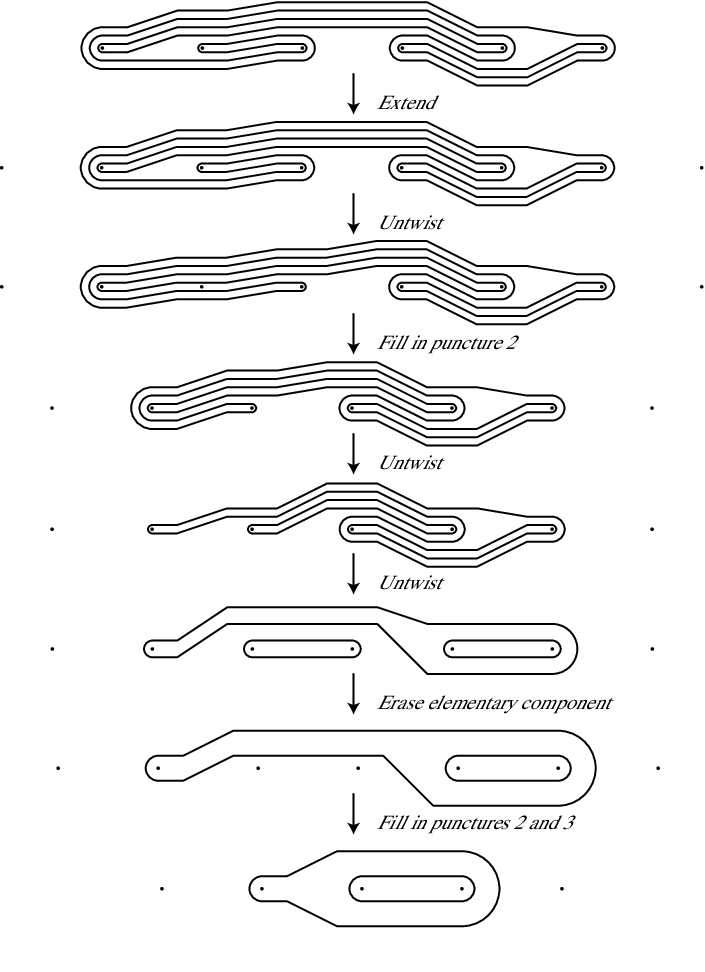
Figure 2: An example of the algorithm - 8.
Number of components: we have ; ; and (corresponding to the fact that our final lamination has one component bounding a disk containing the three central punctures).
Therefore .
References
- [1] E. Artin, Theory of braids, Ann. of Math. (2) 48 (1947), 101–126.
- [2] J. S. Birman, Braids, links, and mapping class groups, Princeton University Press, Princeton, N.J., 1974, Annals of Mathematics Studies, No. 82.
- [3] P. Dehornoy, I. Dynnikov, D. Rolfsen, and B. Wiest, Ordering braids, Mathematical Surveys and Monographs, vol. 148, American Mathematical Society, Providence, RI, 2008.
- [4] I. Dynnikov, On a Yang-Baxter mapping and the Dehornoy ordering, Uspekhi Mat. Nauk 57 (2002), no. 3(345), 151–152.
- [5] I. Dynnikov and B. Wiest, On the complexity of braids, J. Eur. Math. Soc. (JEMS) 9 (2007), no. 4, 801–840.
- [6] A. Haas and P. Susskind, The connectivity of multicurves determined by integral weight train tracks, Trans. Amer. Math. Soc. 329 (1992), no. 2, 637–652.
- [7] T. Hall and S. Ö. Yurttaş, On the topological entropy of families of braids, Topology Appl. 156 (2009), no. 8, 1554–1564.
- [8] J-O. Moussafir, On computing the entropy of braids, Funct. Anal. Other Math. 1 (2006), no. 1, 37–46.
- [9] R. C. Penner and J. L. Harer, Combinatorics of train tracks, Annals of Mathematics Studies, vol. 125, Princeton University Press, Princeton, NJ, 1992.
- [10] S. Ö. Yurttaş, Geometric intersection of curves on punctured disks, Journal of the Mathematical Society of Japan 65 (2013), no. 4, 1554–1564.