Estimation of Kullback-Leibler losses for noisy recovery problems within the exponential family
Abstract
We address the question of estimating Kullback-Leibler losses rather than squared losses in recovery problems where the noise is distributed within the exponential family. Inspired by Stein unbiased risk estimator (SURE), we exhibit conditions under which these losses can be unbiasedly estimated or estimated with a controlled bias. Simulations on parameter selection problems in applications to image denoising and variable selection with Gamma and Poisson noises illustrate the interest of Kullback-Leibler losses and the proposed estimators.
keywords
[class=MSC] Primary 62G05 , 62F10 ; secondary 62J12keywords
Stein unbiased risk estimator , Model selection , Kullback-Leibler divergence , Exponential familyIMB, CNRS, Université de Bordeaux, Bordeaux INP
351 cours de la Libération, F-33405 Talence, France
??
Contents
1 Introduction
We consider the problem of predicting an unknown -dimensional vector from its noisy measurements . Given a collection of parametric predictors of , we focus on the selection of the predictor that minimizes the discrepancy with the unknown vector . For instance, this includes the problem of selecting the best predictors from the set of Least Absolute Shrinkage and Selection Operator (LASSO) solutions [44] obtained for all possible choices of regularization parameters. To this end, the common approach is to select that minimizes an unbiased estimate of the expected squared loss , typically, with the Stein unbiased risk estimator (SURE) [43]. Such estimators are classically built on some statistical modeling of the noise, e.g., as being distributed within the exponential family. In this context, we investigate the interest of going beyond squared losses by rather estimating a loss function grounded on an information based criterion, namely, the Kullback-Leibler divergence. We will first recall some basic properties of the exponential family, give a quick review on risk estimation and motivate the use of the Kullback-Leibler divergence.
| Distribution law | ||||
|---|---|---|---|---|
| Gaussian () | ||||
| Gamma () | ||||
| Poisson | ||||
| Binomial () | ||||
| , | ||||
| Negative Binomial () | ||||
| , | ||||
Exponential family.
We assume that in the aforementioned recovery problem the noise distribution belongs to the exponential family. Formally, the recovery problem can be reparametrized using two one-to-one mappings and such that has a probability measure characterized by a probability density or mass function with respect to the Lebesgue measure of the following form
| (1.1) |
where . The distribution is said to be within the natural exponential family. We call the natural parameter, a sufficient statistic for , the base measure, and the log-partition function. Classical and important properties of the exponential family include that is convex, and (see, e.g., [3]). Here and in the following, denotes the expectation of the random vector with respect to the measure , and is its so-called variance-covariance matrix.
Without loss of generality, we consider that is a minimal sufficient statistic. As a consequence, is one-to-one and we can choose as the canonical link function satisfying (as coined in the language of generalized linear models). An immediate consequence is that has expectation and its variance is a function of given by where . The function is the so-called variance function (see, e.g., [36]), also known as the noise level function (in the language of signal processing).
Table 1 gives five examples of univariate distributions of the exponential family – two of them are defined in a continuous domain, the other three are defined in a discrete domain.
Risk estimation.
We now assume that the predictor of is a function of only, hence, we write it , and we focus on estimating the loss associated to with respect to . When the noise has a Gaussian distribution with independent entries, SURE [43] can be used to estimate the mean squared error (MSE), or in short the risk, defined as: . The resulting estimator, being independent on the unknown predictor , can serve in practice as an objective for parameter selection. Eldar [15] builds on Stein’s lemma [43], a generalization of SURE valid for some continuous distributions of the exponential family. It provides an unbiased estimate of the “natural” risk, defined as: , i.e., the risk with respect to . In the same vein, when the distribution is discrete, Hudson [26] provides another result for estimating the “exp-natural” risk: , i.e., the risk with respect to , where is the entry-wise exponential. As is assumed one-to-one, there is no doubt that if such loss functions cancel then . In this sense, they provide good objectives for selecting . However, within a family of parametric predictors and without strong assumptions on , such a loss function might never cancel. In such a case, it becomes unclear what its minimization leads it to select, all the more when or are non-linear. Furthermore, even when they are linear (e.g., for Poisson noise), minimizing might not even be relevant as it does not compensate for the heteroscedasticity of the noise (this will be made clear in our experiments). Estimating the reweighted or Mahanalobis risk given by could be more relevant in this case, but its estimation is more intricate.
Kullback-Leibler divergence.
The Kullback-Leibler (KL) divergence [27] is a measure of information loss when an alternative distribution is used to approximate the underlying one . Its formal definition is given by . Unlike squared losses, it does not measure the discrepancy between an unknown parameter and its estimate, but between the unknown distribution of and its estimate . As a consequence, it is invariant with one-to-one reparametrization of the parameters and, hence, becomes a serious competitor to squared losses. Remark that it is also invariant under one-to-one transformations of because such transforms do not affect the quantity of information carried by . Interestingly, provided and belongs to the same member of the natural exponential family respectively with parameters and , the KL divergence can be written in terms of the Bregman divergence associated with for points and , i.e.,
| (1.2) |
While squared losses are defined irrespective of the noise distribution, the KL divergence adjusts its penalty with respect to the scales and the shapes of the deviations. In particular, it accounts for heteroscedasticity.
Contributions.
In this paper, we address the problem of estimating KL losses, i.e., losses based on the KL divergence. As it is a non symmetric discrepancy measure, we can define two KL loss functions. The first one
| (MKLA) |
will be referred to as the mean KL analysis loss as it can be given the following interpretation: “how well might explain independent copies of ”. The mean KL analysis loss is inherent to many statistical problems as it takes as reference the true underlying distribution. It is at the heart of the maximum likelihood estimator and is typically involved in non-parametric density estimation, oracle inequalities, mini-max control, etc. (see, e.g., [22, 17, 41]). The second one will be referred to as the mean KL synthesis loss given by
| (MKLS) |
which can be given the following interpretation: “how well might generate independent copies of ”. The mean KL synthesis loss has also been considered in different statistical studies. For instance, the authors of [47] consider this loss function to design a James Stein-like shrinkage predictor. Hannig and Lee address a very similar problem to ours, by designing a consistent estimator of used as an objective for bandwidth selection in kernel smoothing problems subject to Gamma [24] and Poisson noise [25]. Table 2 gives a summary of our contributions. It highlights which loss can be estimated and under which conditions of the exponential family. The main contributions of our paper are:
- 1.
provided and the base measure are both weakly differentiable, can be unbiasedly estimated (Theorem 4.1),
- 2.
for any mapping , can be unbiasedly estimated for Poisson variates (Theorem 4.2),
- 3.
provided is times differentiable with bounded -th derivative, can be estimated with vanishing bias when results from a large sample mean of independent random vectors with finite -th order moments (Theorem 4.3).
It is worth mentioning that a symmetrized version of the mean Kullback-Leibler loss: , can be estimated as soon as and can both be estimated (e.g., for continuous distributions according to Table 2).
2 Risk estimation under Gaussian noise
This section recalls important properties of the and the definition of SURE under additive noise models of the form where and denotes the identity matrix.
Before turning to the unbiased estimation of , it is important to recall that for any additive models and zero-mean noise with variance , provided the following quantities exists, we have
| (2.1) |
where is the cross-covariance matrix between and . Equation (2.1) gives a variational interpretation of the minimization of the as the optimization of a trade-off between overfitting (first term) and complexity (second term). In fact, is a classical measure of the complexity of a statistical modeling procedure, known as the degrees of freedom (DOF), see, e.g., [13]. The DOF plays an important role in model validation and model selection rules, such as, Akaike information criteria (AIC) [1], Bayesian information criteria (BIC) [42], and the generalized cross-validation (GCV) [20].
For linear predictors of the form , (think of least-square or ridge regression), the DOF boils down to . As a consequence, the random quantity becomes an unbiased estimator of , that depends solely on without prior knowledge of . If is a projector, the DOF corresponds to the dimension of the target space, and we retrieve the well known Mallows’ statistic [35] as well as the aforementioned AIC. The SURE provides a generalization of these results that is not only restricted to linear predictors but can be applied to weakly differentiable mappings. A comprehensive account on weak differentiability can be found in e.g., [16, 18]. Let us now recall Stein’s lemma [43].
Lemma 1 (Stein lemma).
Assume is weakly differentiable with essentially bounded weak partial derivatives on and , then
A direct consequence of Stein’s Lemma, provided fulfills the assumptions of Lemma 1, is that
| (2.2) |
satisfies . Applications of SURE emerged for choosing the smoothing parameters in families of linear predictors [30] such as for model selection, ridge regression, smoothing splines, etc. After its introduction in the wavelet community with the SURE-Shrink algorithm [11], it has been widely used to various image restoration problems, e.g., with sparse regularizations [2, 38, 6, 37, 5, 32, 39] or with non-local filters [45, 12, 9, 46].
3 Risk estimation for the exponential family and beyond
In this section, we recall how SURE has been extended beyond Gaussian noises towards noises distributed within the natural exponential family.
Continuous exponential family.
We first consider continuous noise models, e.g., Gamma noise. To begin, we recall a well known result derived by Eldar [14], that can be traced back to Hudson11 1 In his paper, Hudson mentioned that Stein already knew about this result. in the case of independent entries [26], and that can be seen as a generalization of Stein’s lemma.
Lemma 2 (Generalized Stein’s lemma).
Assume is weakly differentiable with essentially bounded weak partial derivatives on and follows a distribution of the natural exponential family with natural parameter , provided is also weakly differentiable on , we have
Lemma 2, whose proof can be found in [14], provides an estimator of the dot product that solely depends on without reference to . As a consequence, the Generalized SURE (as coined by [14]) defined by
| (3.1) |
is an unbiased estimator of , i.e., , provided , and are weakly differentiable22 2 Eq. (3.1) is obtained by applying Lemma 2 on , and .. Note that omitting the last term in (3.1) leads to the seminal definition of GSURE given in [14] which provides an unbiased estimate of , even though is not weakly differentiable.
The GSURE can be specified for Gaussian noise, and in this case and the “natural” risk boils down to the risk as . In general, such a linear relationship between the ‘‘natural’’ risk and the risk of interest might not be met. For instance, under Gamma noise33 3 A random variable follows a Gamma distribution with scale parameter if it results from the mean of independent and identically distributed exponential random variables. For this reason, is often referred to as the number of looks and controls the spread of the distribution as . This distribution is widely used to describe fluctuations of speckle in coherent laser imagery [21]. with scale parameter (see Table 1), with expectation and independent entries, the GSURE reads as
| (3.2) |
which, as soon as and fulfills the assumptions of Lemma 2, unbiasedly estimates , where is the entry-wise inversion44 4 implies that and are weakly differentiable. By omitting the last term of GSURE, an unbiased estimate of is obtained as soon as .. We will see in practice that minima of can strongly depart from those of interest. As the GSURE can only measure discrepancy in the “natural” parameter space, its applicability in real scenarios can thus be seriously limited.
Discrete exponential family.
We now consider discrete noises distributed within the natural exponential family, e.g., Poisson or binomial. Before turning to the general result, let us focus on Poisson noise with mean and independent entries for which the Poisson unbiased risk estimator (PURE) defined as
| (3.3) |
unbiasedly estimates , see, e.g., [7, 26]. The vector is defined as and for . The PURE is in fact the consequence of the following lemma also due to Hudson [26].
Lemma 3 (Hudson’s lemma).
Assume follows a discrete distribution on of the natural exponential family with natural parameter , then
holds for every mapping where is the entry-wise exponential.
Hudson’s lemma provides an estimator of the dot product that solely depends on without reference to the parameter . As a consequence, we can define a Generalized PURE (GPURE) as
| (3.4) |
which unbiasedly estimates for the discrete natural exponential family55 5 Eq. (3.4) is obtained by applying three times Lemma 3. .
As for GSURE, GPURE cannot in general measure discrepancy in the parameter space of interest, and for this reason, its applicability in real scenarios can also be limited. However, under Poisson noise, the “exp-natural” space coincides with the parameter space of interest as , hence, leading to the PURE. Another interesting case, already investigated in [26], is the one of noise with a negative binomial distribution with mean and independent entries, for which the “exp-natural” space does not match with the one of but with the one of the underlying probability vector as defined in Table 1 (we have ). In such a case, GPURE reads, for , as
| (3.5) |
and is an unbiased estimator of .
Other related works.
It is worth mentioning that there have been several works focusing on estimating mean squared errors in other scenarios. For instance, when has an elliptical-contoured distribution with a finite known covariance matrix , the works of [28, 23] provide a generalization of Stein’s lemma that can also be used to estimate the risk associated to . In [40], the authors provide a versatile approach that provides unbiased risk estimators in many cases, including, all members of the exponential family (continuous or discrete), the Cauchy distribution, the Laplace distribution, and the uniform distribution [40]. The authors of [33] use a similar approach to design such an estimator in the case of the non-centered distribution [33].
4 Kullback-Leibler loss estimation for the exponential family
We now turn to our first contribution that provides, for continuous distributions of the natural exponential family, an unbiased estimator of the Kullback-Leibler synthesis loss.
Theorem 4.1 (Stein Unbiased KLS estimator).
Assume is weakly differentiable with essentially bounded weak partial derivatives on and follows a distribution of the natural exponential family with natural parameter , provided is weakly differentiable on , the following
where , is an unbiased estimator of .
Proof.
As GSURE, SUKLS can be specified for Gaussian noise, and in this case and the Kullback-Leibler synthesis loss boils down to the risk as . More interestingly, consider the following example of Gamma noise.
Example 1.
Under Gamma noise with expectation , shape parameter (as defined in Table 1) and independent entries, SUKLS reads as
| (4.2) |
which, up to a constant, and provided , unbiasedly estimates
| (4.3) |
In our experiments,
we will see that minimizing (or its SUKLS estimate)
leads to relevant selections, unlike
minimizing (or its GSURE estimate).
Note that the authors of [24] have proposed
a consistent estimator of when
(they did not study the case where ), their estimator
has been however designed only for kernel smoothing problems.
Theorem 4.1 is a straightforward application of Lemma 2 that applies since depends only on through a dot product for some mappings . For discrete distributions, Lemma 3 only provides an estimate of and hence cannot be applied to estimate . Alternatively, we can focus on estimating the Kullback-Leibler analysis loss . To this end, a formula that provides an estimate of for some mappings is needed. Of course, if for some continuous distributions, Lemma 2 applies and can be used to design an estimator of . However, the only distribution satisfying is the normal distribution, for which SURE can already be used to estimate . More interestingly, if for some discrete distributions, Lemma 3 applies and can be used to design an unbiased estimator of . The Poisson distribution satisfies this relation leading us to state the following theorem.
Theorem 4.2 (Poisson Unbiased KLA estimator).
Assume follows a Poisson distribution with expectation and independent entries, then
is an unbiased estimator of where
and is the entry-wise logarithm.
Proof.
With such results at hand, only the Poisson distribution admits an unbiased estimator of the mean Kullback-Leibler analysis loss. In order to design an estimator of for a larger class of natural exponential distributions, we will make use of the following proposition.
Proposition 1.
For any probability density or mass function of the natural exponential family of parameter , the Kullback-Leibler analysis loss associated to can be decomposed as follows
Proof.
Subtracting and adding in the MKLA definition leads to
As and , this concludes the proof. ∎
In the same vein as for the decomposition (2.1), Proposition 1 provides a variational interpretation of the minimization of , valid for noise distributions within the exponential family. Minimizing leads to a maximum a posteriori selection promoting faithful models with low complexity. It boils down to (2.1) when specified for Gaussian noise. As for the , the fidelity term can always be unbiasedly estimated, up to an additive constant, without knowledge of . Only the complexity term , which generalizes the notion of degrees of freedom, is required to be estimated. Except for the Poisson distribution, none of the previous lemmas can be applied to unbiasedly estimate this term. However, we will show that it can be biasedly estimated, with vanishing bias depending on both the “smoothness” of and the behavior of the moments of . Towards this goal, let us first recall the Delta method.
Lemma 4 (Delta method).
Let , , where is an infinite sequence of independent and identically distributed random vectors in with , and finite moments up to order . Let be times totally differentiable with bounded -th derivative, then
Lemma 4 is a direct -dimensional extension of [29] (Theorem 5.1a, page 109), that allows us to introduce our biased estimator of .
Theorem 4.3 (Delta KLA estimator).
Let , , where is an infinite sequence of independent random vectors in identically distributed within the natural exponential family with natural parameter , log-partition function , expectation , variance function and finite moments up to order . As a result, the distribution of is also in the natural exponential family parametrized by with log-partition function , expectation and variance function . Provided reads as , and is times totally differentiable with bounded -th derivative, then
where is the KL analysis loss associated to with respect to .
Proof.
It is worth mentioning that Theorem 4.3 can be applied to Gaussian noise, with DKLA boiling down to SURE, as . However, the conclusion is not as strong, as by virtue of Lemma 1, DKLA would be in fact an unbiased estimator provided only that is weakly differentiable. More interestingly, consider the two following examples.
Example 2.
Gamma random vectors with expectation and shape parameter (as defined in Table 1) results from the sample mean of independent exponential random vectors with expectation (entries of the vectors are supposed to be independent). As exponential random vectors have finite moments, provided is sufficiently smooth and since is continuously differentiable in , Theorem 4.3 applies and we get
| (4.9) | ||||
Example 3.
Consider the sample mean of independent Poisson random vectors with expectation . We have that , for all , belongs to the natural exponential family with and (entries of the vectors are supposed to be independent). As Poisson random vectors have finite moments, provided is sufficiently smooth and since is continuously differentiable in , Theorem 4.3 applies and we get
| (4.10) | ||||
Interestingly, remark that , as soon as we have both and .
5 Reliability study
In this section, we aim at studying and comparing the sensitivity of the previously studied risk estimators. Little is known about the variance of SURE: . It is in general an intricate problem and some studies [37, 31] focus instead on the reliability where (note that ). Here, we do not aim at providing tight bounds on the reliability as this would require specific extra assumptions for each pair of loss functions and estimators. The next proposition provides only crude bounds on the reliability of each estimator.
Proposition 2.
Assume is weakly differentiable. Then, provided the following quantities are finite, we have
where (note that ), and is defined similarly. The over-line refers to quantities for which additive constant with respect to are skipped, e.g., and .
Proof.
This is a straightforward consequence of Cauchy-Schwartz’s inequality. ∎
Proposition 2 allows us to compare the relative sensitivities of the different estimators. Comparing GSURE and SUKLS, one can notice that the bounds are similar but the first one is controlled by while the second one is controlled by . While it is difficult to make a general statement, we believe SUKLS estimates might be more stable than GSURE since has usually better control than , given the non-linearity of the canonical link function .
6 Implementation details for the proposed estimators
In this section, we explain how the proposed risk estimators
can be evaluated in practice within a reasonable computation time.
All risk estimators designed for continuous distributions rely on the computation of for some mappings and . For instance, SURE requires to compute such a a quantity with and (see eq. (2.2)). In general, the computation of these terms requires at least operations and thus prevents the use of such risk estimators in practice. Fortunately, following [19, 38], we can approximate such terms by using Monte-Carlo simulations, thanks to the following relation
| (6.1) |
where the directional derivatives in the direction
can be computed by using finite differences or algorithm differentiations
as described in [10].
This leads in general to a much faster evaluation in operations.
In the Poisson setting, risk estimators rely on the computation of for some mapping . For instance, PUKLA requires to compute such a quantity with (see Theorem (4.2)). Again, the computation of such terms requires at least operations in general. Based on first order expansions, we have empirically chosen to perform Monte-Carlo simulations on the following approximation
| (6.2) |
where is Bernoulli distributed with . In our numerical experiments, this approximation led to operations and satisfactory results even though was chosen to be non-linear. This approximation clearly deserves more attention but is considered here to be beyond the scope of this study.
7 Numerical experiments
In this section, we will perform numerical experiments showing the interest of the proposed Kullback-Leibler risk estimators in two different applications.
7.1 Application to image denoising
We first consider that and are dimensional vectors representing images on a discrete grid of pixels, such that entries with index are located at pixel location . A realization of represents a noisy observation of the image . The estimate of is a denoised version of .
Performance evaluation.
In order to evaluate the proposed loss functions and their estimates, visual inspection will be considered to assess the image quality in terms of noise variance reduction and image content preservation. In order to provide an objective measure of performance, taking into account heteroscedasticity and tails of the noise, we will evaluate the mean normalized absolute deviation error defined as . The MNAE measures to which extent might belong to a confident interval around with dispersion related to . The MNAE is expected to be when , and should get closer to when improves on itself.
Simulations in linear filtering.
We consider here that is the linear filter
| (7.1) |
where
is a circulant matrix encoding a discrete convolution with a Gaussian kernel of bandwidth .
In this context,
we will evaluate the relevance
of the different proposed loss functions and their estimates as objectives
to select a bandwidth offering a satisfying denoising.


Figure 1 gives an example of a noisy observation of an image representing fingerprints whose pixel values are independently corrupted by Gamma noise with shape parameter . We have evaluated the relevance of the natural risk given by , and in selecting the bandwidth . Visual inspection of the results obtained at the optimal bandwidth for each criterion shows that the natural risk fails in selecting a relevant bandwidth while and both provide a better trade-off. The natural risk strongly penalizes small discrepancies at the lowest intensities while not being sensitive enough for discrepancies at higher intensities. As the noisy image has several isolated pixel values approaching , the natural risk will strongly penalize smoothing effects of such isolated structures preventing satisfying noise variance reduction. The Kullback-Leibler loss functions take into account that Gamma noise has a constant signal to noise ratio. Hence, it does not favor the restoration of either bright or dark structures more, allowing satisfying smoothing for both, as assessed by the MNAE. Finally, estimators of these loss functions with respectively GSURE, SUKLS and DKLA are given. Note that for , the Gamma distribution is far from reaching the asymptotic conditions of Theorem 4.3. As a result, bias is not negligible (it becomes obvious for the lowest values of in Figure 1.h). Nevertheless, minimizing DKLA can still provide an accurate location of the optimal parameter for .
Figure 2 reproduces the same experiment but with Gamma noise with , i.e., with a much better signal to noise ratio. Interestingly, the bias of DKLA gets much smaller than in the previous experiment. This was indeed expected as with , the Gamma distribution fulfills much better the asymptotic conditions of Theorem 4.3. Remark that MNAE values are still in favor of Kullback-Leibler objectives, but the gains are much smaller. In fact, all MNAE values get closer to since noise reduction with signal preservation using linear filtering becomes much harder in such a low signal to noise ratio setting.


Simulations in non-linear filtering.
We consider here that is the non-local filter [4] defined by
| (7.2) |
where is a linear operator extracting a patch
(a small window of fixed size) at location ,
is a dissimilarity measure (infinitely differentiable and adapted to the exponential family following
[8])
and a bandwidth parameter.
Remark as depends on , is non-linear. In this context,
we will evaluate again the relevance
of the proposed loss functions and their estimates as objectives
to select the bandwidth .
Figure 3 gives an example of a noisy observation
of an image representing a bright two dimensional chirp signal shaded gradually into a dark homogeneous region.
The noisy observation is contaminated by noise following a Gamma
distribution with shape parameter .
We have again evaluated the relevance of the natural risk
given by ,
and in selecting the bandwidth parameter.
Visual inspection of the results obtained at the
optimal bandwidth for each criterion shows that the natural risk fails in selecting
a relevant bandwidth while and both provide more satisfying results.
As the image is very smooth in the darker region,
the natural risk favors strong variance reduction
leading to a strong smoothing of the texture in the brightest area.
Again, the Kullback-Leibler loss functions find a good trade-off preserving simultaneously
the bright texture and reducing the noise in the dark homogeneous region, as assessed by the MNAE.
Finally, estimators of these loss functions with respectively GSURE, SUKLS and DKLA are given.
Figure 4 gives a similar example where the image represents a two dimensional chirp signal shaded gradually into a bright homogeneous region. The image is displayed in log-scale to better assess the variations of the texture in the darkest region. The noisy observation is corrupted by independent noise following a Poisson distribution. We have evaluated the relevance of the risks , and in selecting the bandwidth parameter. Visual inspection of shows that darker regions are more affected by noise than brighter ones. This is due to the fact that Poisson corruptions lead to a signal to noise ratio evolving as . It follows that the essentially penalizes the residual variance of the brightest region hence leading to a strong smoothing of the texture in the darkest area. Again, Kullback-Leibler losses lead to selecting a more relevant bandwidth, smoothing less the brightest area but preserving better the texture, as assessed by the MNAE. Finally, estimators of the with PURE and with PUKLA and DKLA are given. Note that estimators of are not available for non-local filtering under Poisson noise.
7.2 Application to variable selection
We now consider the problem of variable selection in linear regression problems, i.e., in finding the non-zero components of a vector that fulfills the assumption that an observed vector has expectation where is the so-called design matrix. To this aim, we consider the Least Absolute Shrinkage and Selection Operator (LASSO) [44] given, for , by
In this case the predictor is given by . The LASSO is known to promote sparse solutions, i.e., such that the number of non-zero entries of is small compared to . The level of sparsity is indirectly controlled by the regularization parameter , the larger is, the sparser will be. Finding the optimal parameter , and then selecting the relevant variables (columns of ) explaining , is a challenging problem that can be addressed by minimizing an estimator of the risk. In this context, we will evaluate again the relevance of the different proposed loss functions and their estimates as objectives to select a regularization parameter offering a relevant selection of variables.
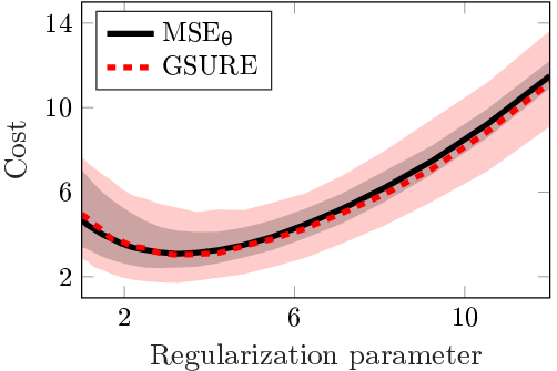
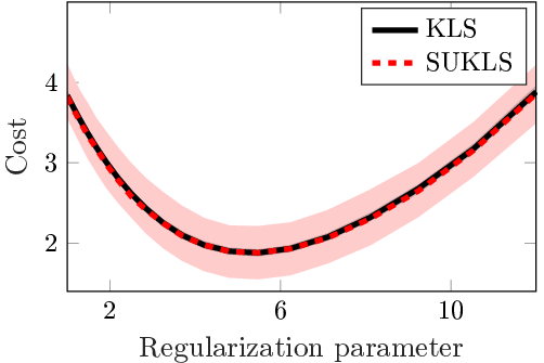
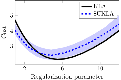
Figure 5 and Table 3 provide results obtained on such a linear regression problem where is an orthogonal matrix and . The vector was chosen such that of its entries are non-zero. We have generated independent realizations of using a Gamma distribution model with scale parameter . We have again evaluated the relevance of the natural risk given by , and in selecting the regularization parameter. Figure 5 shows the evolution of these objectives as a function of . It shows that KL objectives lead to selecting a larger parameter than with the natural risk. Performance in terms of average percentages of false negatives (FN: and ), false positives (FP: and ) and errors (FP or FN) are reported in Table 3. It shows that tuning the parameter with respect to KL objectives leads to lower numbers of errors than with the natural risk. One can observe that the subsequent LASSO estimators work at different trade-offs: KL objectives favor FN over FP, while the natural risk favors FP over FN. Finally, performances with estimators of with GSURE, with SUKLS, and MKLA with DKLA are also given. It can be observed that risk estimators offer in average comparable results than their oracle counterparts but have higher variance. Note that the LASSO is not differentiable, such that DKLA is not guaranteed to be asymptotically unbiased (as the conditions of Theorem 3 are not fulfilled), which explains the large discrepancies observed between the results obtained by MKLA and DKLA. Nevertheless, even though DKLA is not asymptotically unbiased in this case variable selections with the LASSO guided by DKLA still provides a good objective for variable selection, with similar results as if it was guided by the oracle MKLA objective.
| Errors | FN | FP | ||
| Correctly specified | ||||
| MSEθ | 34.64 3.09 | 11.36 1.28 | 23.27 4.36 | |
| GSURE | 34.00 4.34 | 11.74 1.95 | 22.25 6.26 | |
| MKLS | 26.24 0.28 | 15.68 0.16 | 10.56 0.23 | |
| SUKLS | 26.84 1.17 | 15.31 0.82 | 11.52 1.95 | |
| MKLA | 26.24 0.28 | 15.68 0.16 | 10.56 0.23 | |
| DKLA | 28.31 1.62 | 14.37 0.95 | 13.94 2.54 | |
| Misspecified | ||||
| GSURE | 35.94 4.44 | 10.93 1.81 | 25.01 6.22 | |
| SUKLS | 28.67 1.45 | 14.13 0.81 | 14.53 2.22 | |
| DKLA | 30.20 1.90 | 13.34 0.96 | 16.86 2.84 | |
A last important question is to know whether our risk estimators are robust against model misspecification, i.e., when the generative model (1.1) is only approximately known. Indeed, Lv and Liu [34] demonstrated the advantage of using KL divergence principle for model selection problems in both correctly specified and misspecified models. Along these lines, we have also shown in Table 3 the results obtained under misspecification. We have chosen to evaluate the performance of the LASSO guided by the aforementioned estimators of the risk when the shape parameter of the Gamma distribution is misestimated by a factor : . We found that the performance of all estimators drop in this case. Nevertheless, their relative performance are preserved: KL objectives lead to lower numbers of errors than with the natural risk.
8 Conclusion
We addressed the problem of using and estimating Kullback-Leibler losses for model selection in recovery problems involving noise distributed within the exponential family. Our conclusions are threefold: 1) Kullback-Leibler losses have shown empirically to be more relevant than squared losses for model selection in the considered scenarios; 2) Kullback-Leibler losses can be estimated in many cases unbiasedly or with controlled bias depending on the regularity of both the predictor and the noise; 3) Even though the estimation is subject to variance and bias, the subsequent selection has shown empirically to be close to the optimal one associated to the loss being estimated. Future works should focus on understanding under which conditions such a behavior can be guaranteed. This includes establishing tighter bounds on the reliability, consistency with respect to the data dimension and asymptotic optimality results for some given class of predictors. Estimation of Kullback-Leibler losses and other discrepancies (e.g., Battacharyya, Hellinger, Mahanalobis, Rényi or Wasserstein distances/divergences) beyond the exponential family and requiring less regularity on the predictor should also be investigated.
References
- [1] Akaike, H. (1973). Information theory and an extension of the maximum likelihood principle. In Second International Symposium on Information Theory 1 267–281. Springer Verlag.
- [2] [author] Blu, T.T. and Luisier, F.F. (2007). The SURE-LET approach to image denoising. IEEE Trans. Image Process. 16 2778–2786.
- [3] [author] Brown, Lawrence DL. D. (1986). Fundamentals of statistical exponential families with applications in statistical decision theory. Lecture Notes–Monograph Series i–279.
- [4] [author] Buades, A.A., Coll, B.B. and Morel, J. M.J. M. (2005). A Review of Image Denoising Algorithms, with a New One. Multiscale Modeling and Simulation 4 490.
- [5] [author] Cai, T. T.T. T. and Zhou, H. H.H. H. (2009). A data-driven block thresholding approach to wavelet estimation. The Annals of Statistics 37 569–595.
- [6] [author] Chaux, C.C., Duval, L.L., Benazza-Benyahia, A.A. and Pesquet, J-C.J.-C. (2008). A nonlinear Stein-based estimator for multichannel image denoising. IEEE Trans. on Signal Processing 56 3855–3870.
- [7] [author] Chen, L. H. Y.L. H. Y. (1975). Poisson approximation for dependent trials. The Annals of Probability 3 534–545.
- [8] [author] Deledalle, Charles-AlbanC.-A., Denis, LoïcL. and Tupin, FlorenceF. (2012). How to compare noisy patches? Patch similarity beyond Gaussian noise. International J. of Computer Vision 99 86–102.
- [9] [author] Deledalle, C. A.C. A., Duval, V.V. and Salmon, J.J. (2011). Non-local Methods with Shape-Adaptive Patches (NLM-SAP). J. of Mathematical Imaging and Vision 1-18.
- [10] [author] Deledalle, Charles-AlbanC.-A., Vaiter, SamuelS., Fadili, JalalJ. and Peyré, GabrielG. (2014). Stein Unbiased GrAdient estimator of the Risk (SUGAR) for multiple parameter selection. SIAM J. Imaging Sci. 7 2448–2487.
- [11] [author] Donoho, D. L.D. L. and Johnstone, I. M.I. M. (1995). Adapting to Unknown Smoothness Via Wavelet Shrinkage. J. of the American Statistical Association 90 1200–1224.
- [12] [author] Duval, V.V., Aujol, J-F.J.-F. and Gousseau, Y.Y. (2011). A bias-variance approach for the Non-Local Means. SIAM J. Imaging Sci. 4 760–788.
- [13] [author] Efron, B.B. (1986). How biased is the apparent error rate of a prediction rule? J. of the American Statistical Association 81 461–470.
- [14] [author] Eldar, Y. C.Y. C. (2009). Generalized SURE for exponential families: Applications to regularization. IEEE Trans. Signal Process. 57 471–481.
- [15] [author] Eldar, Y. C.Y. C. and Mishali, M.M. (2009). Robust recovery of signals from a structured union of subspaces. IEEE Trans. on Information Theory 55 5302–5316.
- [16] [author] Evans, L. C.L. C. and Gariepy, R. F.R. F. (1992). Measure theory and fine properties of functions. CRC Press.
- [17] [author] George, Edward IE. I., Liang, FengF. and Xu, XinyiX. (2006). Improved minimax predictive densities under Kullback-Leibler loss. The Annals of Statistics 78–91.
- [18] [author] Gilbarg, D.D. and Trudinger, N. S.N. S. (1998). Elliptic Partial Differential Equations of Second Order, 2nd ed. Classics in Mathematics 517. Springer.
- [19] [author] Girard, AA. (1989). A fast Monte-Carlo cross-validation procedure for large least squares problems with noisy data. Numerische Mathematik 56 1–23.
- [20] [author] Golub, G. H.G. H., Heath, M.M. and Wahba, G.G. (1979). Generalized cross-validation as a method for choosing a good ridge parameter. Technometrics 215–223.
- [21] [author] Goodman, Joseph WJ. W. (1976). Some fundamental properties of speckle. J. of the Optical Society of America 66 1145–1150.
- [22] [author] Hall, PeterP. (1987). On Kullback-Leibler loss and density estimation. The Annals of Statistics 1491–1519.
- [23] [author] Hamada, MahmoudM. and Valdez, Emiliano AE. A. (2008). CAPM and option pricing with elliptically contoured distributions. J. of Risk and Insurance 75 387–409.
- [24] [author] Hannig, JanJ. and Lee, ThomasT. (2004). Kernel smoothing of periodograms under Kullback–Leibler discrepancy. Signal Processing 84 1255–1266.
- [25] [author] Hannig, JanJ. and Lee, ThomasT. (2006). On Poisson signal estimation under Kullback–Leibler discrepancy and squared risk. J. of Statistical Planning and Inference 136 882–908.
- [26] [author] Hudson, H. M.H. M. (1978). A natural identity for exponential families with applications in multiparameter estimation. The Annals of Statistics 6 473–484.
- [27] [author] Kullback, SolomonS. and Leibler, Richard AR. A. (1951). On information and sufficiency. The Annals of Mathematical Statistics 79–86.
- [28] [author] Landsman, ZinoviyZ. and Nešlehová, JohannaJ. (2008). Stein’s Lemma for elliptical random vectors. J. of Multivariate Analysis 99 912–927.
- [29] [author] Lehmann, ELE. (1983). Theory of point estimation. Wiley publication.
- [30] [author] Li, K-C.K.-C. (1985). From Stein’s unbiased risk estimates to the method of generalized cross validation. The Annals of Statistics 13 1352–1377.
- [31] [author] Luisier, F.F. (2010). The SURE-LET approach to image denoising PhD thesis, École polytechnique fédérale de lausanne.
- [32] [author] Luisier, F.F., Blu, T.T. and Unser, M.M. (2010). SURE-LET for orthonormal wavelet-domain video denoising. IEEE Trans. on Circuits and Systems for Video Technology 20 913–919.
- [33] [author] Luisier, FlorianF., Blu, ThierryT. and Wolfe, Patrick JP. J. (2012). A CURE for noisy magnetic resonance images: Chi-square unbiased risk estimation. IEEE Trans. on Image Processing 21 3454–3466.
- [34] [author] Lv, JinchiJ. and Liu, Jun SJ. S. (2014). Model selection principles in misspecified models. J. of the Royal Statistical Society: Series B (Statistical Methodology) 76 141–167.
- [35] [author] Mallows, C. L.C. L. (1973). Some Comments on Cp. Technometrics 15 661–675.
- [36] [author] Morris, Carl NC. N. (1982). Natural exponential families with quadratic variance functions. The Annals of Statistics 65–80.
- [37] [author] Pesquet, J-C.J.-C., Benazza-Benyahia, A.A. and Chaux, C.C. (2009). A SURE Approach for Digital Signal/Image Deconvolution Problems. IEEE Trans. on Signal Processing 57 4616–4632.
- [38] [author] Ramani, S.S., Blu, T.T. and Unser, M.M. (2008). Monte-Carlo SURE: a black-box optimization of regularization parameters for general denoising algorithms. IEEE Trans. Image Process. 17 1540–1554.
- [39] [author] Ramani, S.S., Liu, Z.Z., Rosen, J.J., Nielsen, J-F.J.-F. and Fessler, J. AJ. A. (2012). Regularization parameter selection for nonlinear iterative image restoration and MRI reconstruction using GCV and SURE-based methods. IEEE Trans. on Image Processing 21 3659–3672.
- [40] Raphan, M. and Simoncelli, E. P. (2007). Learning to be Bayesian without supervision. In Advances in Neural Inf. Process. Syst. (NIPS) 19 1145–1152. MIT Press.
- [41] [author] Rigollet, PhilippeP. (2012). Kullback–Leibler aggregation and misspecified generalized linear models. The Annals of Statistics 40 639–665.
- [42] [author] Schwarz, G.G. (1978). Estimating the dimension of a model. The Annals of Statistics 6 461–464.
- [43] [author] Stein, C. M.C. M. (1981). Estimation of the Mean of a Multivariate Normal Distribution. The Annals of Statistics 9 1135–1151.
- [44] [author] Tibshirani, R.R. (1996). Regression shrinkage and selection via the Lasso. J. of the Royal Statistical Society. Series B. Methodological 58 267–288.
- [45] [author] Van De Ville, D.D. and Kocher, M.M. (2009). SURE-Based Non-Local Means. IEEE Signal Process. Lett. 16 973–976.
- [46] [author] Van De Ville, D.D. and Kocher, M.M. (2011). Non-local means with dimensionality reduction and SURE-based parameter selection. IEEE Trans. Image Process. 9 2683–2690.
- [47] [author] Yanagimoto, TakemiT. (1994). The Kullback-Leibler risk of the Stein estimator and the conditional MLE. Annals of the Institute of Statistical Mathematics 46 29–41.