Toward a 6/5 Bound for the Minimum Cost 2-Edge Connected Spanning Subgraph Problem Thanks: This research was partially supported by grants from the Natural Sciences and Engineering Research Council of Canada

Suppose the contrary, and let $G=(V,E)$ be the smallest counter-example for which $P(G)$ does not hold. Since $P(G)$ can be shown to be true directly for the unique graph $G$ with $|V|=4$ (see Figure 2, where bold lines indicate edges in $H_{i}$ and dotted lines indicate edges omitted), we can assume $|V|>4$.

For any edge $uv\in E$, let the unlabeled adjacent vertices at $u$ be $a$ and $b$, and the unlabeled adjacent vertices at $v$ be $c$ and $d$. Since $G$ is 3-edge connected, has no proper 3-edge cut and $|V|>4$, it follows that $a$, $b$, $c$ and $d$ are all distinct. This situation is illustrated on the left of Figure 3, where some incident edges are not shown for vertices $a$, $b$, $c$ and $d$. Removing $u$ and $v$ and their incident edges, and adding edges $ab$ and $cd$ yield a new cubic 3-edge connected graph $G^{\prime}=(V^{\prime},E^{\prime})$ with fewer vertices than $G$. Therefore, $P(G^{\prime})$ holds, so there exists a set of 2-edge connected spanning subgraphs $H_{i}$ with multipliers $\lambda_{i}$, $i=1,2,\dotsc,k$ such that $ab$ and $cd$ occur $\frac{4}{5}$ times overall in the convex combination. There are four patterns possible depending on the absence of $ab$ and $cd$ in $H_{i}$. These are indicated as patterns A, B, C and D in Figure 4, where an edge marked in bold indicates an edge which is in $H_{i}$, and a dotted edge indicates an edge which is not in $H_{i}$. For each pattern $Z$, we let $\lambda_{Z}$ represent the total occurrence of pattern $Z$ over all $H_{i}$ in the convex combination, i.e. $\lambda_{Z}=\sum(\lambda_{i}:\text{pattern }Z\text{ occurs in }H_{i})$.

Using the fact that $ab$ occurs exactly $\frac{4}{5}$ of the time, $cd$ occurs exactly $\frac{4}{5}$ of the time and $\lambda_{A}+\lambda_{B}+\lambda_{C}+\lambda_{D}=1$, it follows that

To create a convex combination of subgraphs for $G$, we create one or two 2-edge connected spanning subgraphs for each subgraph $H_{i}$ in the convex combination for $G^{\prime}$, as shown in Figure 4. In the case we use two, we use multiplier $\frac{\lambda_{i}}{2}$ for each, otherwise we use multiplier $\lambda_{i}$. In Figure 4 the resulting occurrences of the corresponding patterns in $G$ are indicated. Moreover, using (2) we have the occurrence of edges $au$ and $bu$ is $\frac{1}{2}(\lambda_{B}+\lambda_{D})+\lambda_{A}+\lambda_{C}=\frac{9}{10}$, the occurrence of $vc$ and $vd$ is $\frac{1}{2}(\lambda_{C}+\lambda_{D})+\lambda_{A}+\lambda_{B}=\frac{9}{10}$, and the occurrence of edge $uv$ is $\lambda_{B}+\lambda_{C}+\lambda_{D}=\frac{2}{5}-\lambda_{D}\leq\frac{2}{5}$, and all the other edges occur $\frac{4}{5}$ of the time (illustrated on the right of Figure 4). For simplicity, we will always work with exact fractions: should the occurrence of $uv$ be less than $\frac{2}{5}$ of the time, we will add it back to arbitrary subgraphs so that it appears exactly $\frac{2}{5}$ overall.

Applying the same technique for all edges $e\in E$ taken as edge $uv$ means that we have $m=|E|$ convex combinations, which we will refer to as $\mathbb{M}_{e}$ for each $e\in E$. Note that for any edge $f\in E$, $f$ occurs $\frac{2}{5}$ in $\mathbb{M}_{f}$, $f$ occurs $\frac{9}{10}$ in $\mathbb{M}_{e}$ for each of the four edges $e$ adjacent to $f$, and $f$ occurs $\frac{4}{5}$ in the rest of the convex combinations $\mathbb{M}_{e}$. We now take a convex combination of the $m$ convex combinations $\mathbb{M}_{e}$, $e\in E$, by multiplying every multiplier $\lambda_{i}$ used in these convex combinations by $\frac{1}{m}$. Summing the occurrence of every edge in this new convex combination gives

Therefore, we have a convex combination for $y^{*}$ for $G$ and $P(G)$ holds true, contradiction.

Notice that the ends of the three edges must be distinct since $G$ is 3-edge connected. In this case we contract each shore of the cut to a single vertex, to obtain graphs $G_{1}=(V_{1},E_{1})$ with pseudo-vertex $v_{1}$ and $G_{2}=(V_{2},E_{2})$ with pseudo-vertex $v_{2}$ (as shown in Figure 5). Both $G_{1}$ and $G_{2}$ are smaller than $G$, $|V_{1}|\geq 4$ and $|V_{2}|\geq 4$, so $P(G_{1})$ and $P(G_{2})$ hold. Moreover the patterns formed by the occurrence of the edges incident to $v_{1}$ and $v_{2}$ are unique and identical in the subgraphs in the corresponding convex combinations. For instance, exactly $\frac{1}{5}$ of the time, one of the incident edges will not be in the subgraph, on both sides of the cut, and this is true for each of the three incident edges. The remaining subgraphs contain all three incident edges. These constant patterns allow us to “glue” (reconnect the edges as there were before the inductive step) the subgraphs for $G_{1}$ and $G_{2}$ together, in such a way that identical patterns at $v_{1}$ and $v_{2}$ are matched. This results in a convex combination for $y^{*}$ that shows $P(G)$ holds, which gives a contradiction. ∎

If $G$ has only two half-triangles, then $Q(G,p)$ can be shown directly, using the $H_{i}$ and $\lambda_{i}$ shown in Figure 6, where edges represented by dotted lines are omitted, and $H_{1}$ and $H_{2}$ contain a multi-edge. Otherwise, let $G^{\prime}=(V^{\prime},E^{\prime})$ be the graph obtained from $G$ by shrinking each half-triangle to a pseudo-vertex. Graph $G^{\prime}$ is cubic and 3-edge connected and has $|V^{\prime}|\geq 4$, therefore by Lemma 2, $P(G^{\prime})$ holds, and yields a convex combination for $G^{\prime}$ with an edge occurrence of $\frac{4}{5}$ for all edges. Let the subgraphs in this convex combination be $H_{i}^{\prime},i=1,2,\ldots,k$ with multipliers $\lambda_{1}^{\prime},\lambda_{2}^{\prime},\ldots,\lambda_{k}^{\prime}$.

For each subgraph $H_{i}^{\prime}$ in the convex combination for $G^{\prime}$, the half-triangles (previously contracted to pseudo-vertices) will now be expanded to conclude the proof. We will add 1-edges and half-edges to each expanded $H_{i}^{\prime}$ in such a way that we create a convex combination for the original half-triangle graph $G$ that gives the required occurrence for each edge for the theorem. To accomplish this, for each triangle $T$ in each subgraph, we will add half-edges in patterns, where each pattern is used a fraction of the time (either $\frac{1}{2}$, or $\frac{1}{3}$). To facilitate this, we simply assume that we start with a new convex combination of $G^{\prime}$ which contains six copies of each subgraph $H_{i}^{\prime}$, where each copy has a coefficient of $\frac{\lambda_{i}^{\prime}}{6}$.

Now consider any triangle $T$ in $G$ and let its incident edges be $x$, $y$ and $z$. In the convex combination created for $G^{\prime}$, we have all three of these edges, or just two of these edges occur in each subgraph $H_{i}^{\prime}$. Let

Note that $\lambda_{xyz}^{\prime}+\lambda_{xy}^{\prime}+\lambda_{yz}^{\prime}+\lambda_{xz}^{\prime}=1$, and each of the 1-edges $x$, $y$ and $z$ occur $\frac{4}{5}$ of the time, thus each is missing exactly $\frac{1}{5}$ of the time. Thus

First we consider any expanded triangle $T$ which is not incident with edge $p$. For each subgraph $H_{i}^{\prime}$ in which all three edges $x$, $y$ and $z$ occur, we include two of the three edges in $T$ $\frac{1}{3}\lambda_{xyz}^{\prime}$ of the time. These patterns and their corresponding occurrences are illustrated in Figure 7, and result in an occurrence of $\frac{2}{3}\lambda_{xyz}^{\prime}=\frac{4}{15}$ for each edge of $T$ overall, by (3). Note that using each pattern one third of the time can be accomplished by using the patterns of Figure 7 for $T$ for two of the six copies of each $H_{i}^{\prime}$ where $x$, $y$ and $z$ occur. Then for each subgraph $H_{i}^{\prime}$ in which $z$ is omitted and $x$ and $y$ occur, we consider both triangle $T$ and the other triangle $T^{\prime}$ incident with $z$. In this case we include the edges in $T$ incident with $z$ $\frac{1}{2}\lambda_{xy}^{\prime}$ of the time, and the other edge in $T$ $\frac{1}{2}\lambda_{xy}^{\prime}$ of the time, and do the opposite in triangle $T^{\prime}$. In all cases we also include two copies of edge $z$. The patterns are illustrated in Figure 8 and result in an occurrence of $\frac{1}{2}\lambda_{xy}^{\prime}$ for each edge in $T$. Note that using each pattern half of the time can be accomplished by using each of the two patterns shown in Figure 8 for $T$ (and $T^{\prime}$) in three of the six copies of each $H_{i}^{\prime}$ in which $z$ is omitted. We do the same for the cases where $x$ or $y$ are omitted in $H_{i}^{\prime}$. The total occurrence of each half-edge in $T$ is

which by (3) is $\frac{17}{30}<\frac{3}{5}$. We can arbitrarily add back half-edges in the convex combinations to obtain an occurrence of exactly $\frac{3}{5}$ for these edges (for a complete illustration of the operations and the pattern occurrences, see Figure 9).

Note that each 1-edge which is not $p$ is now doubled whenever it was previously omitted, and thus occurs $\frac{6}{5}$ of the time. Also note that all patterns used in the expansion of the half-triangles ensure that the new multi-subgraphs created from the subgraphs $H_{i}^{\prime}$ for $G^{\prime}$ are also 2-edge connected and spanning in $G$, as required.

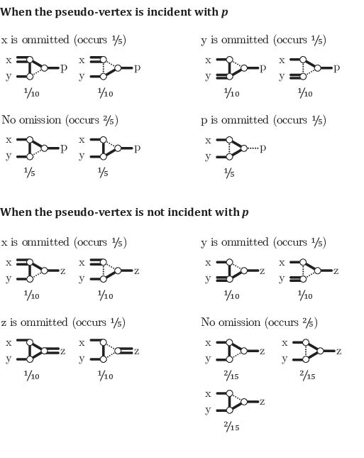
Next we consider any expanded triangle $T$ which is incident with edge $p$, and WLOG let $p=z$. For each subgraph $H_{i}$ in which all three edges $x$, $y$ and $p$ occur, we include two of the three edges in $T$ $\frac{1}{2}\lambda_{xyp}^{\prime}=\frac{1}{5}$ of the time, using the two patterns illustrated in Figure 10 (so we use each pattern in three of the six copies of $H_{i}^{\prime}$). Then for each subgraph $H_{i}^{\prime}$ in which $p$ is omitted and $x$ and $y$ occur we include the two edges of $T$ incident with $p$ in any of these operations. Recall this occurs $\lambda_{xy}^{\prime}=\frac{1}{5}$ of the time, by (3). Note that we do not double edge $p$. The total occurrence of each edge of $T$ is exactly $\frac{3}{5}$, and $p$ occurs exactly $\frac{4}{5}$ of the time (see Figure 9 for a complete illustration of these operations and the pattern occurrences).

We now have, over all cases, the half-edge occurrence is $\frac{3}{5}$, $p$ occurs $\frac{4}{5}$ of the time, and the occurrence of the other 1-edges is $\frac{6}{5}$. Furthermore, none of the 2-edge connected spanning multi-subgraphs use more than one copy of a half-edge or the edge $p$, and all of them use either one or two copies of a 1-edge. Thus $Q(G,p)$ holds.

Suppose the contrary, and let $G$ be the smallest counter-example for which $Q(G,p)$ does not hold. Let $G_{1}$, $G_{2}$ be the two sides of the cut $C$ in $G$, with $h$ and $j$ in $G_{1}$ and $i$ and $k$ in $G_{2}$, and WLOG choose $C$ such that $G_{1}+hj$ is 3-edge connected and does not contain $p$. By smaller example and Case 1, $Q(G_{1}+hj,hj)$ and $Q(G_{2}+ik,p)$ hold. We now “glue” together in the obvious way, the subgraphs in the convex combination for $G_{1}+hj$ where $hj$ is omitted with the subgraphs in the convex combination for $G_{2}+ik$ which have $ik$ doubled (both patterns occur $\frac{1}{5}$ of the time) by removing the double edge $ik$ and adding two copies of edges $hi$ and $jk$. Similarly, we glue the subgraphs for $G_{1}+hj$ and $G_{2}+ik$ where $hj$ and $ik$ occur as single edges in the subgraphs (both patterns occur $\frac{4}{5}$ of the time) by removing $hi$ and $ik$ and adding edges $hi$ and $jk$. We obtain $Q(G,p)$, contradiction. ∎

References

- [1] Alexander, A., Boyd, S., Elliott-Magwood, P., On the Integrality Gap of the 2-Edge Connected Subgraph Problem, Technical Report TR-2006-04, SITE, University of Ottawa, Ottawa, Canada.
- [2] Boyd, S., Fu, Y., Sun, Y., A 5/4-approximation for subcubic 2EC using circulations and obligated edges, Discrete Applied Mathematics, doi: 1016/j.dam.2015.10.014 (in press). a
- [3] Carr R., Ravi R., A new bound for the 2-edge connected subgraph problem, Proceedings of Integer Programming and Combinatorial Optimization (IPCO), Lecture Notes in Computer Science, Springer, 112-125, 1998.
- [4] Csaba, B., Karpinski, M., Krysta, P., Approximability of dense and sparse instances of minimum 2-connectivity, tsp and path problems, D. Eppstein (Ed.), SODA, ACM/SIAM, 74-83, 2002.
- [5] Frederickson, G. N., Ja’Ja’, J. On the relationship between the biconnectivity augmentation and travelling salesman problems, Theoretical Computer Science, 19, 189-201, 1982.
- [6] Jain, K., A factor 2 approximation algorithm for the Generalized Steiner Network Problem, Combinatorica 21 No 1, 39-60, 2001.
- [7] Sebő, A., Vygen, J., Shorter tours by nicer ears: 7/5 approximation for the graph-tsp, 3/2 for the path version, and 4/3 for two-edge-connected subgraphs, Combinatorica 34, 597-629, 2014.