Multiple scales approach to the Gas-Piston non-equilibrium themodynamics
2 Universitá degli Studi Roma tre, Dipartimento di Matematica e Fisica and Sezione INFN di Roma Tre
Abstract
The non-equilibrium thermodynamics of a gas inside a piston is a conceptually simple problem where analytic results are rare. For example, it is hard to find in the literature analytic formulas that describe the heat exchanged with the reservoir when the system either relaxes to equilibrium or is compressed over a finite time. In this paper we derive such kind of analytic formulas. To achieve this result, we take the equations derived by Cerino et al. [Phys. Rev. E 91, 032128] describing the dynamic evolution of a gas-piston system, we cast them in a dimensionless form and we solve the dimensionless equations with the multiple scales expansion method. With the approximated solutions we obtained, we express in a closed form the heat exchanged by the gas-piston system with the reservoir for a large class of relevant non-equilibrium situations.
1 Introduction
One of the irrefutable facts in learning thermodynamics and statistical mechanics is that, when facing the two topics for the first time, one has to get skilled in solving problems that involve gasses and pistons. This is due to historical reasons. One is that thermodynamics was initially developed to understand the phenomenology of steam engines. One other is that the first model where the macroscopic properties of a body were linked to its internal constituents is the kinetic theory of gasses by Maxwell and Boltzmann. More than one hundred years have now passed form the work of Maxwell and Boltzmann and thermodynamics and statistical mechanics have widely changed: from theories that describe equilibrium conditions only, they are slowly but steadily evolving to include non-equilibrium frameworks [15, 2, 30, 29, 7] and results [20, 14, 16, 28, 8]. However, gasses and pistons have never stopped playing a prominent role in such evolution as their nonequilibrium behavior is not yet fully understood. As a proof, Elliot Lieb stated that he would like to see solved the adiabatic piston problem [24]. It can be formulated as follow: we take an insulating canister with two gasses inside that are separated by a perfectly insulating moving piston. If the two gasses are initially at different pressures and temperatures, how is the equilibrium condition approached? It turns out that it’s easy to answer this question qualitatively [17], while quantitative answers are still a very active field of research [18, 9, 10]. Curiously enough, the adiabatic piston problem is very similar to another which is not that much investigated, although it involves a conceptually simpler system and it’s more relevant for applications. We consider the simplest thermodynamic machine: a perfect gas enclosed by a cylindrical canister with a movable piston and in contact with a heat reservoir (Figure 1). This system is simpler than the adiabatic piston as 1) only a single perfect gas is involved and 2) gas-reservoir heat exchanges are easily modeled microscopically [31]. Additionally, this device can be described by a limited set of macroscopic variables: the piston position , the gas internal temperature , the reservoir temperature and the external force applied on the piston. Among those variables, and can be changed according to some external time dependent protocol while and evolve as a consequence. It is worth to note that, in the adiabatic piston problem, the force exerted by the piston can never be considered as an external known function, as it is an internal variable.

One possible way to describe the time evolution of and is given in [11] through the following Gas-Piston equations11 1 An anonymous referee pointed out that our eq.(1a) and the original eq. A1 in [10] don’t have the same last term. Such discrepancy is due to a confirmed misprint[1] in [10]. (GPE)
| (1a) | ||||
| (1b) | ||||
where the upper dots denote time derivatives, is the mass of the piston, is the mass of a single gas molecule, is the total number of gas molecules, and is the complementary error function. Without going to much into details, these macroscopic equations are obtained by averaging microscopic properties with the aid of heavy assumptions. The first one is that the piston and each gas particle undergoes elastic collisions, so work is the energy exchanged in this way. The second assumption is that the velocity of a gas particle is randomly changed according to the Maxwell-Boltzmann distribution of the reservoir when reservoir-gas particle collisions occurs [31]. Heat is no more than the change in energy of the gas due to this collision mechanism. The third assumption is that the gas distribution is always Maxwellian although gas-reservoir and gas-piston collisions change the gas temperature over time. From a physical point of view, this third assumption rules out any shock-wave propagation, making the gas an efficient macroscopic dissipative medium [9].
If the solution of eq.(1) is known, it’s possible to compute the total energy of the system [11, 21], the work performed on the piston [29, 30]22 2 The sign conventions for and are the same used in [29], i.e. for heat given to the reservoir and for work applied on the system. and the heat exchanged with the reservoir as:
| (2a) | ||||
| (2b) | ||||
| (2c) | ||||
It is worth to note that is considered as a part of the total energy of the system. As a consequence, work must be defined as eq.(2b) [21].
In this paper we present eq.(1) in a new dimensionless form which allows to easily take the thermodynamic limits
| (3) |
and to isolate
| (4) |
as the only relevant free parameter[18]. Assuming that is small and that the external force is slowly-varying over time, we linearize eq.(1) and then proceed to an asymptotic expansion using the multiple scales method. This way we find and approximated solution of the linearized equations which contains all the relevant physical behaviors of the system. Furthermore we use the obtained solutions to build closed form expressions for the heat exchanged with the reservoir for two relevant non-equilibrium transformations, namely the relaxation toward equilibrium and the isothermal compression of a gas realized in a finite time. In the next Section we give an account of the multiple scales method and then proceed with the outline presented above.
2 Short review on multiple scales method
The history of the multiple scales method dates back to the 18th century from the works of by Lindstedt [25] and Poincaré [27], and was developed in its modern form in [23, 13]. The core of the method is to find asymptotic approximated solutions to a differential equation when the standard perturbation theory produces secular terms. During the years the multiple scales method has proven to be very useful in the construction of approximate solutions of differential equations and is now included in every textbook on perturbation theory [26, 3, 22, 19]. Such powerful method has found applications also in fields which seems not to have any correlation with such problems, for example in the theory of integrable systems [32, 5, 6, 4].
The key feature that allows the elimination of the secular terms is the introduction of fast-scale variables and slow-scales variables in a way that the dependence on the slow-scale variable will prevent the secularities. To be more precise, suppose that we are in the case of an ordinary differential equation with respect to the independent variable and a single dependent variable :
| (5) |
where the subscript means that we have some dependence on a small parameter . We now assume that has an asymptotic series of the form:
| (6) |
truncated at some positive integer , with . In the right hand side of (6) the dependence on the time variable appears trough the so called scales 33 3 If is a time variable, the scales are the characteristic time scales of . Similarly, if is a length variable, the scales are the characteristic length scales of . Intuitively, the scales isolate different behaviors inside eq. (5), e.g. in the damped harmonic oscillator they separate oscillations from the amplitude suppression. The number of scales to be introduced depends on the desired asymptotic approximation order: the expansion is guaranteed to be asymptotic until
| (7) |
is satisfied. The number of scales also sets the approximation error, in the sense that the maximum discrepancy from the complete solution
| (8) |
is , where is the time such that the condition (7) holds.
The mathematical structure of the scales is the most delicate point in the whole expansion method: it involves the knowledge of eq.(5) structure, and the constraint that they must be non-decreasing functions of which satisfy the condition:
| (9) |
We note that has to be sufficiently high not just to give a longer asymptotic range of validity of the expansion, but also to capture the behavior of the system.
The substitution (6) can be extended to all the derivatives of by differentiation, or more operatively by substituting
| (10) |
Substituting eq.(6) and all its derivatives in eq.(5), eventually expanding in Taylor series with respect to , we obtain a polynomial in which is identically equal to zero. We can then separately set to zero all the coefficients of -powers and obtain a system of partial differential equations. If the scales are correctly chosen, the -equation, will contain only and will depend just on . This will give raise to a solution depending on arbitrary functions of the remaining scales . Substituting into the -equation we use these arbitrary functions to prevent the birth of the secular terms in . Solving iteratively for the remaining one finally writes down the terms of the wanted expansion (6). In the case of high order expansions () sometimes the previous iterative method is not sufficient to completely specify the terms of the asymptotic series. In these cases the strategy of the suppression of the order mixing is adopted: it consist in eliminating from the -equation all the contributions coming from the arbitrary functions coming from lower orders solutions , , etc. This increases the accuracy of the first terms by reducing the amounts of corrective terms in [19].
3 Adimensionalization and expansion of the piston-gas equations
Going back to the main aim of this paper, we introduce a dimensionless version of eq.(1), namely
| (11a) | ||||
| (11b) | ||||
To obtain this expression we have introduced in eq.(1) the dimensionless quantities , , , and the dimensionless time via
| (12a) | ||||
| (12b) | ||||
| (12c) | ||||
| (12d) | ||||
| (12e) | ||||
where
| (13) |
and () is an arbitrary force (temperature) reference value. Similarly we write the dimensionless , and densities:
| (14a) | ||||
| (14b) | ||||
| (14c) | ||||
It is important to note that in eq.(11) and (14) the thermodynamic limit eq.(3) are already taken, provided that the gas-piston mass ration defined in eq.(4) is finite. We also note that (11) and (14) show an important property firstly observed in the related adiabatic piston problem [18]: the sole knowledge of is sufficient to describe the general features of the system while the remaining parameters appears as scaling factors. Following again [18] we also treat as a small perturbation parameter.
We now restrict ourselves to the case where the reservoir temperature is constant over time while evolves according to a given slow protocol. W.l.o.g, we take . can be considered slow if
| (15) |
The simplest way to satisfy eq.(15) is to take , which we assume from now on.
Since varies slowly, the equilibrium point of eq.(11), namely
| (16) |
is also slowly varying over time. Since we are interested in results of thermodynamic relevance, we are allowed to linearize eq.(11) around eq.(16), which yields
| (17a) | ||||
| (17b) | ||||
We call eq.(17) the Linearized Dimensionless Gas Piston Equations (LDGPE).
Being the LDPGE linear, we could expect an exact analytic solution. However Computer Algebra Systems like Macsima or Maple show that analytic solutions of the LDGPE are of no practical use or even impossible to express because they are too strongly dependent on value and on the functional form of .
The LDGPE equations (17) are a system of a second order equation coupled with a first order one. However we show that it can be treated as a single third order equation. We solve eq. (17a) for :
| (18) |
and then insert it into (17b) to obtain:
| (19) | ||||
where ′ stands for the differentiation with respect to the argument44 4 In general where is a dummy variable..
Since the force is slowly varying and we don’t want to treat just a particular case, we are naturally led to consider not a standard perturbative approach55 5 Expanding in the standard way requires to express as Taylor series, thus losing generality., but the multiple scales one.
The -perturbation is singular, i.e. if then (19) ceases to be a third order equation, but collapse into a second order one. Indeed from (19) it is clear that as the dominant term is given by:
| (20) |
which is just an harmonic oscillator with slowly varying frequency and slowly forcing . To avoid the singularity we just make an -scaling in and , with undetermined coefficients, i.e. . Substituting into (19) we found that we have to impose and ; putting we obtain:
| (21) | ||||
As can be easily seen now we have no singularity as and the dominant term is now a third order equation.
The next step is to introduce the time scales. It is easy to see that if we choose the trivial time scales
| (22) |
we end up with an asymptotic expansion which is identically zero, meaning that this choice is not correct. However, we can use the trivial time scales when the force . To construct the time scales in the general setting , we search a change of variables such that the term in eq.(21) reduces to the term for the case. Performing such change of variables we obtain:
| (23) | ||||
Since the term for is
| (24) |
we see that we have:
| (25) |
For the second scale we repeat the same procedure as implies an identically zero asymptotic behavior. Performing again such procedure we see that the second scale is . As third scale we can safely choose . In the end we have the following three scales:
| (26) |
It’s worth to note that, two different time scales faster that the external driving time scale are required for a full description of the system. Since the time scales of the multiple scales method are each one associated to a different physical phenomena, eq.(26) gives us a rigorous proof that is indeed a slow force if compared with the remaining fundamental time scales of the system. We will address to which phenomena and are related later in this paper. We note that the condition (9) is satisfied by the scales (26), but the requirement for them to be non-decreasing functions impose some restrictions on . We note that if function is always positive, then this requirement is automatically satisfied. Many cases of physical interests satisfies such positivity requirement and these will be discussed later in the paper.
Now we introduce the truncated expansion:
| (27) |
and substitute it into (21) with . Taking the coefficients with respect to to be zero, we found the following equations up to :
| (28a) | ||||
| (28b) | ||||
| (28c) | ||||
It is very easy to see that the solutions to these equations are weakly secular in the sense that, except in some notable cases, the convergence of expansion is ensured by the presence of exponentially decreasing functions. Therefore we adopt the strategy of the suppression of order mixing: we use the arbitrary functions in , …, to eliminate as much as possible the presence of , …, in the equations for , …, . At this point we notice that to give a complete characterization to the function , and it is not possible to just use the three equations above, but one must add terms up to . We omit the further three equations and all the calculations, since they are very long, but in fact trivial. The results of the calculations, once written in the original variable time scales
| (29) |
becomes:
| (30) |
Where:
| (31) | ||||
The part of the function is not displayed in its generality since it is very long and cumbersome, but we note that the writing means that has parametric dependence on the , and which are the constants of integration. In the next sections, while discussing some particular cases of , we show the specific forms it assumes.
We can construct a general formula for the expression of the asymptotic series for substituting eq.(30) into eq.(18):
| (32) |
We have then that the error on is of order since to have a better estimate on it, it is necessary the knowledge of the term.
A particularly interesting case arise when all the constants of integration are taken to be zero, , which, being the system linear, corresponds to the case when the initial condition is trivial and the system evolves according to the external forcing. Since the system is, in general, non-autonomous this is the dynamical equilibrium and is given by:
| (33) |
Notice that as was previously known [11] the contribution to the dynamical equilibrium solution is the same as that of the underlying forced harmonic oscillator (20). The first correction is then second order, while the next one will be at fourth66 6 We remark that to compute the complete expansion we needed six terms..
Upon differentiation with respect to from (33) we obtain the modified equilibrium conditions for and (the latter by using (32)). For the dynamical equilibrium we obtain from (32) the following very simple expression:
| (34) |
We remark that upon substituting the dynamical equilibrium reduces exactly to the usual equilibrium condition , and . We also note that eq.(33) and (34) can be derived as standard perturbation expansion assuming .
Since our starting hypothesis was that the original DGPE are in linear regime, it is particularly useful to express the initial conditions of the system not as generic, but as deviation from the dynamical equilibrium (33). Using (34) and (18) valued at we find the following values for the near equilibrium initial conditions for eq. (19):
| (35a) | ||||
| (35b) | ||||
| (35c) | ||||
Here , and are taken to be deviations from equilibrium eq. (33). This will give us the following values for the constants of integration:
| (36) | ||||
whereas and is left unspecified, meaning that it can be safely put to zero. We note that the initial conditions are satisfied exactly at , up to order at and up to order at . This is not an accident of our system, but is a standard feature of the multiple scales approach [22]. The fact that is not surprising. From eq. (32) it is quite clear that the first two orders and must vanish to get as initial condition .
Without the need for an explicit form of we can now give an intuitive meaning to the the three scales we introduced. The -scale is the fastest one and characterizes an exponential-relaxation of the system toward the equilibrium position given by (33). We notice from that this scale appears in as an term, giving very little contribution. We also note that, due to the presence of second order derivatives in eq.(32) the scale appears in as the leading order term. This means that the temperature of the gas can have deviations from equilibrium as large as and still rapidly converge to the equilibrium value. The -scale is the one at which the oscillations of the system are established. It is worth to note, that even if the system possess a clear dissipative behavior, the basic frequency of the system is unaltered adding the third scale meaning that, if any correction in the basic frequency exists, then it should be at least of order . In the -scale the exponential suppression of the oscillatory terms appears; this means that the oscillations are slowly modulated. Overall we see, under suitable assumption on the smallness of , that the approximated solution tends to the dynamical equilibrium solution (33) as which is coherent with a transient like behavior. We note that using only two time scales would have resulted in missing the modulation of the oscillation, leading to an erroneous result from both the physical and mathematical point of view. The previous considerations give us an a posteriori justification of the choice of using only three time scales, since all the above features describe well the behavior of the system from both a numerical and a physical point of view.
As a final recall on terminology we call from now on the truncated part of the expansion for at order given by (30), and we call the truncated part of the expansion for at order . The next two Sections are devoted to two particular examples of thermodynamic relevance which we will use to test the quality of as an approximated solution of the LDGPE and to derive new closed form expression of .
4 Relaxation to equilibrium
The first case under study is the one in which
| (37) |
with initial conditions
| (38) | ||||
This simple case encompasses all the situations where the gas and the piston relax from a given nonequilibrium condition to the thermodynamic equilibrium , , }. Substituting eq.(37) in eq.(30) and eq.(29), and then imposing that eq.(36) must hold, we obtain an approximated expression for the piston position
| (39) | ||||
with
| (40) | ||||
and nonzero integration constants
| (41) | ||||
In addition to the general properties of the scales inherited from eq.(30), eq.(39) shows two interesting properties. The first one is given by its general structure: being eq.(39) made of a constant plus two decaying functions, it thermalizes and it describes well the relaxation to equilibrium. The second property is that we are now able to address the physical phenomena to which () and () are related to. As a matter of fact, gives the suppression mechanism related to the mechanical damping the gas acts on the piston with a characteristic time of . On the other hand, gives a second suppression mechanism emerging from the indirect coupling of the piston with the reservoir with a characteristic time of . The fact that the piston-reservoir interaction is indirect is shown by the fact that this effect is in whereas in (where the gas-reservoir contact is direct) this effect is . This feature is not surprising, as the the temperature reservoir appears explicitly only in eq.(17b) and not in eq.(17a), but we are now able to describe quantitatively this phenomena.
To test the quality of as solution we note that the exponents of eq.(30) converge only if
| (42) |
which gives a more rigorous meaning to the small assumption. We then compute the differences
| (43) | |||
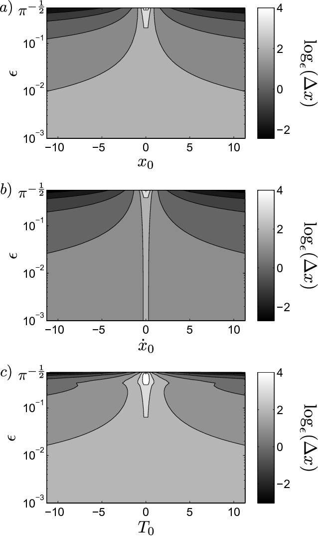
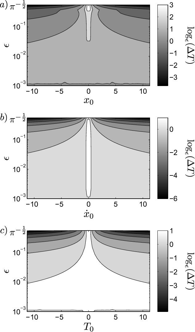
between the approximated and the numerical solutions of eq.(17) as functions of and one free initial condition while the remaining two are the equilibrium values (e.g. free, and ). Figure 2 and Figure 3 show that, for a wide range of values and initial conditions, is while is , which is consistent with the general properties of eq.(30) and eq.(32).
We now compute the heat produced while the system relaxes to equilibrium. Substituting eq.(37) and in eq.(14c), gives
| (44) |
Using now that and that , we obtain the approximate expression for the heat
| (45) |
where we evaluated and instead of using eq.(38). This expression describes the heat exchanged with the reservoir as a relaxation process takes place and is fully analytic: numerical evaluation becomes a trivial task, while using it for some formal calculations is likely to allow results to be expressed in a closed form.
5 Compression in a finite time
The second example we consider is the case in which the system, initially at equilibrium, undergoes a linear increase of the external force over a finite time and then relaxes to the new equilibrium condition. This encompasses all the isothermal compressions occurring in a finite time. W.l.o.g. this is modeled by taking
| (46) |
with initial conditions
| (47) | ||||
The additional parameters appearing in eq.(46) are the amount of force by which is increased and the constant which fixes the time-span . Substituting eq.(46) in eq.(30) and then imposing that eq.(47) must hold, we obtain after a long but straightforward calculation that, for ,
| (48) |
while for , the system relaxes and is given by an adjusted version of eq.(39) such that , and . We stress out that eq.(48) is valid up to order because it satisfies equilibrium boundary conditions. Consequently, the corresponding is valid up to .
At this point we can compute eq.(43) as functions of , and to investigate the quality of eq.(48). Since this parametric study does not yield results strikingly different from the ones we obtained for the relaxation case, we rather test the goodness of by looking at the heat produced during the gas compression. If we neglect heat exchanges at intermediate times, the net heat produced by this thermodynamic transformation is obtained by substitution of and eq.(46) into eq.(14c). After some simple calculations we obtain
| (49) | ||||
where we dropped and for compactness and the new dependence is to remind that the compression occurs for . Substituting here eq.(48) gives the approximated expression for the heat77 7 As in the previous case, and
| (50) | ||||
This formula is our main thermodynamic result: it estimates the heat produced by a perfect gas under the action of a finite-time compression. One interesting property of eq.(50) is that in the limit of quasi-static transformations, i.e. ,
| (51) |
This is exactly the value prescribed by Clausius theorem. As a consequence, the remaining terms of eq.(50) are contributions coming to the fact that the system is driven in a finite time. To have physical meaning, such contributions must be positive. This is a non-trivial requirement. However, the multiple scales method can be applied only if
| (52) | ||||
and, within these constrains, such positivity requirement is always satisfied.
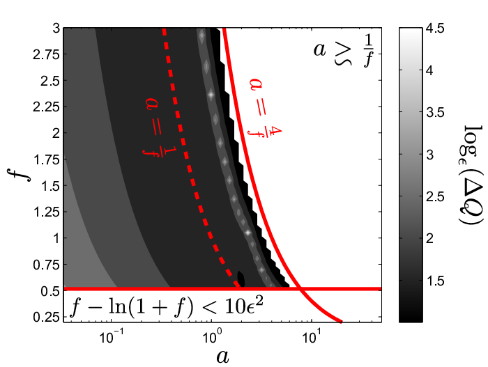
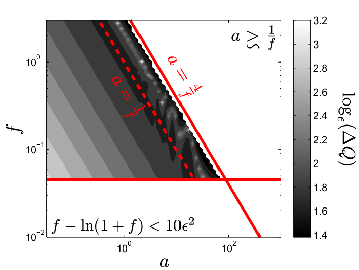
We note that eq.(52) is not the only validity constrain because the worst protocol with the functional form of eq.(46) is the one where the compression is instantaneous. This corresponds to take the limit in eq. (14c) with eq.(47) and yields the upper bound . Therefore we must have that . Since eq.(50) has an evaluation error of the order of , if the inequality
| (53) |
is not satisfied, the estimation error on eq.(50) is bigger than the energy region we want to investigate. Any result obtained with is then of no practical use. We therefore conclude that the validity region of eq.(50) is given by eq.(52) and eq.(53).
We conclude this section with a numerical study of eq.(50): we compute the difference
| (54) |
as functions of and for a given value. Figure 4 and 5 show the result obtained for and . From the picture it clearly appears that is within the constraints defined by eq.(52) and eq.(53). This proves that eq.(50) is a good analytical expression of the heat produced during a finite time compression of a perfect gas.
6 Conclusions and future developments
In this paper we focused on the LDGPE derived in [11] to describe the dynamical evolution of a gas enclosed by a piston and in contact with a heat reservoir. In particular, we showed that the LDGPE have an approximated analytic solution when the temperature of the reservoir is fixed and the force applied on the piston varies according to a general force protocol. To derive such result we used the multiple scales expansion method. Although this is valid only within some constraints, we can use the approximated solutions to describe the thermodynamics of fundamental nonequilibrium processes. Our main result is that we are now able to compute in a closed form the heat produced when the gas-piston system 1) relaxes toward equilibrium, and 2) undergoes an isothermal compression in a finite time. As the derivation of analytic heat relations through the multiple scales method turned out to be quite straightforward, we believe that this perturbative technique could be useful in understanding finite time thermodynamics.
An issue that deserves futures investigations is the following: we already stated that eq.(50) is valid when . Nonetheless, it’s clear that an instantaneous compression () produces heat only because the system relaxes toward the new equilibrium condition. It is not hard to prove by means of eq.(45) that . We thus have that eq.(30) allows to simultaneously describe the heat produced by an isothermal compression for both and . This gives us an hint that there could be a way to access the missing region by means of some well aimed multiple scales expansion. One other issue that can be treated with the multiple scales method is the study of the resonance of eq.(17). Since the system has a unitary characteristic frequency, this problem can be efficiently addressed with the multiple scales method [22, 19, 3] by choosing
| (55) |
which is small in amplitude but not slow anymore. We also note that our results are a direct consequence of linearity of the LDGPE. However we are interested to derive a multiple scales expansion also for the DGPE. It is clear to the reader that this problem is far much difficult from the linear one because 1) the system does not reduce to a single equation and 2) and need different scalings to avoid singularities.
We conclude by noting that if we restrict ourselves to dynamical equilibrium solutions we proved that it’s possible to compute the heat exchanged when also the reservoir temperature is slowly varying over time [12]. The price to pay is that we lose the characterization of transient behaviors. However, those can be accessed by a full multiple scales method where also .
Acknowledgments
We would like to thank L. Gammaitoni, A. Vulpiani and L. Cerino for the useful discussion on the topic. DC is supported by the European union (FPVII(2007-2013) under G.A. n.318287 LANDAUER). GG is supported by INFN IS-CSN4 Mathematical Methods of Nonlinear Physics.
References
- [1] private comunication with one of the authors.
- [2] R. Balescu. Equilibrium and Nonequilibrium Statistical Mechanics. Wiley-Blackwell, 1975.
- [3] C. M. Bender and S. A. Orszag. Advanced mathematical methods for scientists and engineers. McGraw-Hill, 1978.
- [4] F. Calogero. Why are certain nonlinear pdes both widely applicable and integrable? In V.E. Zakharov, editor, What is integrability? Springer, Berlin-Heidelberg, 1991.
- [5] F. Calogero and W. Echkhaus. Nonlinear evolution equations, rescalings, model pdes and their integrability, i. Inv. Probl., 3:229–262, 1987.
- [6] F. Calogero and W. Echkhaus. Nonlinear evolution equations, rescalings, model pdes and their integrability, ii. Inv. Probl., 4:11–13, 1988.
- [7] M. Campisi, P. Hänggi, and P. Talkner. Colloquium : Quantum fluctuation relations: Foundations and applications. Rev. Mod. Phys., 83:771–791, 2011.
- [8] M. Campisi, J. Pekola, and R. Fazio. Nonequilibrium fluctuations in quantum heat engines: theory, example, and possible solid state experiments. New J. of Phys., 17(3):035012, 2015.
- [9] M. Cencini, L. Palatella, S. Pigolotti, and A. Vulpiani. Macroscopic equations for the adiabatic piston. Phys. Rev. E, 76:051103, 2007.
- [10] L. Cerino, G. Gradenigo, A. Sarracino, D. Villamaina, and A. Vulpiani. Fluctuations in partitioning systems with few degrees of freedom. Phys. Rev. E, 89:042105, Apr 2014.
- [11] L. Cerino, A. Puglisi, and A. Vulpiani. Kinetic model for the finite-time thermodynamics of small heat engines. Phys. Rev. E, 91:032128, 2015.
- [12] D Chiuchiù and G. Gubbiotti. Nonequilibrium thermodynamics of a slow motor, 2016. (in preparation).
- [13] J. D. Cole and J. Kevorkian. Uniformly valid asymptotic approximations for certain differential equations. In J. P. LaSalle and S. Lefschetz, editors, Nonlinear differential equations and Nonlinear Mechanics. Academic Press, New York, 1963.
- [14] G. E. Crooks. Nonequilibrium measurements of free energy differences for microscopically reversible Markovian systems. J. of Stat. Phy., 90:1481–1487.
- [15] S. R. de Groot and P. Mazur. Non-equilibrium thermodynamics. North-Holland Publishing Company, 1962.
- [16] M. Esposito and C. Van den Broeck. Second law and Landauer principle far from equilibrium. EPL, 95(4):40004, 2011.
- [17] R. P. Feynman. The Feynman Lectures on Physics, volume 1. Addison Wesley Longman, 1970.
- [18] G. Gruber and A. Lesne. Encyclopedia of Mathematical Physics (Lemma: Adiabatic piston), volume 1. Elsevier, 2006.
- [19] M. H. Holmes. Introduction to Perturbation Methods. Springer, 2013.
- [20] C. Jarzynsk. Nonequilibrium equality for free energy differences. Phys. Rev. Lett., 78:2690–2693, 1997.
- [21] C. Jarzynski. Comparison of far-from-equilibrium work relations. C. R. Physique, 8(5–6):495 – 506, 2007.
- [22] J. Kevorkian and J. D. Cole. Multiple scale and singular perturbation methods. Springer-Verlag, 1996.
- [23] G.E. Kuzmak. Asymptotic solutions of nonlinear second order differential equations with variable coefficients. J. Appl. Math. Mech. (PMM), 23:730–744, 1959.
- [24] E. H. Lieb. Some problems in statistical mechanics that i would like to see solved. Phys. A, 263(1–4):491 – 499, 1999.
- [25] A. Lindstedt. über die integration einer für die störungstheorie wichtigen differentialgleichung. Astron. Nachr., 103:211–220, 1882.
- [26] A. H. Nayfeh. Perturbation Methods. John Wiley and Sons, 1973.
- [27] H. Poincaré. Sur les intégrales irrégulières des équations linéaires. Acta Math., 8:295–344, 1886.
- [28] T. G. Sano and H. Hayakawa. Efficiency at maximum power output for a passive engine. Preprint, arXiv1412.4468.
- [29] U. Seifert. Stochastic thermodynamics, fluctuation theorems and molecular machines. Rep. on Prog. in Phys., 75(12):126001, 2012.
- [30] K. Sekimoto. Stochastic Energetics. Springer-Verlag Berlin Heidelberg, 2010.
- [31] R. Tehver, F. Toigo, J. Koplik, and J. R. Banavar. Thermal walls in computer simulations. Phys. Rev. E, 57:R17–R20, 1998.
- [32] V.E. Zakharov and E.A. Kuznetsov. Multi-scale expansions in the theory of systems integrable by the inverse scattering transform. Phys. D:, 18:455–463, 1986.