Path Computation in Multi-Layer Multi-Domain Networks: A Language Theoretic Approach
Abstract
Multi-layer networks are networks in which several protocols may coexist at different layers. The Pseudo-Wire architecture provides encapsulation and decapsulation functions of protocols over Packet-Switched Networks. In a multi-domain context, computing a path to support end-to-end services requires the consideration of encapsulation and decapsulation capabilities. It appears that graph models are not expressive enough to tackle this problem. In this paper, we propose a new model of heterogeneous networks using Automata Theory. A network is modeled as a Push-Down Automaton (PDA) which is able to capture the encapsulation and decapsulation capabilities, the PDA stack corresponding to the stack of encapsulated protocols. We provide polynomial algorithms that compute the shortest path either in hops or in the number of encapsulations and decapsulations along the inter-domain path, the latter reducing manual configurations and possible loops in the path.
Keywords:
Multi-layer networks , Pseudo-Wire , Push-Down Automata1 Introduction
Most carrier-grade networks comprise multiple layers of technologies (e.g. Ethernet, IP, etc.). These layers are administrated by different control and/or management plane instances. The Pseudo-Wire (PWE3) architecture [2] unifies control plane functions in heterogeneous networks to allow multi-layer services (e.g. Layer 2 VPN). To this end, it defines encapsulation (a protocol is encapsulated into another) and decapsulation (a protocol is unwrapped from another) functions, called adaptation functions further in this paper. These functions allow the emulation of services (e.g. Frame Relay, SDH, Ethernet, etc.) over Packet-Switched Networks (PSN, e.g. IP or MPLS).
Prior to a service deployment in a multi-layer network, the resources must be identified during the path computation process. The path computation must take into account the adaptation function capabilities in order to explore all resources and to ensure the end-to-end service deployment. The authors of [1] defined the multi-segment Pseudo-Wire architecture for multi-domain networks. In [4], the authors mention the problem of path determination over such an architecture, stressing the importance of having path computation solutions.
In such an architecture, the path computation should comply with protocol compatibility constraint: if a protocol is encapsulated in a node, it must be decapsulated in another node; the different encapsulation processes should be transparent to the source and target nodes. Thus, some nodes may be physically connected but, due to protocol incompatibility, no feasible path (i.e., which comply with protocol compatibility) can be found between them. This constraint leads to non trivial characteristics of a shortest path [7]: i) it may involve loops (involving the same link several times but with different protocols); ii) its sub-paths may not be feasible. Computing such a path is challenging and cannot be performed by classical shortest path algorithms.
Currently, the configuration of these functions is manually achieved within each network domain: when an encapsulation function is used, the corresponding decapsulation function is applied within the domain boundaries. In large-scale carrier-grade networks or in multi-domain networks, restricting the location of the adaptation functions to the domain boundaries might lead to ignore feasible end-to-end paths leading to a signaling failure. Hence, in the path computation process, it must be possible to nest several encapsulations (e.g. Ethernet over MPLS over SDH). A decapsulation should not be restricted to the same domain as its corresponding encapsulation. This allows the exploration of more possible paths and new resources in the path computation.
The problem we address is to compute the shortest feasible path either in the number of nodes or in the number of involved (and possibly nested) adaptation functions. The latter is motivated by two goals: as such functions are manually configured on router interfaces, minimizing their number would simplify the signaling phase when provisioning the path; as our algorithms do not allow loops without adaptation functions (loops without encapsulations or decapsulations are useless and can be deleted), reducing the number of adaptation functions leads to reducing the number of loops. Reducing the number of loops is important because if there are several loops involving the same link, the available bandwidth on this link may be exceeded.
The authors of [14, 6] focused on the problem of computing a path in a multi-layer network under bandwidth constraints. In [16], we demonstrated that the problem under multiple Quality of Service constraints is NP-Complete. In this paper we demonstrate that the problem without QoS constraints is polynomial, and we provide algorithms to compute the shortest path. These algorithms use a new model of multi-layer networks based on Push-Down Automata (PDAs). The encapsulation and decapsulation functions are designed as pushes and pops in a PDA respectively, the PDA stack allowing to memorize the nested protocols. If the goal is to minimize the number of adaptation functions, the PDA is transformed in order to bypass sub-paths without adaptation functions. The PDA or transformed PDA is then converted into a Context-Free Grammar (CFG) using a method of [13]. A shortest word, either corresponding to the shortest path in nodes or in adaptation functions, is generated from this CFG.
This paper extends the work published in [15], providing the detailed proofs of the correctness of the algorithms and including new algorithms (transforming the PDA, converting the PDA to a CFG, generating the shortest word). Furthermore, the complexity analyses are refined and the total worst case complexity of the path computation is significantly reduced.
This paper is organized as follows: Section 2 recalls the context of multi-layer multi-domain networks and the related work on path computation in such networks and presents the proposed approach; Section 3 provides a model of multi-layer multi-domain networks and a formal definition of the problem; Section 4 explains how a network is converted into a PDA and provides the complexity of this transformation; finally, Section 5 gives the different methods that compute the shortest path in nodes or in encapsulations/decapsulation.
In order to ease the paper reading, a table summarizing the used notations is provided in A.
2 Path computation in Pseudo-Wire networks
Some standards define the emulation of lower layer protocols over a PSN (e.g. Ethernet over MPLS, [19], Time-Division Multiplexing (TDM) over IP, [21]). For instance, one node in the network encapsulates the layer frames in layer packets and another node unwraps them. This allow to cross a part of the network by emulating a lower layer protocol, and thus to overcome protocol incompatibilities.
The PWE3 architecture [2], as well as the multi-layer networking description of [20], assumes an exhaustive knowledge of the network states. This assumption is not valid at the multi-domain scale. Thus, the authors of [1] defines an architecture for extending the Pseudo-Wire emulation across multiple PSNs segments. The authors of [4] stress the importance of path determination in such a context and suggest it to be an off-line management task. They also suggest to use the Path Computation Element architecture (PCE) [8], which is adapted to the multi-domain context. It could be a control plane container for solution detailed in this paper. It would require protocol and data structure extensions in order to add encapsulation/decapsulation capabilities in the PCE data model.
2.1 Related work on path computation in multi-layer networks
The problem of path computation in heterogeneous networks raised first at the optical layer. Due to technology incompatibilities (different wavelengths, different encodings, etc.), it soon became clear that classical graph models cannot capture these incompatibilities thus forbidding classical routing algorithms to tackle this problem. The authors of [3] propose a Wavelength Graph Model instead of the classical network graph models to resolve the problem of wavelength continuity. The authors of [23] propose an Auxiliary Graph Model to resolve the problems of traffic grooming and wavelength continuity in heterogeneous WDM mesh networks, this model is later simplified in [22]. The common feature of these works is that they model each physical device as several nodes, each node being indexed by a technology. The existence of an edge depends on the existence of a physical link, but also on the technology compatibility. In [11], the authors take into account the compatibility constraints on several layers: wavelength continuity, label continuity, etc. They propose a Channel Graph Model to resolve the multi-layer path computation problem. The proposed models and algorithms take into account protocol and technology but ignore the encapsulation/decapsulation (adaptation) capabilities. As they do not have a stack to store the encapsulated protocols, they cannot model the PWE3 architecture.
In the PWE3 architecture, the compatibility between two technologies on a layer depends also on the encapsulated protocols on the lower layer. In [6], the authors addressed the problem of computing the shortest path in the context of the ITU-T G.805 recommendations on adaptation functions. They stress the lack of solutions on path selection and the limitations of graph theory to handle this problem. The authors of [7] present the specificities of a multi-layer path computation taking into account the encapsulation/decapsulation (adaptation) capabilities: the shortest path can contain loops and its sub-paths may not satisfy the compatibility constraints. They provide an example of topology where classical routing algorithms cannot find the shortest path because it contains a loop. In [14], the authors addressed the same problem in a multi-layer network qualifying it as an NP-Complete problem. The NP-Completeness comes from the problem definition as they consider that the loops in the path can exceed the available bandwidth, because if the path involves the same link several times it may overload this link. They aim to select the shortest path in nodes and provide new graph models allowing to express the adaptation capabilities. They propose a Breadth-First Search algorithm which stores all possible paths and selects the shortest one. This algorithm has an exponential time complexity.
In the problem we consider, we exclude bandwidth constraints and propose a solution for minimizing the number of encapsulations and decapsulations. Our algorithm does not allow loops without adaptation functions, the only loops that may exist involve encapsulations or decapsulations. Thus, minimizing the number of adaptation functions in the path also leads to minimizing the number of loops - and avoiding them if a loop-free feasible path with less encapsulations exists.
2.2 Proposed approach
In this work, we propose a new multi-domain multi-layer network model wich takes into account encapsulation and decapsulation capabilities. To the best of our knowledge no previous work has considered this problem at the multi-domain scale. It induces to go beyond the domain boundaries allowing multi-domain compatibility to determine a feasible inter-domain path: when an encapsulation for a given protocol is realized in one domain its corresponding decapsulation must be done in another. It appears that PDAs are naturally adapted to model the encapsulation and decapsulation capabilities, as push and pop operations easily model encapsulations and decapsulations, and the PDA stack can model the stack of encapsulated protocols. By using powerful tools of Automata and Language Theory, we propose polynomial algorithms that generate the shortest sequence of protocols of a feasible path. This sequence allows to find the shortest feasible path.
Furthermore, we consider two kind of objectives: either the well-known objective of minimizing the number of hops or the objective of minimizing the number of adaptation functions. The latter is motivated by the fact that it is equivalent to minimize the number of configuration operations, which are often done manually and can be quite complex. It is also motivated by reducing the number of possible loops (as the number of adaptation functions involved in a path is correlated with the number of loops), and thus avoiding to use the same link several times and to exhaust the available bandwidth on it.
Figure 1 summarizes our proposed approach. It presents the different models leading to the shortest path and the algorithms computing them.
- 1.
Convert a multi-domain Pseudo-Wire network into a PDA,
- (a)
If the goal is to minimize the number of adaptation functions, transform the PDA to bypass the “passive" functions (i.e. no protocol adaptation),
- (b)
Else let the PDA as is,
- (a)
- 2.
Derive a CFG from the PDA or the transformed PDA,
- 3.
Determine the “shortest" word generated by the CFG,
- 4.
Identify the shortest path from the shortest word.

Compared to the preliminary version of this work [15], we detail the proofs of correctness and refine the complexity of our algorithms. We also provide the detailed algorithm which converts the PDA to a CFG, and we propose a new method to generate the shortest word which is linear in the length of the shortest word.
A summarizes the notations used in this paper.
3 Multi-layer multi-domain network model
A multi-domain network having routers with encapsulation/decapsulation capabilities can be defined as a -tuple: a directed graph modeling the routers of a multi-domain network, we consider a pair of vertices in corresponding to the source and the destination of the path we focus on; a finite alphabet in which each letter is a protocol; an encapsulation or a decapsulation function is a pair of different letters in the alphabet :
- 1.
Figure 2(a) illustrates the encapsulation of the protocol by the node in the protocol ;
- 2.
Figure 2(b) illustrates that the protocol is unwrapped by the node from the protocol ;
- 3.
Figure 2(c) illustrates that the protocol transparently crosses the node (no encapsulation or decapsulation function is applied). Such pairs are referred as passive further in this paper.
We denote by and by the set of all possible encapsulation functions and decapsulation functions respectively, (i.e., ). A subset of indicates the set of encapsulation, passive and decapsulation functions supported by vertex . We define and . The set is the set of protocols that can passively cross the node .


Considering a network , a source , a destination and a path where each is a vertex in and each (where ).
- 1.
represents the sequence of protocols which is used over the path . It is called the trace of . For each :
- (a)
and or , means that encapsulates the protocol in ( )
- (b)
and or means that unwraps the protocol from
- (c)
and or means that passively transports
- (a)
- 2.
The transition sequence of , denoted , is the sequence obtained from s.t. for :
- (a)
if and or then
- (b)
if and or then
Note that the pair can appear in a transition sequence, as it represents a passive function. However, according the definition above, a pair cannot appear, as it is forbidden to encapsulate (and thus to decapsulate) a protocol in itself.
- (a)
- 3.
The well-parenthesized sequence of , denoted , is obtained from by deleting each passive transition s.t. and
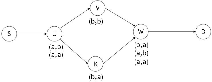
Example. Consider the path in the network illustrated by Fig. 3(a). The transition sequence corresponding to is and its trace is . The well-parenthesized sequence from is .
Let denotes the empty word, “” indicates the concatenation operation, and denotes the transition sequence obtained from a path as explained above. The following definitions give a formal characterization of the feasible paths.
Definition 1
A sequence from is valid if and only if , where is the formal language recursively defined by:
Definition 2
A path is a feasible path in from to if:
- 1.
is a path in ,
- 2.
The well-parenthesized sequence from is valid,
- 3.
For each :
- (a)
if and or then
- (b)
if and or then
- (c)
if and or then
- (a)
The language of valid sequences is known as the generalized Dyck language [17]. It is well-known that this language is context free but not regular. Thus, push-down automata are naturally adapted to model this problem.
Example. The multi-domain network illustrated by Fig. 3(a) has routers and two protocols labeled and . Adaptation function capabilities are indicated below each node. For example, the node can encapsulate the protocol in the protocol (function denoted by ) or can passively transmit the protocol (function denoted by ). In this multi-domain network, the only feasible path between and is and involves the encapsulation of the protocol in the protocol by the node , the passive transmission of the protocol by the node and the decapsulation of the protocol from by the node . (functions , and respectively).
Problem definition. As explained above, our goal is to find a feasible multi-domain path. Furthermore, we set as an objective function either the size of the sequence of adaptation functions or the size of the path in number of nodes. Hence, the problem we aim to solve can be defined as follows:
4 From the network model to a PDA
In this section, we address the conversion from a network to a PDA. Algorithm 1 takes as input a network and converts it to a PDA , where is the set of states of the PDA, the input alphabet, the stack alphabet, the transition relation, the start state, the initial stack symbol and the accepting state, is the empty string. The automaton from is obtained as follows:
- 1.
Create a state of the automaton for each and each , except for the source node for which a single state is created,
- 2.
The top of the stack is the last encapsulated protocol,
- 3.
If the current state is then the current protocol is ,
- 4.
The adaptation functions will be converted into transitions in the PDA. A transition is denoted where is the state of the PDA before the transition, is the input character, is the top of the stack before the transition (it is popped by the transition), is the sequence of symbols pushed to the stack, and is the state of the PDA after the transition. Thus if then is a passive transition, if then is a push of , and if then is a pop,
- 5.
A passive transition of a protocol across a node is modeled as a transition without push or pop between the state and the following state . It is denoted ,
- 6.
An encapsulation of a protocol in a protocol by a node is modeled as a push of the character in the stack between the state and the following state . It is denoted 11 1 Note that, even if , the transition has the form . Characters in are only used as input characters. Characters indexing states and pushed characters in the stack are their equivalent in . ,
- 7.
A decapsulation of from by a node is modeled as a pop of the protocol from the stack. It is denoted .
Complexity. Each node from the graph generates states, except the source node . A fictitious final state is added. Thus, the number of states is at worst so in . The worst case complexity of algorithm 1 is in . We assume that the network is connected, so . Since is a subset of , then and . Thus, the upper bound complexity is in , which is also an upper bound for the number of transitions.
Proposition 1
Considering a network , a source and a destination , the language recognized by is the set of traces of the feasible paths from to in .
Proof 1
Let a feasible path in a network and its trace leading to a valid sequence . We aim to demonstrate that: is recognized by and is a path in and There exists a feasible path corresponding to in if is recognized by the PDA . It is sufficient to show that is a feasible path in if and only if is recognized by (i.e the final state is reached and the stack is empty).
From we deduce the following path in defined as a sequence of transitions. This path begins with transitions: for each s.t. . Hence, transition belongs to this set. Then, the path in follows the order induced by , for each element in , we consider one or two transitions in as follows:
- 1.
if then
- (a)
if or consider the transition where ,
- (b)
if or consider the transition , where
- (a)
- 2.
else (i.e., if ) then consider the transition .
Note that, if then .
It is clear that this sequence of transitions is a path in recognizing the trace . Since is a well parenthesized word, if then the head of the stack when reaching state contains and when reaching state , the head of the stack is reduced to . Then, when reaching state , the stack is empty.
Conversely, we can show with a similar construction that any well recognized word on a path in induces one unique trace of feasible paths in from to . ∎
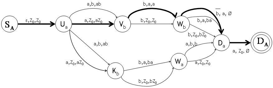
Example. Figure 3(b) is an example of output of algorithm 1. The algorithm transforms the network illustrated by Fig. 3(a) into a PDA of Fig 3(b). For instance, the link is transformed into the transitions and (pushes) because the node should encapsulate the protocol in the protocol using the adaptation function before transmitting to the node . The link is transformed into the transitions and (pushes) according to the adaptation function . It is also transformed into the transition (pop) because the node can decapsulate the protocol from using the adaptation function before transmitting to the node . The link is transformed into the transitions and (passive transitions) according the capability of the node (adaptation function ).
5 The shortest feasible path
In section 4, we provided a method to build a PDA allowing to determine the feasible paths. The next step is to minimize either the number of nodes or the number of adaptation functions. The method to minimize the number of nodes uses directly the PDA as described in section 5.1. But to minimize the number of adaptation functions, the PDA is transformed in order to bypass the sub-paths without any adaptation function, as detailed in section 5.2. Then, a CFG derived from the PDA (or the transformed PDA) generates words whose length is equivalent to the number of nodes (or to the number of adaptations). An algorithm browses the CFG to determine the shortest word. Finally, another algorithm identifies the multi-domain path corresponding to this shortest word.
5.1 Minimizing the number of nodes
The number of characters in a word accepted by the automaton is the number of links in the corresponding feasible path (each character is a protocol used on a link). Thus the step of automaton transformation (section 5.2) should be skipped. The automaton is directly transformed into a CFG, then the shortest word is generated as described in section 5.3.2. The corresponding feasible path is computed by algorithm 6 described in section 5.3.3.
5.2 Minimizing the number of adaptation functions
To enumerate only encapsulations and decapsulations in the length of each word (and thus minimize adaptation functions by finding the shortest word accepted), a transformed automaton in which all sequences involving passive transitions are bypassed must be determined. The length of the shortest word accepted by is the number of adaptation functions plus a fixed constant.
Let us define () as , and let be the sub-automaton induced by . By analogy with an induced subgraph, an induced sub-automaton is a multigraph with labeled edges such that the set of vertices is and the set of edges is the set of transitions between elements of . Since there are only passive transitions between two states in , all paths in the sub-automaton are passive. Let define as the shortest path length between and . This length can be computed between all pairs of nodes in using the Floyd-Warshall algorithm. Let be the set of successors of in the original automaton , i.e., .
Algorithm 2 takes as input and computes the transformed automaton . is initialized with the values of . Then, the algorithm computes the sub-automaton for each character (step (1)) and the length values for each pair of states in the sub-automaton (step (2)). Each path between a pair of states is a sequence of passive transitions. If such a path exists (step (3.1)), the algorithm adds transitions to from to each state in (steps (3.1.2) and (3.1.3)). These added transitions are the same that those which connect to its successors , but with an input character indexed by the number of passive transitions between and , (i.e., )) plus one (indicating that there is a transition sequence which matches with a sequence of protocols of length ). The indexed character is added to the input alphabet (step (3.1.1)).
Complexity. Computing the sub-automaton (step (1)) is done in by checking all the nodes and all the transitions. Computing the shortest path length between all pairs of states is done by the Floyd-Warshall algorithm in . If x=y, there are at worst transitions between and in (transitions in the form for all possible values of except — as the construction of the automaton forbids the encapsulation of a protocol in , and thus it is impossible to have as current protocol and at the top of the stack in the same time). If , there are at worst transitions between and in (the pop and the pushes for all possible values of except ). And as , the steps (3.1.2) and (3.1.3) are bounded by . However, a state belongs to only one sub-automaton, the complexity of algorithm 2 is therefore bounded by . And (see algorithm 1 for the construction of the set of states ). Thus, the complexity of algorithm 2 is in , which corresponds to in the network model. The number of transitions in is bounded by , which corresponds to in the network model.
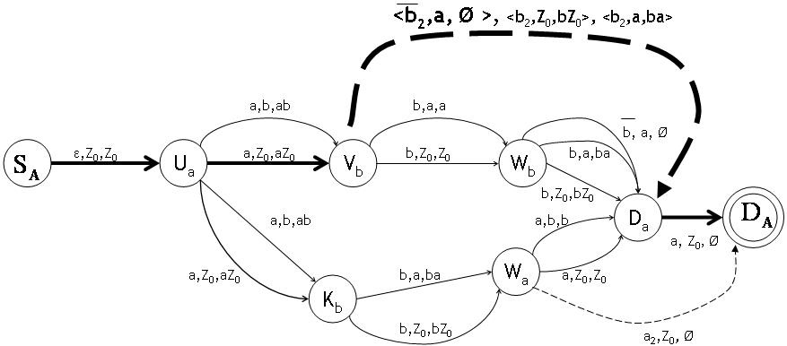
Example. Algorithm 2 transforms the PDA in Fig. 3(b) into the PDA in Fig. 3(c). For the protocol , the algorithm computes the sub-automaton induced by the states , and . The distance is then computed. Thus, to bypass the sequence of transitions , the transition is added.
Let be the set of words accepted by , and let be the set of words accepted by . Let be a function s.t.:
- 1.
if then
- 2.
if then
The domain of is extended to :
For simplicity, we consider that and are the same character. denotes the set of words accepted by transformed by (i.e. ).
It is clear that is not a bijection ()). So to operate the transformation between and , we define
for each , .
In other words, is the shortest word in s.t. .
The following lemmas and proposition show that the set of words accepted by the transformed automaton is ‘equivalent’ to the set of words accepted by the original automaton. Equivalent in the meaning that, using , each word accepted by the transformed automaton can be associated to a word accepted by the original one. In addition, the transformed automaton has a new propriety: there is a linear relation between the length of an accepted word and the minimum number of pushes (and pops) involved to accept it. This propriety allows to find the word requiring the minimum number of pushes accepted by the original automaton. This is done by finding the shortest word accepted by the transformed automaton.
Lemma 1
, the set of words accepted by and transformed by , is equal to , the set of words accepted by .
Proof 2
We prove this by double inclusion:
- 1.
(remind that we consider that ). So (1). On the other hand, the construction of by algorithm 2 does not delete any character, transition, state or set of final states from . So . And thus (2)
By (1) and (2), . - 2.
Let be a word in and let be a sequence of transitions accepting . For each transition () in this sequence, s.t. , there is a sequence of passive transitions in (because the creation of in requires the existence of such a sequence in ). This sequence begins from the state and is followed by a transition . Thus, this sequence in matches with And for each in , either so matches with (if ), or and there is a sequence of transitions in which matches with (if ). And since, by definition, , . Thus . ∎
Let be the shortest word accepted by , let be the minimum number of pushes in a sequence of transitions accepting in , and let be the minimum number of pops in a sequence of transitions accepting in .
Lemma 2
The length of the shortest path (sequence of transitions) accepting in is and .
Proof 3
First we prove that cannot be in the form of with . Let be the state in which is before reading the character . Let be the state in which is after reading and before reading . And let be the state in which is after reading . If , then, by construction, there is a transition (where is a pop of or a push of if ). So, if is replaced by in , the word obtained is shorter then and is also accepted by . Thus, the shortest word accepted by is where for .
By construction of , for each character in , there is a push transition if or a transition if . So all transitions in the shortest sequence that accepts are pops or pushes, except the first transition from the initial state and the final pop . The number of other pops is equal to the number of pushes (in order to have at the top of the stack before the final transition).∎
Now let be a word accepted by , let be the minimum number of pushes in a sequence of transitions accepting in , and let be the minimum number of pops in a sequence of transitions accepting in .
Lemma 3
For each :
- 1.
- 2.
Proof 4
Let be the sequence of transitions accepting in with minimum number of pushes and pops. For each sequence of passive transitions, followed by a push or a pop transition, there is a transition with the same push or pop and the same input character indexed by . So .
Let be the sequence of transitions with minimum pushes and pops accepting in . It is clear that . So if there is a sequence that accepts with less pops and pushes than , then each can be replaced by a sequence of passive transitions followed by a pop or a push in . And theses sequences accept (which is ) with less pops and pushes than in the sequence , which contradicts the fact that it minimizes the number of pops and pushes to accept . ∎
Proposition 2
The word accepted by which minimizes the number of pushes is , where is the shortest word (i.e., with minimum number of characters) accepted by .
Proof 5
By lemma 2, the shortest word accepted by minimizes the number of pushes in (since the number of pushes grows linearly as a function of the length of the word). Let be this word.
Suppose that there is a word accepted by such that . By lemma 3, , which leads to , while . Ad absurdum, is the word which minimizes the number of pushes in .∎
5.3 The shortest path as a shortest word
In order to find the shortest word accepted by (resp. ), the CFG such that (resp. ) is computed. The shortest word in is then generated.
5.3.1 From the PDA to the CFG.
The transformation of a PDA into a CFG is well-known. We adapted a general method described in [13] to transform (resp. ) into a CFG. The output of algorithm 3 is a CFG (resp. ) where is the set of nonterminals (variables), (resp. ) is the input alphabet, is the initial symbol (initial nonterminal) and is the set of production rules. Except , nonterminals are in the form where and (resp. and ). The demonstration of the correctness of this transformation is also in [13].
Complexity. The number of production rules in is bounded by (resp. . As all the nonterminals (except ) are in the form with and , the number of non terminals is bounded by (resp. ).
The worst case complexity of algorithm 3 is in (resp. ). W.r.t. the definition of the network, the upper bound is in (resp. ).
Example. This method transforms the PDA in Fig. 3(c) into a CFG. Figure 3(d) is a subset of production rules of the obtained CFG. This subset allows generating the shortest trace of a feasible path in the network in Fig. 3(a). For instance, the transition gives the production rule . The transition gives all the production rules where , including the production .
Remark. There are two mechanisms of acceptance defined for PDAs: an input word can be accepted either by empty stack (i.e., if the stack is empty after reading the word) or by final state (i.e., if a final state is reached after reading the word - even if the stack is not empty). Algorithm 3 takes as input an automaton which accepts words by empty stack. and accept words by empty stack and by final state, because the only transitions that empty the stack are those that reach the final state (the transitions in the form ). Thus, Algorithm 3 performs correctly with or as input.
5.3.2 The shortest word generated by a CFG.
To find the shortest word generated by , a function associates each nonterminal to the length of the shortest word that it generates.
More formally, s.t.:
- 1.
if then ,
- 2.
if then ,
- 3.
if (with ) then .
Algorithm 4 computes the value of for each .
Proposition 3
Algorithm 4 terminates at worst after iterations, and each obtained is the length (number of characters) of the shortest word produced by .
Proof 6
We prove that at each iteration (except the last one), there is a least one nonterminal s.t. is updated with the length of the shortest word that produces.Thus, the update of all with their correct values is done at worst in iterations. We proceed by induction on the number of iterations:
Basis: There is no -production in , and there is at least one production in the form where and (resp. ) (see algorithm 3 for the construction of ). For each . And algorithm 4 assigns these values to each at the first iteration.
Induction: Suppose that at iteration , there are at least nonterminals s.t. the algorithm has assigned the correct value to . So there are nonterminals which have not the correct -value yet.
- 1.
Either there is a nonterminal s.t. has not already the correct value (i.e., it can already be updated), but for all productions (each is a production) all nonterminals in have their correct -values. And thus, will be updated with the correct value at the end of the following iteration.
- 2.
Or, for each nonterminal with a wrong -value, there is at least a nonterminal in each of its productions which has not its correct -value yet.
- (a)
Either each contains a nonterminal which generates no word. Thus, generates no word and the value of is correct.
- (b)
Or all nonterminals in each generate a word. However, in the derivation of the shortest word generated by any nonterminal, no nonterminal is used twice or more (otherwise a shorter word can be generated by using this nonterminal once). Thus, among all nonterminals with a wrong -value, there is one which does not use others to generate its shortest word. So its -value is already correct or it will be updated to the correct value at the following iteration.∎
- (a)
Complexity. As there is at worst iteration of the while loop, the complexity of algorithm 4 is in which is (resp. ) in the network model
There are several algorithms which allow the generation of a uniform random word of some length from a CFG [12, 9, 18], or, more recently, a non-uniform random generation of a word according to some targeted distribution [5, 10]. For instance, the boustrophedonic and the sequential algorithms described in [9] generate a random labeled combinatorial object of some length from any decomposable structure (including CFGs). The boustrophedonic algorithm is in (where is the length of the object) and the sequential algorithm is in but may have a better average complexity. Both algorithms use a precomputed table of linear size. This table can be computed in . These algorithms require an unambiguous CFG, and the CFG computed by algorithm 3 can be inherently ambiguous depending on the input network (as several feasible paths can use the same sequence of protocols and thus have the same trace ). However, the unambiguity requirement is only for the randomness of the generation. Recall that our goal is to generate the trace of the shortest feasible path. Thus, we do not take into consideration the randomness and the distribution over the set of shortest traces. In order to generate the shortest word in , the boustrophedonic algorithm can take and as input (recall that is the length of the shortest word generated by ). Thus, the generation of the shortest word (resp. ) would have been in (resp. ), where denotes the length (number of characters) of . This complexity includes the precomputation of the table. However, this complexity hides factors depending of the size of the CFG, the construction of the precomputed table requires at least one pass over all the production rules.
Actually, as the -values are already computed, the generation can simply be done in linear time in the length of the shortest word. The standard algorithm 5 takes as input the CFG and the -values. Each nonterminal is replaced by the left part with minimal -value among its productions.
Complexity. Since there is no derivation of the form in (see algorithm 3), all branches in the derivation tree end with a character from (resp. ). The length of each branch is at worst (as a nonterminal does not appears twice in the same branch, otherwise a shorter word could be derivated by using this nonterminal once). Thus, the number of derivations and the complexity of algorithm 5 are bounded by (resp. ), which corresponds to (resp. ) in the network model.
5.3.3 From the shortest word to the path.
If the goal is to minimize the number of nodes in the path, algorithm 6 takes as input the shortest word accepted by . Otherwise, as is the shortest word accepted by and generated by , according to proposition 2, is the word which minimizes the number of pops and pushes in . In such a case it is the trace of the shortest feasible path in the network . It is possible that several paths match with the trace (resp. ). In such a case, a load-balancing policy can choose a path.
Algorithm 6 is a dynamic programming algorithm that computes . It starts at the node and takes at each step all the links in which match with the current character in . Let . At each step , the algorithm starts from each node in and adds to all links which match with . It also adds each in . When reaching , it backtracks to and selects the links from to .
Complexity. The loop stops exactly after steps, because it is sure that there is a feasible path of length if is accepted by the automaton . At each step, all links and nodes are checked in the worst case. Thus, algorithm 6 is in in the worst case.
6 Conclusion
| Algorithm | Upper-Bound Complexity | |
|---|---|---|
| Minimizing hops | Minimizing enc./dec. | |
| Algo. 1: Network to PDA | ||
| Algo. 2: Transform PDA | / | |
| Algo. 3: PDA to CFG | ||
| Algo. 4: Shortest word length | ||
| Algo. 5: Shortest word | ||
| Algo. 6: Shortest path | ||
The problem of path computation in a multi-layer network has been studied in the field of intra-domain path computation but is less addressed in the inter-domain field with consideration of the Pseudo-Wire architecture. There was no polynomial solution to this problem and the models used were not expressive enough to capture the encapsulation/decapsulation capabilities described in the Pseudo-Wire architecture.
In this paper, we provide algorithms that compute the shortest path in a multi-layer multi-domain network, minimizing the number of hops or the number of encapsulations and decapsulations. The presented algorithms involve Automata and Language Theory methods. A Push-Down Automaton models the multi-layer multi-domain network. It is then transformed in order to bypass passive transitions and converted into a Context-Free Grammar. The grammar generates the shortest protocol sequence, which allows to compute the path matching this sequence.
The different algorithms of our methodology have polynomial upper-bound complexity as summarized by Table 1. Compared to the preliminary version of this work, the proofs of correctness of the algorithms are detailed and the complexity analysis is significantly refined (the highest algorithm complexity is in instead of ).
In order to figure out the whole problem of end-to-end service delivery, we plan to extend our solution to support end-to-end Quality of Service constraints and model all technology constraints on the different layers (conversion or “mapping" of protocols). As a future work, we also plan to investigate which part of our algorithms can be distributed (e.g., Can the domains publish their encapsulation/decapsulation capabilities without disclosing their internal topology?) and how such a solution can be established on today’s architectures.

Acknowledgment
The first author would like to thank Kaveh Ghasemloo for his help about Algorithm 4. This work is partially supported by the ETICS-project, funded by the European Commission. Grant agreement no.: FP7-248567 Contract Number: INFSO-ICT-248567.
Appendix A List of notations
In order to facilitate the paper reading, Table 2 summarizes the symbols used in the paper.
| Symbols and their signification | Symbols and their signification |
|---|---|
| : The set of nodes of the network | : The set of links of the network |
| : The graph modeling the network topology | : The source node |
| : The destination node | : The alphabet (set of protocol) |
| : | P(U): The set of adaptation functions of node |
| : The set of all possible encapsulations and passive functions | : The set of all possible decapsulations |
| : The set of protocols that node can receive | : The set of protocols that node can send |
| : The set of protocols that can passively cross node | : Passive function |
| : Encapsulation of protocol in | : Decapsulation of protocol from |
| : The sequence of protocols used over the path (trace of ) | : Sequence of adaptation functions involved in path (transition sequence of ) |
| : The well-parenthesized sequence of | : Automaton corresponding to network |
| : The set of states of | : The input alphabet of |
| : The stack alphabet of | : The set of transitions of |
| : Initial state of | : Initial stack symbol |
| : Final state of | : A transition between states and , where is read, is popped from the stack and is pushed on the stack |
| : Sub-automaton indexed by | : Transformed PDA |
| : Language accepted by | : Minimum number of pushes in a sequence of transitions accepting the word in |
| : Context-free grammar corresponding to network | : The set of nonterminals of |
| : Initial nonterminal (axiom) of | : The set of production rules of |
| : Length of the shortest word generated by nonterminal |
References
- [1] M. Bocci and S. Bryant. RFC5659 - An Architecture for Multi-Segment Pseudowire Emulation Edge-to-Edge, 2009.
- [2] S. Bryant and P. Pate. RFC3985 - Pseudo Wire Emulation Edge-to-Edge (PWE3) Architecture, 2005.
- [3] I. Chlamtac, A. Faragó, and T. Zhang. Lightpath (Wavelength) Routing in Large WDM Networks. IEEE Journal on Selected Areas in Communications, 14(5):909–913, 1996.
- [4] H. Cho, J. Ryoo, and D. King. Stitching dynamically and statically provisioned segments to construct end-to-end multi-segment pseudowires. http://www.ietf.org/id/draft-cho-pwe3-mpls-tp-mixed-ms-pw-setup-01.txt, 2011.
- [5] A. Denise, Y. Ponty, and M. Termier. Controlled non-uniform random generation of decomposable structures. Theoretical Computer Science, 411(40-42):3527–3552, 2010.
- [6] F. Dijkstra, B. Andree, K. Koymans, J. van der Ham, P. Grosso, and C. de Laat. A multi-layer network model based on ITU-T G.805. Comput. Netw., 2008.
- [7] F. Dijkstra, J. Van der Ham, P. Grosso, and C. de Laat. A path finding implementation for multi-layer networks. Future Generation Comp. Syst., 25(2):142–146, 2009.
- [8] A. Farrel, JP. Vasseur, and J. Ash. RFC4655 - A Path Computation Element (PCE)-Based Architecture, 2006.
- [9] Ph. Flajolet, P. Zimmermann, and B. Van Cutsem. A calculus for the random generation of labelled combinatorial structures. Theoretical Computer Science, 1994.
- [10] D. Gardy and Y. Ponty. Weighted random generation of context-free languages: Analysis of collisions in random urn occupancy models. GASCom, 2010.
- [11] S. Gong and B. Jabbari. Optimal and Efficient End-to-End Path Computation in Multi-Layer Networks. In ICC, pages 5767–5771, 2008.
- [12] T. Hickey and J. Cohen. Uniform random generation of strings in a context-free language. SIAM J. Comput., 12(4):645–655, 1983.
- [13] J. E. Hopcroft, R. Motwani, and J. D. Ullman. From PDA’s to Grammars. In Introduction to Automata Theory, Languages, and Computation, chapter 6.3.2, pages 247–251. Addison-Wesley Longman Publishing Co., Inc., Boston, MA, USA, 2006.
- [14] F. A. Kuipers and F. Dijkstra. Path selection in multi-layer networks. Computer Communications, 2009.
- [15] M. L. Lamali, H. Pouyllau, and D. Barth. Path computation in Multi-Layer multi-domain networks. In IFIP/TC6 Networking 2012 (NETWORKING 2012), Prague, Czech Republic, May 2012.
- [16] M.L. Lamali, H. Pouyllau, and D. Barth. End-to-End Quality of Service in Pseudo-Wire Networks. In ACM CoNEXT Student Workshop, 2011.
- [17] Jens Liebehenschel. Lexicographical Generation of a Generalized Dyck Language. SIAM J. Comput., 2003.
- [18] H. G. Mairson. Generating Words in a Context-Free Language Uniformly at Random. Inf. Process. Lett., 49(2):95–99, 1994.
- [19] L. Martini, E. Rosen, N. El-Aawar, and G. Heron. RFC4448 - Encapsulation Methods for Transport of Ethernet over MPLS Networks, 2008.
- [20] K. Shiomoto, D. Papadimitriou, JL. Le Roux, M. Vigoureux, and D. Brungard. RFC5212 - Requirements for GMPLS-based multi-region and multi-layer networks (MRN/MLN), 2008.
- [21] Y(J). Stein, R. Shashoua, R. Insler, and M. Anavi. RFC5087 - Time Division Multiplexing over IP (TDMoIP), 2007.
- [22] W. Yao and B. Ramamurthy. A Link Bundled Auxiliary Graph Model for Constrained Dynamic Traffic Grooming in WDM Mesh Networks. IEEE Journal on Selected Areas in Communications, 23(8):1542–1555, 2005.
- [23] H. Zhu, H. Zang, K. Zhu, and B. Mukherjee. A novel generic graph model for traffic grooming in heterogeneous WDM mesh networks. IEEE/ACM Trans. Netw., 11(2):285–299, 2003.