In addition to the Higgs boson, $m_{h}=125.7(4)$ GeV [1], the experiments at LHC recently indicated a possibility for a resonance in the diphoton spectrum at about $750$ GeV [2]. While its spin must be either $J=0$ or $2$, its parity cannot be yet assessed. If, after improving statistics and further examining systematics of the data sample, this signal remains as such, a plausible explanations for the newly observed state could be the ones offered in refs. [3, 4, 5, 6, 7, 8, 9, 10, 11, 12, 13].

The simplest possibility is to consider scenarios with two Higgs doublets (2HDM) in which the spectrum of scalars consists of two CP-even ($h$ and $H$), one CP-odd ($A$) and one charged Higgs state ($H^{\pm}$). In this paper, we focus on the possibility of the new state being the CP-odd Higgs and find that the general theoretical constraints combined with the two known masses result in the bounds on the remaining two Higgs boson states. We also show that the resulting bounds and the proposed scenario satisfy the electroweak precision tests, and do not significantly modify the low energy (semi-)leptonic decay modes.

Let us stress that, in a pure 2HDM, the production cross section for the heavy spin-$0$ states seems to be too low to explain the claimed excess of $\sigma(gg\to X)B(X\to\gamma\gamma)$, where $X$ stands for the new $750$ GeV resonance, in such a way that an extended particle content might be needed [8]. However, our conclusions on the spectrum of the model are unlikely to be significantly affected by the additional particles as long as they are fermions. ¹¹ 1 In principle, our analysis of the electroweak precision tests would be affected by the presence of new fermions. However, the final outcome of such tests would be model dependent. One should be cautious and study carefully the signal strength, including the background contamination in the signal region as well as the possible signal-background interference, which in general are model dependent [14]. It should be reemphasized that other possibilities can be envisaged, such as the one in which $H$ and $A$ are mass degenerate. In this paper, we focus on the possibility of $A$ being the desired state hinted at about $750$ GeV.

The most general CP-conserving 2HDM potential compatible with gauge symmetries of the Standard Model is given by (see eg. ref. [15]),

	$\displaystyle V(\Phi_{1},\Phi_{2})=m_{11}^{2}\Phi_{1}^{\dagger}\Phi_{1}$	$\displaystyle+m_{22}^{2}\Phi_{2}^{\dagger}\Phi_{2}-m_{12}^{2}(\Phi_{1}^{\dagger}\Phi_{2}+\Phi_{2}^{\dagger}\Phi_{1})+\dfrac{\lambda_{1}}{2}(\Phi_{1}^{\dagger}\Phi_{1})^{2}+\dfrac{\lambda_{2}}{2}(\Phi_{2}^{\dagger}\Phi_{2})^{2}$		(1)
		$\displaystyle+\lambda_{3}\Phi_{1}^{\dagger}\Phi_{1}\Phi_{2}^{\dagger}\Phi_{2}+\lambda_{4}\Phi_{1}^{\dagger}\Phi_{2}\Phi_{2}^{\dagger}\Phi_{1}+\dfrac{\lambda_{5}}{2}\left[(\Phi_{1}^{\dagger}\Phi_{2})^{2}+(\Phi_{2}^{\dagger}\Phi_{1})^{2}\right],$

where $\Phi_{1}$ and $\Phi_{2}$ are the two complex scalar $SU(2)$ doublets with hypercharge $Y=+1$. In the above expression the $\mathcal{Z}_{2}$ symmetry ($\Phi_{1,2}\to-\Phi_{1,2}$) has been tacitly assumed, except for the soft symmetry breaking term proportional to $m_{12}^{2}$. Assuming that each doublet carries a non-zero vacuum expectation value (vev) one can write,

$$\Phi_{a}=\begin{pmatrix}\phi_{a}^{+}\\ \frac{1}{\sqrt{2}}(v_{a}+\rho_{a}+i\eta_{a})\end{pmatrix},\qquad a=1,2,$$

(2)

with both vev’s $v_{1,2}$ being associated with the neutral components to avoid a problem of breaking the $U(1)$ symmetry of electromagnetism. A further assumption is the conservation of CP-symmetry in the Higgs sector which translates to $v_{1,2}\in\mathbb{R}$. Two of the six fields ($\phi_{1,2}^{+}$, $\rho_{1,2}$, $\eta_{1,2}$) are Goldstone bosons and can be gauged away, which then leaves us with the physical spectrum consisting of one charged $H^{\pm}$, two CP-even neutral $h,H$, and one CP-odd neutral $A$ boson, that are linear combinations of the above fields, namely,

		$\displaystyle H^{+}=\phi_{1}^{+}\sin\beta-\phi_{2}^{+}\cos\beta,$	$\displaystyle A=\eta_{1}\sin\beta-\eta_{2}\cos\beta,$
		$\displaystyle H=-\rho_{1}\cos\alpha-\rho_{2}\sin\alpha,$	$\displaystyle h=\rho_{1}\sin\alpha-\rho_{2}\cos\alpha,$		(3)

with $\alpha$ and $\beta$ associated with rotations that diagonalize the mass matrices. Written in terms of parameters given in $V(\Phi_{1},\Phi_{2})$ one gets,

$$\tan\beta=\dfrac{v_{2}}{v_{1}},\qquad\tan(2\alpha)=\dfrac{2(-m_{12}^{2}+\lambda_{345}v_{1}v_{2})}{m_{12}^{2}(v_{2}/v_{1}-v_{1}/v_{2})+\lambda_{1}v_{1}^{2}-\lambda_{2}v_{2}^{2}},$$

(4)

where $\lambda_{345}\equiv\lambda_{3}+\lambda_{4}+\lambda_{5}$. After setting $\sqrt{v_{1}^{2}+v_{2}^{2}}\equiv v^{\rm SM}=246.2$ GeV (which in the following will be referred to as $v$), $\tan\beta$ becomes the free model parameter and the quartic couplings $\lambda_{1-5}$ can be expressed in terms of scalar masses and mixing angles as [16]:

	$\displaystyle\lambda_{1}$	$\displaystyle=\frac{1}{v^{2}}\left(-\tan^{2}\beta M^{2}+\frac{\sin^{2}\alpha}{\cos^{2}\beta}m_{h}^{2}+\frac{\cos^{2}\alpha}{\cos^{2}\beta}m_{H}^{2}\right),$		(5)
	$\displaystyle\lambda_{2}$	$\displaystyle=\frac{1}{v^{2}}\left(-\cot^{2}\beta M^{2}+\frac{\cos^{2}\alpha}{\sin^{2}\beta}m_{h}^{2}+\frac{\sin^{2}\alpha}{\sin^{2}\beta}m_{H}^{2}\right),$		(6)
	$\displaystyle\lambda_{3}$	$\displaystyle=\frac{1}{v^{2}}\left(-M^{2}+2m_{H^{\pm}}^{2}+\dfrac{\sin 2\alpha}{\sin 2\beta}(m_{H}^{2}-m_{h}^{2})\right),$		(7)
	$\displaystyle\lambda_{4}$	$\displaystyle=\frac{1}{v^{2}}\left(M^{2}+m_{A}^{2}-2m_{H^{\pm}}^{2}\right)$		(8)
	$\displaystyle\lambda_{5}$	$\displaystyle=\frac{1}{v^{2}}\left(M^{2}-m_{A}^{2}\right),$		(9)

in an obvious notation in which we also replaced $M^{2}\equiv\dfrac{m_{12}^{2}}{\sin\beta\cos\beta}$. Conversely,

	$\displaystyle m_{H}^{2}$	$\displaystyle=M^{2}\sin^{2}(\alpha-\beta)+\left(\lambda_{1}\cos^{2}\alpha\cos^{2}\beta+\lambda_{2}\sin^{2}\alpha\sin^{2}\beta+\frac{\lambda_{345}}{2}\sin 2\alpha\sin 2\beta\right)v^{2},$		(10)
	$\displaystyle m_{h}^{2}$	$\displaystyle=M^{2}\cos^{2}(\alpha-\beta)+\left(\lambda_{1}\sin^{2}\alpha\cos^{2}\beta+\lambda_{2}\cos^{2}\alpha\sin^{2}\beta-\frac{\lambda_{345}}{2}\sin 2\alpha\sin 2\beta\right)v^{2},$		(11)
	$\displaystyle m_{A}^{2}$	$\displaystyle=M^{2}-\lambda_{5}v^{2},$		(12)
	$\displaystyle m_{H^{\pm}}^{2}$	$\displaystyle=M^{2}-\frac{\lambda_{45}}{2}v^{2}.$		(13)

To ensure that the scalar potential is bounded from below, the quartic parameters in Eq. (1) should satisfy [17]

$$\lambda_{1,2}>0,\qquad{}\lambda_{3}>-(\lambda_{1}\lambda_{2})^{1/2},\qquad{}\text{and}\qquad{}\lambda_{3}+\lambda_{4}-|\lambda_{5}|>-(\lambda_{1}\lambda_{2})^{1/2}.$$

(14)

Stability of the vacuum ($\partial V/\partial v_{1,2}=0$) amounts to solving

	$\displaystyle m_{11}^{2}+\dfrac{\lambda_{1}v_{1}^{2}}{2}+\dfrac{\lambda_{3}v_{2}^{2}}{2}=\dfrac{v_{2}}{v_{1}}\left[m_{12}^{2}-(\lambda_{4}+\lambda_{5})\dfrac{v_{1}v_{2}}{2}\right],$		(15)
	$\displaystyle m_{22}^{2}+\dfrac{\lambda_{2}v_{2}^{2}}{2}+\dfrac{\lambda_{3}v_{1}^{2}}{2}=\dfrac{v_{1}}{v_{2}}\left[m_{12}^{2}-(\lambda_{4}+\lambda_{5})\dfrac{v_{1}v_{2}}{2}\right],$		(16)

which cannot be done analytically for $m_{12}\neq 0$. Instead, one can derive a condition that is necessary and sufficient for $V(\Phi_{1},\Phi_{2})$ to have a global minimum at $(v_{1},v_{2})$ and it reads [18],

$$m_{12}^{2}\left(m_{11}^{2}-m_{22}^{2}\sqrt{\lambda_{1}/\lambda_{2}}\right)\left(\tan\beta-\sqrt[4]{\lambda_{1}/\lambda_{2}}\right)>0\,.$$

(17)

Another generic constraint comes from the requirement of unitarity of the $S$-wave component of the partial wave decomposition of the full Higgs scattering amplitudes. That condition can be translated into a set of constraints on the quartic couplings in Eq. (1), which amounts to [19]

$$|a_{\pm}|,|b_{\pm}|,|c_{\pm}|,|f_{\pm}|,|e_{1,2}|,|f_{1}|,|p_{1}|<8\pi,$$

(18)

where

	$\displaystyle a_{\pm}$	$\displaystyle=\frac{3}{2}(\lambda_{1}+\lambda_{2})\pm\sqrt{\frac{9}{4}(\lambda_{1}-\lambda_{2})^{2}+(2\lambda_{3}+\lambda_{4})^{2}},$		(19)
	$\displaystyle b_{\pm}$	$\displaystyle=\frac{1}{2}(\lambda_{1}+\lambda_{2})\pm\frac{1}{2}\sqrt{(\lambda_{1}-\lambda_{2})^{2}+4\lambda_{4}^{2}},$		(20)
	$\displaystyle c_{\pm}$	$\displaystyle=\frac{1}{2}(\lambda_{1}+\lambda_{2})\pm\frac{1}{2}\sqrt{(\lambda_{1}-\lambda_{2})^{2}+4\lambda_{5}^{2}},$		(21)
	$\displaystyle e_{1}$	$\displaystyle=\lambda_{3}+2\lambda_{4}-3\lambda_{5},\qquad\qquad\qquad e_{2}=\lambda_{3}-\lambda_{5},$		(22)
	$\displaystyle f_{+}$	$\displaystyle=\lambda_{3}+2\lambda_{4}+3\lambda_{5},\qquad\qquad\qquad f_{-}=\lambda_{3}+\lambda_{5},$		(23)
	$\displaystyle f_{1}$	$\displaystyle=\lambda_{3}+\lambda_{4},\qquad\qquad\qquad\qquad\quad p_{1}=\lambda_{3}-\lambda_{4}.$		(24)

We then generate random points in the parameter space by fixing $m_{h}=125.7(4)\,\rm{GeV}$, $v=246.22\,\rm{GeV}$, as well as $m_{A}=750(30)$ GeV, and by varying

	$\displaystyle\tan\beta\in[1,35]\,,\qquad\quad\alpha\in[-\frac{\pi}{2},\frac{\pi}{2}]\,,\qquad m_{H}\in(m_{h},1.5\,\mathrm{TeV}]$
	$\displaystyle m_{H^{\pm}}\in(m_{W},1.5\,\mathrm{TeV}]\,,\quad|M^{2}|={|m_{12}^{2}|\over\sin\beta\cos\beta}<(1.5\,\rm{TeV})^{2}\,,$		(25)

to select those that are consistent with constraints given in Eqs.(14–18).

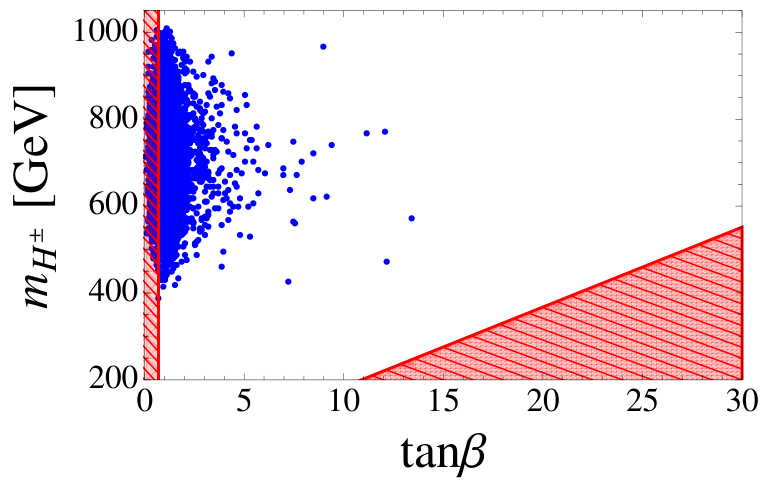
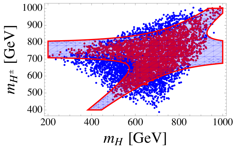
Two interesting results of our scan are shown in Fig. 1 where we see that the lower values of $\tan\beta$ are highly favored with most of the points being $\tan\beta\lesssim 5$, and that the mass of the other two Higgs states are bounded both from below and from above, namely,

$\displaystyle 400\ {\rm GeV}\lesssim m_{H^{\pm}}\lesssim 1~{\rm TeV},\qquad 200\ {\rm GeV}\lesssim m_{H}\lesssim 1~{\rm TeV}.$

(26)

Furthermore we observe that the $Z_{2}$-symmetry breaking term cannot be excessively large and it reproduces $m_{A}=750(30)$ GeV, for $|M|\in(200,800)$ GeV. Finally the resulting points are concentrated in the region of $|\cos(\beta-\alpha)|\lesssim 0.3$, which then means that the couplings $g_{hVV}>g_{HVV}$ for $V$ being either $W$ or $Z$. ²² 2 We remind the reader that $g_{HVV}=2\cos(\beta-\alpha)m_{V}^{2}/v$ and $g_{hVV}=2\sin(\beta-\alpha)m_{V}^{2}/v$. This result agrees with the findings of ref. [20].

Another interesting feature is that one cannot impose the degeneracy $m_{h}=m_{H}$ and scan over the parameter space as indicated above (but without fixing $m_{A}$). While most of $\tan\beta$ points remain small, the values of $\cos(\alpha-\beta)$ are equidistributed between $-1$ and $1$, but one then gets an upper bound on $m_{A}\lesssim 700$ GeV, inconsistent with the state supposedly observed at LHC. We should also mention that the direct experimental searches of the non-Standard Model Higgs states also restrict $\cos(\alpha-\beta)$ to small values, as recently discussed in Refs. [21, 22].

As it is well known, in order to avoid the tree level flavor changing neutral currents (FCNC), one imposes that the fermions of definite charge and chirality couple to a specific Higgs doublet. In this way one distinguishes various types of 2HDM: In Type I models all fermions couple to the same Higgs doublet ($\Phi_{2}$, by convention); In Type II the right-handed (RH) quarks with charge ${\cal Q}=2/3$ couple to the doublet $\Phi_{2}$, whereas those with ${\cal Q}=-1/3$ to the doublet $\Phi_{1}$. A slight modification of the latter rule leads to two other types: Type X 2HDM (or lepton-specific), and type Z (or flipped) one. Their coupling patterns to quarks and leptons are listed in Tab. 1. More general, in terms of Yukawa couplings, is the so called Type III 2HDM in which the couplings to fermions are all to be fixed by the data [23] which is often impractical because of too many free parameters so that one has to resort to additional assumptions such as minimal flavor violation (MFV) [24, 25], the natural flavor conservation [26], or the aligned 2HDM [27] where the minimal flavor violation is ensured by assuming proportionality between the matrices of Yukawa couplings to the two Higgs doublets.

The Yukawa interaction Lagrangian for the neutral currents can be written as [15],

$\displaystyle\mathcal{L}_{\mathrm{Y}}^{nc}$

$\displaystyle=-\sum_{f={u,d,\ell}}\frac{m_{f}}{v}\left(C_{hf}\ \bar{f}fh+C_{Hf}\ \bar{f}fH-iC_{Af}\ \bar{f}\gamma_{5}fA\right),$

(27)

where the sum runs over up- and down-type quarks, as well as leptons. Here we focus on the coupling $C_{Af}$ which depends on $\tan\beta$ and is given for various types of 2HDM in Tab. 2.

With this in mind, the expression for the decay width of the CP-odd Higgs to two fermions reads,

$\displaystyle\Gamma(A\to f\bar{f})={N_{c}\over 8\pi}|C_{Af}|^{2}{m_{f}^{2}\over v^{2}}\sqrt{m_{A}^{2}-4m_{f}^{2}}\,$

(28)

where $N_{c}=3$ for quarks, and $1$ otherwise. Quite obviously the full width $\Gamma(A)$ will be highly dominated by the top quark. As for the decay to two photons, one has [28],

$\displaystyle\Gamma(A\to\gamma\gamma)={\alpha^{2}m_{A}^{3}\over 64v^{2}\pi^{3}}\left|\sum_{f}N_{c}Q_{f}^{2}C_{Af}F\left({m_{A}^{2}\over 4m_{f}^{2}}\right)\right|^{2},$

(29)

where the triangle loop induces the factor,

$\displaystyle F(x)=\left\{\begin{array}[]{ll}\displaystyle\frac{1}{x}\arcsin^{2}\sqrt{x}&x\leq 1\\ \displaystyle-\frac{1}{4x}\left[\log\frac{1+\sqrt{1-x^{-1}}}{1-\sqrt{1-x^{-1}}}-i\pi\right]^{2}&x>1\,.\end{array}\right.$

The expression for the decay width of $A\to Z\gamma$ reads [29],

$\displaystyle\Gamma(A\to Z\gamma)={\alpha^{2}m_{A}^{3}N_{c}\over 384v^{2}\pi^{3}}C_{At}^{2}\left({1-(8/3)\sin^{2}\theta_{w}\over\sin\theta_{w}\cos\theta_{w}}\right)^{2}\left(1-\frac{m_{Z}^{2}}{m_{A}^{2}}\right)^{3},$

(33)

and its contribution to the full decay width is smaller than the other modes discussed above.

In Fig. 2 we plot the partial decay width for $A\to t\bar{t}$, $A\to b\bar{b}$, $A\to\tau\tau$, $A\to\gamma\gamma$ and $A\to Z\gamma$ for all four types of the 2HDM discussed here. As expected, the $A\to t\bar{t}$ mode is largely dominant and essentially saturates the width of the CP-odd Higgs boson, $\Gamma(A)$, the results of which are given in Tab. 3 for four different values of $\tan\beta$. Since the experimenters are searching for the $A\to\tau\tau$ mode, in the same table we also give the values of $B(A\to\tau\tau)$ for all four types of 2HDM considered here. It is worth emphasizing that for small values of $\tan\beta$ the width $\Gamma(A)$ is quite large and can accommodate the observation made by ATLAS, namely that the better fits are obtained for the new resonance having a width $\sim 40$ GeV. Similar conclusion holds true for the $H$ boson, the coupling of which to $t\bar{t}$ is proportional to $1/\tan\beta$ for small $\cos(\beta-\alpha)$.

Finally, with the above ingredients we can also compute the dominant decay channel $H^{\pm}\to tb$, the decay width of which is given by,

$\displaystyle\Gamma(H^{\pm}\to tb)={1\over 8\pi}{|V_{tb}|^{2}\over v^{2}}\left(C_{Ab}^{2}m_{b}^{2}+C_{At}^{2}m_{t}^{2}-4C_{At}C_{Ab}{m_{b}^{2}m_{t}^{2}\over m_{H^{\pm}}^{2}-m_{t}^{2}}\right){(m_{H^{\pm}}^{2}-m_{t}^{2})^{2}\over m_{H^{\pm}}^{3}},$

(34)

while for the leptonic decay we have

$\displaystyle\Gamma(H^{\pm}\to\ell\bar{\nu}_{\ell})={m_{H^{\pm}}\over 8\pi}\left({C_{A\ell}m_{\ell}\over v}\right)^{2}.$

(35)

The results for the branching fraction $B(H^{\pm}\to\tau\nu_{\tau})$ are given in Tab. 3. Before concluding this Section we would like to emphasise once again that the bounds on the Higgs states are derived by considering the general theoretical arguments. The most significant bound comes from the tree-level unitarity constraints (18), and the effects of heavy fermions (beyond the Standard Model) would enter only through loops and are therefore unlikely to significantly alter the statements we made about the Higgs states.

As it is well known, the additional scalar states present in a 2HDM contribute to the gauge bosons vacuum polarizations, and are as such constrained by electroweak precision data. The scalar contributions to the Peskin-Takeuchi parameters $S$, $T$, and $U$ for the 2HDM case can be found e.g. in ref. [30]. In order to compute the related bounds on the spectrum, we used the latest Gfitter values for the best fit, uncertainties and covariance matrix [31],

$$\begin{aligned} &\Delta S^{SM}=0.05\pm 0.11,\\ &\Delta T^{SM}=0.09\pm 0.13,\\ &\Delta U^{SM}=0.01\pm 0.11,\\ \end{aligned}\qquad\qquad V=\left(\begin{array}[]{ccc}1&0.90&-0.59\\ 0.90&1&-0.83\\ -0.59&-0.83&1\end{array}\right),$$

(36)

composing the $\chi^{2}$ function as

$$\chi^{2}=\sum_{i,j}(X_{i}-X_{i}^{\rm SM})(\sigma^{2})_{ij}^{-1}(X_{j}-X_{j}^{\rm SM}),$$

(37)

with $X_{i}=\Delta S,\Delta T,\Delta U$ and the covariance matrix $\sigma^{2}_{ij}\equiv\sigma_{i}V_{ij}\sigma_{j}$, in which $(\sigma_{1},\sigma_{2},\sigma_{3})=(0.11,0.13,0.11)$.

In Fig. 3 we show the region allowed at 99% CL by electroweak precision data in the plane $m_{H}$ versus $m_{H^{\pm}}$. Since the coupling between the additional scalars and the gauge bosons depend on $\cos(\beta-\alpha)$ (see footnote 2), we present two representative cases: $\cos(\beta-\alpha)=0$ and $\cos(\beta-\alpha)=0.3,$ which according to Sec. 2, are the minimum and maximum value allowed by our scan. Note that most of the points which were previously allowed, Fig. 1, are still not excluded. Let us stress that, as already pointed out in the introduction, additional states which may be needed to increase the production cross section $\sigma(gg\to A)$ may affect significantly Fig. 3, but in a model dependent way. The analysis of the electroweak precision measurements in these extended models must be done case by case, and is beyond the scope of the paper.

Since the charged Higgs boson is now fully bounded [cf. Eq.(26)], the contribution from the charged Higgs can modify the low energy decay rates of the leptonic and semileptonic processes which generally agree with the Standard Model predictions within the error bars. To that end we add a term involving the couplings to the scalar sector to the effective Hamiltonian of the Standard Model at low energies, namely

$\displaystyle\mathcal{H}_{\text{eff}}=\sqrt{2}G_{F}V_{ud}$

$\displaystyle\Big[(\overline{u}\gamma_{\mu}d)(\overline{\ell}_{L}\gamma^{\mu}\nu_{L})+g_{S}(\mu)(\overline{u}d)(\overline{\ell}_{R}\nu_{L})+g_{P}(\mu)(\overline{u}\gamma^{5}d)(\overline{\ell}_{R}\gamma^{5}\nu_{L})\Big]+\text{h.c.},$

(38)

where $u$ and $d$ stand for the generic up- and down-type quark flavor. Using this Hamiltonian one can easily compute the semileptonic and the leptonic decay rates for the specific channels, e.g. $B\to D\tau\nu_{\tau}$ and $B\to\tau\nu_{\tau}$, and we obtain

		$\displaystyle{dB\over dq^{2}}(B\to D\tau\nu_{\tau})={\tau_{B}G_{F}^{2}\over 192\pi^{3}m_{B}^{3}}|V_{cb}|^{2}|f_{+}(q^{2})|^{2}\left[c_{+}(q^{2})+c_{0}(q^{2})\left(1+g_{S}{q^{2}\over m_{\tau}(m_{b}-m_{c})}\right)^{2}\left|{f_{0}(q^{2})\over f_{+}(q^{2})}\right|^{2}\right],$		(39)
		$\displaystyle B(B\to\tau\nu_{\tau})=\tau_{B}{G_{F}^{2}m_{B}m_{\tau}^{2}\over 8\pi}|V_{ub}|^{2}f_{B}^{2}\left(1-\frac{m_{\tau}^{2}}{m_{B}^{2}}\right)^{2}\left(1-g_{P}{m_{B}^{2}\over m_{\tau}m_{b}}\right)^{2},$		(40)

with $\tau_{B}$ being the $B$-meson lifetime, $m_{\tau}^{2}\leq q^{2}\leq(m_{B}-m_{D})^{2}$,

		$\displaystyle c_{+}(q^{2})=\lambda^{3/2}(q^{2})q^{2}\left[1-\frac{3}{2}{m_{\tau}^{2}\over q^{2}}+\frac{1}{2}\left({m_{\tau}^{2}\over q^{2}}\right)^{3}\right],$		(41)
		$\displaystyle c_{0}(q^{2})=\lambda^{1/2}(q^{2})m_{\tau}^{2}\frac{3}{2}{m_{B}^{4}\over q^{2}}\left(1-{m_{\tau}^{2}\over q^{2}}\right)^{2}\left(1-{m_{D}^{2}\over m_{B}^{2}}\right)^{2},$		(42)

and $\lambda(q^{2})=[q^{2}-(m_{B}+m_{D})^{2}][q^{2}-(m_{B}-m_{D})^{2}]$. The decay constant ($f_{B}$) and the form factors [$f_{+,0}(q^{2})$] are defined via,

	$\displaystyle\langle 0|\bar{u}\gamma_{\mu}\gamma_{5}b|B(p)\rangle=if_{B}p_{\mu}\,,$		(43)
	$\displaystyle\langle D(p^{\prime})|\bar{c}\gamma_{\mu}b|B(p)\rangle=\left(p_{\mu}+p^{\prime}_{\mu}-{m_{B}^{2}-m_{D}^{2}\over q^{2}}q_{\mu}\right)f_{+}(q^{2})+{m_{B}^{2}-m_{D}^{2}\over q^{2}}q_{\mu}f_{0}(q^{2})\,.$		(44)

Notice that we consider the pseudoscalar to pseudoscalar meson decay for which the decay form factors are better controlled through numerical simulations of QCD on the lattice [32]. As it can be seen from the above expressions, for $g_{S,P}\neq 0$ the helicity suppression is lifted and the contribution coming from coupling to the charged scalar could be important. The explicit expressions for $g_{S,P}$, in terms of the quark and lepton masses as well as $m_{H^{\pm}}$ and $\tan\beta$, in various types of 2HDM read:

Type	$g_{S}$	$g_{P}$
I	$-\dfrac{m_{\ell}}{{m^{2}_{H^{\pm}}}}(m_{d}-m_{u})\cot^{2}\beta$	$\dfrac{m_{\ell}}{{m^{2}_{H^{\pm}}}}(m_{d}+m_{u})\cot^{2}\beta$
II	$-\dfrac{m_{\ell}}{{m^{2}_{H^{\pm}}}}(m_{u}+m_{d}\tan^{2}\beta)$	$-\dfrac{m_{\ell}}{{m^{2}_{H^{\pm}}}}(m_{u}-m_{d}\tan^{2}\beta)$
$X$	$\dfrac{m_{\ell}}{{m^{2}_{H^{\pm}}}}(m_{d}-m_{u})$	$-\dfrac{m_{\tau}}{{m^{2}_{H^{\pm}}}}(m_{d}+m_{u})$
$Z$	$\dfrac{m_{\ell}}{{m^{2}_{H^{\pm}}}}(m_{d}+m_{u}\cot^{2}\beta)$	$-\dfrac{m_{\ell}}{{m^{2}_{H^{\pm}}}}(m_{d}-m_{u}\cot^{2}\beta)$

By averaging the values obtained by BaBar [33] and Belle [34], we have $B(B\to\tau\nu_{\tau})=1.44(32)\times 10^{-4}$, which we then combine with $f_{B}=188(6)$ MeV [32], and $V_{ub}=3.6(1)\times 10^{-3}$ as obtained from the global fit by UTfit and CKM-fitter [35], to conclude that for all types of 2HDM considered here the resulting value for $B(B\to\tau\nu_{\tau})_{\rm 2HDM}$ is consistent with experiment and is practically indistinguishable from the Standard Model predictions. Only for large values of $\tan\beta\gtrsim 20$ the $B(B\to\tau\nu_{\tau})_{\rm 2HDM}$ may differ considerably from $B(B\to\tau\nu_{\tau})_{\rm SM}$ if the Type II 2HDM is adopted. That situation, however, is not of interest for our purpose since our scan does not allow $\tan\beta>15$. A plot of the resulting $B(B\to\tau\nu_{\tau})_{\rm 2HDM}$ as a function of $\tan\beta$ is shown in Fig. 4 for the extreme values of charged Higgs boson, $m_{H^{\pm}}=400$ GeV and $m_{H^{\pm}}=1$ TeV, and compared to the experimental value at $2\sigma$-level.

In the case of $B(D_{s}\to\tau\nu_{\tau})_{\rm 2HDM}$ all type of 2HDM remain perfectly consistent with the Standard Model prediction which agrees with the experimentally established $B(D_{s}\to\tau\nu_{\tau})=5.54(24)\times 10^{-2}$ [1].

As for the semileptonic decay, we consider the ratio $R_{D}=B(B\to D\tau\nu_{\tau})/B(B\to D\mu\nu_{\mu})$ in which a significant part of theoretical uncertainties cancel. Its value has been measured in three experiments [36, 37, 38] leading to an average of $R_{D}=0.41(5)$. That result is consistent with the SM value, $R_{D}^{\rm SM}=0.31(2)$ [39], at less than $2\sigma$-level and also with the 2HDM scenarios discussed here. Like in the case of leptonic decay, only in the Type II model at moderately large values of $\tan\beta$ one can see a small deviation with respect to the Standard Model, as shown in Fig. 4. That deviation is however too small to be probed experimentally for $\tan\beta<15$. As for the loop induced processes, one extra constraint can be obtained from the comparison between the experimentally established ${B}(B_{s}\to\mu^{+}\mu^{-})_{\mathrm{exp}}=\left(2.8^{+0.7}_{-0.6}\right)\times 10^{-9}$ [40] with the Standard Model prediction [41] leading to

$\displaystyle{R}_{s\mu}\equiv\dfrac{B(B_{s}\to\mu^{+}\mu^{-})}{B(B_{s}\to\mu^{+}\mu^{-})_{\mathrm{SM}}},\quad{\rm and}\quad{R}_{s\mu}^{\text{exp}}=0.76^{+0.20}_{-0.18}\,.$

(45)

Using, instead of the Standard Model, the expressions for Wilson coefficients computed in a generic 2HDM [42] leads to the exclusion bound on the very low $\tan\beta\lesssim 0.7$, as shown in Fig. 4.

In this paper we showed that the CP-odd Higgs is a plausible candidate for the resonance observed by both the CMS and the ATLAS experiments at LHC in the diphoton spectrum around $750$ GeV. From the general considerations in the framework of 2HDM, and after fixing $m_{h}=125.7(4)$ GeV and $m_{A}=750(30)$ GeV, we find the upper and lower bounds to the masses of the remaining two Higgs bosons, namely

$\displaystyle 400\ {\rm GeV}\lesssim m_{H^{\pm}}\lesssim 1~{\rm TeV},\qquad 200\ {\rm GeV}\lesssim m_{H}\lesssim 1~{\rm TeV}.$

(46)

From our scan, in which we used the general constraints spelled out in Eqs. (14–18), we also find that the preferred values of $\tan\beta$ are relatively small, $\tan\beta<15$, with most of the points concentrated in the region $\tan\beta<5$. The width of the CP-odd Higgs is dominated by the $A\to t\bar{t}$ mode and its value significantly depends on $\tan\beta$. We find that the width can be large [as large as $\Gamma(A)\simeq 40$ GeV, for $\tan\beta=1$]. Furthermore, we find that $|\cos(\beta-\alpha)|\lesssim 0.3$, i.e. not far from the Standard Model, and in agreement with the results of the SFitter analysis [20], and with the direct searches [21, 22].

We then checked that for the range of $\tan\beta$ and $m_{H^{\pm}}$ obtained from our scan, the semileptonic and leptonic decay modes are not significantly modified with respect to the Standard Model predictions. We also checked that the spectrum of the 2HDM considered here is fully consistent with electroweak precision data encoded in the $S$, $T$, $U$ parameters.

The plots, in which all the constraints considered in this paper are included, are presented in Fig. 5. Notice in particular that $B(B\to\tau\nu_{\tau})$ and $R_{D}$ provide very similar bounds in the $(\tan\beta,m_{H^{\pm}})$ plane for $m_{H^{\pm}}\in(0.4,1)$ TeV. They, at best, exclude the large values of $\tan\beta$ in the Type II model, otherwise they are insensitive to the parameter space (small $\tan\beta$) we are considering here. $B(B_{s}\to\mu^{+}\mu^{-})$, instead, provides an important constraint, i.e. exclusion of the very small values of $\tan\beta$. Since that last constraint involves coupling to the top-quark, it is independent of the type of the 2HDM.

Finally, we need to stress once again that our ambition was not to provide a full scenario of physics beyond the Standard Model. Rather, we merely attempt whether or not the recent experimental hint of the excess at LHC can be consistent with the interpretation of the CP-odd Higgs in the general framework of 2HDM. We find that scenario plausible and the repercussions on the remaining Higgs bosons look quite appealing because they can be either confirmed or refuted experimentally quite soon. Since the announcement of the LHC results [2] many authors discussed $\sigma(gg\to X)B(X\to\gamma\gamma)$, where $X$ stands for the resonance we claim to be consistent with the CP-odd Higgs, being larger than expected in the 2HDM alone. At this point one should be careful about interpretation of such results because: (a) they are not published or publicly announced, and (b) a careful study of the signal strength and of the signal-background interference, including the appropriate cuts, is mandatory. The conclusion we reached here is solely based on considerations of the spectrum of scalars and it cannot be significantly changed in the presence of additional fermionic degrees of freedom, assuming the mixing between the Standard Model fermions and the extra heavy fermions is indeed small.

This work was partially supported by Fundação de Amparo à Pesquisa do Estado de São Paulo (FAPESP) and Conselho Nacional de Ciência e Tecnologia (CNPq). D.B. acknowledges the INP-CNRS support via“Inphyniti”.

References

- [1] K. A. Olive et al. [Particle Data Group Collaboration], Chin. Phys. C 38 (2014) 090001.
- [2] LHC seminar “ATLAS and CMS physics results from Run 2”, talks by Jim Olsen and Marumi Kado, CERN, 15 Dec. 2015.; ATLAS note, ATLAS-CONF-2015-081; CMS note, CMS PAS EXO-15-004.
- [3] R. Franceschini et al., arXiv:1512.04933 [hep-ph].
- [4] K. Harigaya and Y. Nomura, arXiv:1512.04850 [hep-ph]; Y. Nakai, R. Sato and K. Tobioka, arXiv:1512.04924 [hep-ph].
- [5] T. Higaki, K. S. Jeong, N. Kitajima and F. Takahashi, arXiv:1512.05295 [hep-ph];
- [6] D. Buttazzo, A. Greljo and D. Marzocca, arXiv:1512.04929 [hep-ph]; S. D. McDermott, P. Meade and H. Ramani, arXiv:1512.05326 [hep-ph].
- [7] J. Ellis, S. A. R. Ellis, J. Quevillon, V. Sanz and T. You, arXiv:1512.05327 [hep-ph].
- [8] A. Angelescu, A. Djouadi and G. Moreau, arXiv:1512.04921 [hep-ph]; M. Low, A. Tesi and L. T. Wang, arXiv:1512.05328 [hep-ph].
- [9] B. Bellazzini, R. Franceschini, F. Sala and J. Serra, arXiv:1512.05330 [hep-ph]; C. Petersson and R. Torre, arXiv:1512.05333 [hep-ph].
- [10] S. Di Chiara, L. Marzola and M. Raidal, arXiv:1512.04939 [hep-ph]; R. S. Gupta, S. Jäger, Y. Kats, G. Perez and E. Stamou, arXiv:1512.05332 [hep-ph].
- [11] S. Knapen, T. Melia, M. Papucci and K. Zurek, arXiv:1512.04928 [hep-ph].
- [12] Y. Mambrini, G. Arcadi and A. Djouadi, arXiv:1512.04913 [hep-ph]; M. Backovic, A. Mariotti and D. Redigolo, arXiv:1512.04917 [hep-ph].
- [13] P. S. Bhupal Dev and A. Pilaftsis, JHEP 1412 (2014) 024 [JHEP 1511 (2015) 147] [arXiv:1408.3405 [hep-ph]].
- [14] N. Greiner, S. Liebler and G. Weiglein, arXiv:1512.07232 [hep-ph].
- [15] G. C. Branco, P. M. Ferreira, L. Lavoura, M. N. Rebelo, M. Sher and J. P. Silva, Phys. Rept. 516 (2012) 1 [arXiv:1106.0034 [hep-ph]].
- [16] S. Kanemura, Y. Okada, E. Senaha and C.-P. Yuan, Phys. Rev. D 70 (2004) 115002 [hep-ph/0408364].
- [17] J. F. Gunion and H. E. Haber, Phys. Rev. D 67 (2003) 075019 [hep-ph/0207010].
- [18] A. Barroso, P. M. Ferreira, I. P. Ivanov and R. Santos, JHEP 1306 (2013) 045 [arXiv:1303.5098 [hep-ph]].
- [19] S. Kanemura, T. Kubota and E. Takasugi, Phys. Lett. B 313 (1993) 155 [hep-ph/9303263]; B. Swiezewska, Phys. Rev. D 88 (2013) 5, 055027 [ibid 88 (2013) 11, 119903] [arXiv:1209.5725 [hep-ph]].
- [20] T. Corbett, O. J. P. Eboli, D. Goncalves, J. Gonzalez-Fraile, T. Plehn and M. Rauch, JHEP 1508 (2015) 156 [arXiv:1505.05516 [hep-ph]].
- [21] L. Brenner, “Constraints on new phenomena through Higgs coupling measurements with the ATLAS detector”, talk presented at the International Conference on Supersymmetry and Unification of Fundamental Interactions, SUSY 2015, c.f https://indico.cern.ch/event/331032/session/7/contribution/237
- [22] G. Aad et al. [ATLAS Collaboration], JHEP 1503 (2015) 088 [arXiv:1412.6663 [hep-ex]]; Phys. Rev. D 92 (2015) 5, 052002 [arXiv:1505.01609 [hep-ex]]; arXiv:1512.03704 [hep-ex]; V. Khachatryan et al. [CMS Collaboration], JHEP 1511 (2015) 018 [arXiv:1508.07774 [hep-ex]]; CMS Collaboration [CMS Collaboration], CMS-PAS-HIG-14-029; P. Onyisi [ATLAS and CMS Collaborations], PoS FPCP 2015 (2015) 023.
- [23] A. Crivellin, A. Kokulu and C. Greub, Phys. Rev. D 87 (2013) 9, 094031 [arXiv:1303.5877 [hep-ph]]; ibid 86 (2012) 054014 [arXiv:1206.2634 [hep-ph]]; F. Mahmoudi and O. Stal, Phys. Rev. D 81 (2010) 035016 [arXiv:0907.1791 [hep-ph]].
- [24] G. D’Ambrosio, G. F. Giudice, G. Isidori and A. Strumia, Nucl. Phys. B 645 (2002) 155 [hep-ph/0207036]; G. Blankenburg and G. Isidori, Eur. Phys. J. Plus 127 (2012) 85 [arXiv:1107.1216 [hep-ph]]; E. Nikolidakis and C. Smith, Phys. Rev. D 77 (2008) 015021 [arXiv:0710.3129 [hep-ph]].
- [25] A. Celis, V. Ilisie and A. Pich, JHEP 1307 (2013) 053 [arXiv:1302.4022 [hep-ph]]; W. Altmannshofer, S. Gori and G. D. Kribs, Phys. Rev. D 86 (2012) 115009 [arXiv:1210.2465 [hep-ph]].
- [26] A. J. Buras, M. V. Carlucci, S. Gori and G. Isidori, JHEP 1010 (2010) 009 [arXiv:1005.5310 [hep-ph]].
- [27] M. Jung, A. Pich and P. Tuzon, JHEP 1011 (2010) 003 [arXiv:1006.0470 [hep-ph]]; A. Pich and P. Tuzon, Phys. Rev. D 80 (2009) 091702 [arXiv:0908.1554 [hep-ph]].
- [28] M. Spira, A. Djouadi, D. Graudenz and P. M. Zerwas, Nucl. Phys. B 453 (1995) 17 [hep-ph/9504378].
- [29] J. F. Gunion, H. E. Haber and C. Kao, Phys. Rev. D 46 (1992) 2907.
- [30] R. Barbieri, L. J. Hall, Y. Nomura and V. S. Rychkov, Phys. Rev. D 75 (2007) 035007 [hep-ph/0607332].
- [31] M. Baak et al. [Gfitter Group Collaboration], Eur. Phys. J. C 74 (2014) 3046 [arXiv:1407.3792 [hep-ph]].
- [32] S. Aoki et al., Eur. Phys. J. C 74 (2014) 2890 [arXiv:1310.8555 [hep-lat]].
- [33] J. P. Lees et al. [BaBar Collaboration], Phys. Rev. D 88 (2013) 3, 031102 [arXiv:1207.0698 [hep-ex]].
- [34] B. Kronenbitter et al. [Belle Collaboration], Phys. Rev. D 92 (2015) 5, 051102 [arXiv:1503.05613 [hep-ex]].
- [35] J. Charles et al., Phys. Rev. D 91 (2015) 7, 073007 [arXiv:1501.05013 [hep-ph]]; M. Bona et al. [UTfit Collaboration], Phys. Lett. B 687 (2010) 61 [arXiv:0908.3470 [hep-ph]].
- [36] J. P. Lees et al. [BaBar Collaboration], Phys. Rev. D 88 (2013) 7, 072012 [arXiv:1303.0571 [hep-ex]].
- [37] M. Huschle et al. [Belle Collaboration], Phys. Rev. D 92 (2015) 7, 072014 [arXiv:1507.03233 [hep-ex]].
- [38] G. Ciezarek [LHCb Collaboration], talk presented at Flavor Physics & CP violation 2015 (Nagoya, Japan, 25-29 May 2015), [fpcp2015.hepl.phys.nagoya-u.ac.jp].
- [39] D. Becirevic, N. Kosnik and A. Tayduganov, Phys. Lett. B 716 (2012) 208 [arXiv:1206.4977 [hep-ph]]; J. A. Bailey et al. [MILC Collaboration], Phys. Rev. D 92 (2015) 3, 034506 [arXiv:1503.07237 [hep-lat]]; H. Na et al. [HPQCD Collaboration], Phys. Rev. D 92 (2015) 5, 054510 [arXiv:1505.03925 [hep-lat]]; M. Atoui, V. Morenas, D. Becirevic and F. Sanfilippo, Eur. Phys. J. C 74 (2014) 5, 2861 [arXiv:1310.5238 [hep-lat]].
- [40] V. Khachatryan et al. [CMS and LHCb Collaborations], Nature 522 (2015) 68 [arXiv:1411.4413 [hep-ex]].
- [41] C. Bobeth, M. Gorbahn, T. Hermann, M. Misiak, E. Stamou and M. Steinhauser, Phys. Rev. Lett. 112 (2014) 101801 [arXiv:1311.0903 [hep-ph]].
- [42] X. Q. Li, J. Lu and A. Pich, JHEP 1406 (2014) 022 [arXiv:1404.5865 [hep-ph]].