Composite Models for the 750 GeV Diphoton Excess

Preprint: UCB-PTH-15/15

Keisuke Harigaya and Yasunori Nomura Affiliation: Berkeley Center for Theoretical Physics, Department of Physics, University of California, Berkeley, CA 94720 Affiliation: Theoretical Physics Group, Lawrence Berkeley National Laboratory, Berkeley, CA 94720

Abstract

We present composite models explaining the diphoton excess of mass around $750~{\rm GeV}$ recently reported by the LHC experiments.

I Introduction

Recently, the existence of a diphoton excess of mass around $750~{\rm GeV}$ has been reported by both the ATLAS [1] and CMS [2] experiments at the LHC. The signals are still only $3.6~\sigma$ and $2.6~\sigma$ in the respective experiments, but if confirmed, this would indicate the long awaited discovery of new physics at the TeV scale.

Because of the Landau-Yang theorem [3], a particle decaying into two photons must have either spin 0, 2, or higher. Assuming spin 0, it is natural to postulate that the particle is a composite state of some strong dynamics around the TeV scale, since it would then not introduce any new hierarchy problem beyond that of the standard model Higgs boson, which may have an environmental understanding [4].

In fact, the relevance of strong dynamics is also suggested by the data. Suppose the diphoton resonance is a scalar field $S$ of mass $m_{S}\simeq 750~{\rm GeV}$ , whose couplings to the gluon and photon are induced by the following interaction

{\cal L}=\lambda SQ\bar{Q},

(1)

where $\lambda$ is a coupling constant, and $(Q,\bar{Q})$ is a heavy vector-like fermion of mass $m_{Q}$ charged under the standard model gauge group, $SU(3)_{C}\times SU(2)_{L}\times U(1)_{Y}$ . Assuming that $(Q,\bar{Q})$ is an $SU(3)_{C}$ triplet and has charge $q$ , its loop generates

{\cal L}\sim\frac{1}{24\pi^{2}}\frac{\lambda S}{m_{Q}}\biggl(\frac{1}{2}g_{3}^{2}G^{a\mu\nu}G^{a}_{\mu\nu}+3(qe)^{2}F^{\mu\nu}F_{\mu\nu}\biggr),

(2)

where $g_{3}$ and $e$ are the QCD and QED gauge couplings, respectively, and $G^{a}_{\mu\nu}$ and $F_{\mu\nu}$ are the corresponding field strengths. The production cross section of $S$ through gluon fusion times the branching ratio into diphoton is then given by

\sigma_{pp\rightarrow S}B_{S\rightarrow AA}\simeq 0.2~{\rm fb}\times\lambda^{2}\left(\frac{q}{2/3}\right)^{4}\left(\frac{600~{\rm GeV}}{m_{Q}}\right)^{2}.

(3)

Here, we have normalized $m_{Q}$ by its experimental lower bound [5]. (Note also that the decay of $S$ into $Q\bar{Q}$ must be kinematically forbidden in order not to suppress the diphoton signal, giving $m_{Q}>m_{S}/2\simeq 375~{\rm GeV}$ .) We find that to reproduce the observed excess, which requires $\sigma_{pp\rightarrow S}B_{S\rightarrow AA}\sim 10~{\rm fb}$ , the coupling $\lambda$ must be rather large. This suggests the existence of strong dynamics behind the physics generating couplings between the resonance of interest and standard model gauge bosons.

Motivated by these considerations, in this paper we present models in which the observed diphoton excess arises from a composite particle of some hidden strong gauge interactions. We present a scenario in which the particle is a state around the dynamical scale (a hidden glueball or a hidden eta prime) as well as a scenario in which it is lighter (a hidden pion). We see that some of the models have possible tensions with diboson searches at $8~{\rm TeV}$ , but others do not. In particular, we find that the model having the charge assignment consistent with $SU(5)$ grand unification has a parameter region in which the observed diphoton excess is reproduced without contradicting the other data. In general, the models described here yield multiple resonances in the TeV region, which may be observed in the future LHC data.

In the appendix, we present a general analysis of constraints from the $8~{\rm TeV}$ data in the case that the scalar resonance is coupled to the standard model gauge fields only through dimension-5 operators.

II Hidden Glueball: Minimal Model

Consider a hidden gauge group $G_{H}$ , with the dynamical scale (the mass scale of generic resonances) $\Lambda$ . For simplicity, we take $G_{H}$ to be $SU(N)$ . We also introduce a vector-like hidden quark $(Q,\bar{Q})$ of mass $m$ , whose charges under $G_{H}$ and the standard model $SU(3)_{C}$ and $U(1)_{Y}$ are given in Table 1. Here, $Q$ and $\bar{Q}$ represent left-handed Weyl spinors.

	$G_{H}$	$SU(3)_{C}$	$U(1)_{Y}$
$Q$	$\Box$	$\bar{\Box}$	$a$
$\bar{Q}$	$\bar{\Box}$	$\Box$	$-a$

Table 1: Charge assignment of a hidden “heavy” quark. Here,

a\neq 0

, and

Q

and

\bar{Q}

are left-handed Weyl spinors.

For $m\gtrsim\Lambda$ , the hidden quark can be regarded as a “heavy” quark (with respect to $\Lambda$ ), and the lightest hidden hadron will be a glueball $s$ consisting of hidden sector gauge fields, of mass

m_{s}\sim\Lambda.

(4)

Due to the existence of $(Q,\bar{Q})$ , we expect that this state couples to the standard model gauge fields as

{\cal L}\sim-\frac{\Lambda^{3}}{4\pi m^{4}}s\left(\frac{g_{3}^{2}}{2}G^{a\mu\nu}G^{a}_{\mu\nu}+\frac{9a^{2}g_{1}^{2}}{5}B^{\mu\nu}B_{\mu\nu}\right),

(5)

where $a=1,\cdots,8$ is the $SU(3)_{C}$ adjoint index, and $g_{3}$ and $g_{1}$ are the $SU(3)_{C}$ and $U(1)_{Y}$ gauge couplings, respectively.¹¹ 1 Throughout the paper, we adopt the hypercharge normalization such that the standard model fermions have $(q,\bar{u},\bar{d},l,\bar{e})=(1/6,-2/3,1/3,-1/2,1)$ , and $g_{1}$ is in the $SU(5)$ normalization. Here and below, we count possible factors of $4\pi$ using naive dimensional analysis [6].

The hidden glueball state $s$ can be produced by gluon fusion (among others) and decay into diphoton with the branching ratio

B_{s\rightarrow\gamma\gamma}=\frac{81a^{4}}{50}\frac{\cos^{4}\theta_{W}g_{1}^{4}}{8g_{3}^{4}}\simeq 0.033\,a^{4},

(6)

where $\theta_{W}$ is the Weinberg angle. The production cross section of $s$ through Eq. (5) at $13~{\rm TeV}$ $pp$ collisions can be estimated (after multiplying the diphoton branching ratio) as

\sigma_{pp\rightarrow s}B_{s\rightarrow\gamma\gamma}\sim 10~{\rm fb}\times a^{4}\left(\frac{3.5~{\rm TeV}}{m^{4}/\Lambda^{3}}\right)^{2},

(7)

where we have used NNPDF 3.0 [7] for the parton distribution function. We thus find that

\Lambda\sim 700~{\rm GeV},\qquad m\sim 1~{\rm TeV},

(8)

give $m_{s}$ and $\sigma_{pp\rightarrow s}B_{s\rightarrow\gamma\gamma}$ roughly consistent with the excess in the $13~{\rm TeV}$ data.

The model is subject to constraints from analogous high-mass diboson resonance searches in the $8~{\rm TeV}$ data. Assuming that the production occurs through interactions in Eq. (5), the ratio of the $s$ production cross sections at $8~{\rm TeV}$ and $13~{\rm TeV}$ is

\frac{\sigma_{pp\rightarrow s}|_{\rm 8\,TeV}}{\sigma_{pp\rightarrow s}|_{\rm 13\,TeV}}\simeq 0.21,

(9)

for $m_{s}=750~{\rm GeV}$ . This gives $\sigma_{pp\rightarrow s}B_{s\rightarrow\gamma\gamma}$ close to the upper limit from the $8~{\rm TeV}$ data [8]. The model also gives definite predictions for the relative branching ratios between $s\rightarrow\gamma\gamma,ZZ$ , and $Z\gamma$

	$\displaystyle\frac{B_{s\rightarrow ZZ}}{B_{s\rightarrow\gamma\gamma}}$	$\displaystyle=\tan^{4}\theta_{W}\simeq 0.09,$		(10)
	$\displaystyle\frac{B_{s\rightarrow Z\gamma}}{B_{s\rightarrow\gamma\gamma}}$	$\displaystyle=2\tan^{2}\theta_{W}\simeq 0.6,$		(11)

where we have ignored the phase space factors. With Eq. (9), we thus obtain

\sigma\times B|_{Z\gamma,\,{\rm 8\,TeV}}\simeq 1.3~{\rm fb}\left(\frac{\sigma\times B|_{\gamma\gamma,\,{\rm 13\,TeV}}}{10~{\rm fb}}\right).

(12)

This is consistent with the upper limit from the $8~{\rm TeV}$ data [9].

We note that the precise value of $\sigma\times B|_{{\rm 8\,TeV}}$ depends on the details of $s$ production, which we have assumed here to occur only through Eq. (5). (For an analysis of constraints from the $8~{\rm TeV}$ data for general dimension-5 couplings between $s$ and the standard model gauge fields, see the appendix.) The assumption of gluon fusion dominated production, however, may not be valid in some cases. For example, depending on the values of $m$ and $\Lambda$ , production of heavy resonances that are composed of $Q$ and $\bar{Q}$ and decay into $s$ may give comparable contributions to the production of single $s$ through the gluon fusion. With this production mechanism, the production rates of $s$ in $8~{\rm TeV}$ and $13~{\rm TeV}$ $pp$ collisions will differ more, relaxing the constraints from the $8~{\rm TeV}$ data. The production mechanisms can be differentiated experimentally, e.g., through the transverse momentum distribution of photons. Detailed analyses of this issue are warranted.

Limits from other diboson decays of $s$ , i.e. to $gg$ and $ZZ$ , are weaker.

III Hidden Pion: Minimal Model

We now consider a model in which the $750~{\rm GeV}$ resonance is a hidden “pion,” instead of the hidden glueball. A virtue of this model is that we need to rely less on the dynamical assumption about the hidden sector. As before, we take the hidden gauge group $G_{H}$ to be $SU(N)$ , but now we take the hidden quarks to have charges in Table 2 and mass terms

{\cal L}=-m_{1}Q_{1}\bar{Q}_{1}-m_{2}Q_{2}\bar{Q}_{2}+{\rm h.c.},

(13)

where we take $m_{1,2}>0$ without loss of generality.

	$G_{H}$	$SU(3)_{C}$	$U(1)_{Y}$	$U(1)_{A}$
$Q_{1}$	$\Box$	$\bar{\Box}$	$a$	$1/3$
$Q_{2}$	$\Box$	${\bf 1}$	$b$	$-1$
$\bar{Q}_{1}$	$\bar{\Box}$	$\Box$	$-a$	$1/3$
$\bar{Q}_{2}$	$\bar{\Box}$	${\bf 1}$	$-b$	$-1$

Table 2: Charge assignment of hidden “light” quarks. Here,

a^{2}\neq b^{2}

, and

Q_{1,2}

and

\bar{Q}_{1,2}

are left-handed Weyl spinors.

We assume that these masses are sufficiently smaller than the dynamical scale, $m_{1,2}\ll\Lambda$ , so that $Q_{1,2}$ and $\bar{Q}_{1,2}$ can be regarded as hidden “light” quarks.

III.1 Hidden Pion Dynamics

The strong $G_{H}$ dynamics makes the hidden quarks condensate

\langle Q_{1}\bar{Q}_{1}\rangle\approx\langle Q_{2}\bar{Q}_{2}\rangle\equiv\langle Q\bar{Q}\rangle\approx\frac{1}{16\pi^{2}}\Lambda^{3}.

(14)

These condensations do not break the standard model $SU(3)_{C}$ or $U(1)_{Y}$ , since the hidden quark quantum numbers under these gauge groups are vector-like with respect to $G_{H}$ [10]. The spectrum below $\Lambda$ then consists of hidden pions, arising from spontaneous breaking of approximate $SU(4)_{A}$ axial flavor symmetry:

\begin{array}[]{ll}\psi\sim Q_{1}\bar{Q}_{1}&({\bf Adj},0),\\ \chi\sim Q_{1}\bar{Q}_{2}&(\Box,a-b),\\ \phi\sim Q_{1}\bar{Q}_{1}-Q_{2}\bar{Q}_{2}&({\bf 1},0),\end{array}

(15)

where $\psi$ and $\phi$ are real scalars while $\chi$ is a complex scalar. The quantum numbers in the rightmost column represent those under $SU(3)_{C}\times U(1)_{Y}$ . The masses of these particles are given by [11]

$\displaystyle m_{\psi}^{2}$	$\displaystyle=2m_{1}\frac{\langle Q\bar{Q}\rangle}{f^{2}}+3\Delta_{C},$	(16)
$\displaystyle m_{\chi}^{2}$	$\displaystyle=(m_{1}+m_{2})\frac{\langle Q\bar{Q}\rangle}{f^{2}}+\frac{4}{3}\Delta_{C}+\frac{3(a-b)^{2}}{5}\Delta_{Y},$	(17)
$\displaystyle m_{\phi}^{2}$	$\displaystyle=\frac{m_{1}+3m_{2}}{2}\frac{\langle Q\bar{Q}\rangle}{f^{2}}.$	(18)

Here, $f$ is the decay constant, given by

f\approx\frac{1}{4\pi}\Lambda,

(19)

and $\Delta_{C}$ and $\Delta_{Y}$ are contributions from $SU(3)_{C}$ and $U(1)_{Y}$ gauge loops, of order

\Delta_{C}\approx\frac{g_{3}^{2}}{16\pi^{2}}\Lambda^{2},\qquad\Delta_{Y}\approx\frac{g_{1}^{2}}{16\pi^{2}}\Lambda^{2}.

(20)

We assume that $\phi$ is the lightest hidden pion, which can be ensured by making $m_{2}$ smaller with respect to $m_{1}$ . This particle is the pseudo Nambu-Goldstone boson of $U(1)_{A}\subset SU(4)_{A}$ , whose charges are given in Table 2. The couplings of $\phi$ to the standard model gauge fields are determined by the $U(1)_{A}$ - $SU(3)_{C}^{2}$ and $U(1)_{A}$ - $U(1)_{Y}^{2}$ anomalies and are given by²² 2 The definition of our decay constant, $f$ , is a factor of $2$ smaller than that in Ref. [11]: $f=F/2$ .

{\cal L}=-\frac{Ng_{3}^{2}}{32\sqrt{6}\pi^{2}f}\phi G^{a\mu\nu}\tilde{G}^{a}_{\mu\nu}-\frac{9(a^{2}-b^{2})Ng_{1}^{2}}{80\sqrt{6}\pi^{2}f}\phi B^{\mu\nu}\tilde{B}_{\mu\nu},

(21)

where $\tilde{G}^{a}_{\mu\nu}\equiv\epsilon_{\mu\nu\rho\sigma}G^{a\rho\sigma}/2$ and similarly for $\tilde{B}_{\mu\nu}$ . Therefore, $\phi$ can be produced by gluon fusion and decay into diphoton with a significant branching ratio. Similar anomaly induced couplings also exist between $\psi$ and $G^{\mu\nu}\tilde{G}_{\mu\nu}$ and for $a\neq 0$ between $\psi$ and $G^{\mu\nu}\tilde{B}_{\mu\nu}=B^{\mu\nu}\tilde{G}_{\mu\nu}$ , but not for other combinations of hidden pions and standard model gauge bosons.

III.2 Parameter Region and Constraints

Assuming that $\phi$ production occurs only through interactions in Eq. (21), the production cross section at $13~{\rm TeV}$ $pp$ collisions is given by

\sigma_{pp\rightarrow\phi}\simeq 270~{\rm fb}\left(\frac{N}{5}\frac{600~{\rm GeV}}{f}\right)^{2}.

(22)

From Eq. (21), we find that

B_{\phi\rightarrow\gamma\gamma}=\frac{81(a^{2}-b^{2})^{2}\cos^{4}\theta_{W}g_{1}^{4}}{50g_{3}^{4}},

(23)

so we obtain

\sigma_{pp\rightarrow\phi}B_{\phi\rightarrow\gamma\gamma}\simeq 8.9~{\rm fb}\left(\frac{N(a^{2}-b^{2})}{5}\frac{600~{\rm GeV}}{f}\right)^{2}.

(24)

This determines the decay constant as

f\simeq 570~{\rm GeV}\,\frac{N(a^{2}-b^{2})}{5}\sqrt{\frac{10~{\rm fb}}{\sigma_{pp\rightarrow\phi}B_{\phi\rightarrow\gamma\gamma}}}.

(25)

We then obtain from Eq. (18, 19)

\frac{m_{1}+3m_{2}}{4}\approx\frac{m_{\phi}^{2}}{8\pi f}\simeq 40~{\rm GeV}\left(\frac{570~{\rm GeV}}{f}\right),

(26)

where we have used $m_{\phi}=750~{\rm GeV}$ in the last expression. Note, however, that this equation has an $O(1)$ uncertainty arising from an unknown coefficient in Eq. (19).

We thus find that the model reproduces the observed diphoton excess for

f\sim 600~{\rm GeV},\qquad m_{1,2}\sim 40~{\rm GeV}.

(27)

Since the relative branching ratios between $\phi\rightarrow\gamma\gamma,ZZ$ , and $Z\gamma$ are the same as those of $s$ in the previous model, Eqs. (10, 11), the present model is subject to the same constraints from searches of high-mass diboson resonances in the $8~{\rm TeV}$ data.

Other constraints on the model may come from the existence of heavier hidden pions, $\psi$ and $\chi$ . In particular, without higher dimension operators coupling the hidden and standard model sectors and suppressed by a scale not far above $\Lambda$ , the $\chi$ particle is stable at collider timescales. Once produced, it hadronizes picking up a light quark of the standard model. For $|a-b|=2/3$ and $1/3$ , for example, this particle appears as heavy stable top and bottom scalar quarks, respectively. The lower bounds on the masses of such particles are about $800\mbox{--}900~{\rm GeV}$ [12]. We expect that $m_{\chi}$ satisfies this bound for $m_{1}\sim m_{2}$ due to the contribution from $SU(3)_{C}$ gauge loop, $\Delta_{C}$ , but if not, we can always make $m_{\chi}>900~{\rm GeV}$ keeping $m_{\phi}=750~{\rm GeV}$ by making $m_{2}$ smaller relative to $m_{1}$ .

III.3 Variations—Hidden Eta Prime

It is interesting to consider a parameter region of the model with $m_{2}\ll\Lambda\ll m_{1}$ . In this case, we expect that the lightest hidden hadron is the hidden $\eta^{\prime}$ particle of mass $\sim\Lambda$ , consisting of $Q_{2}\bar{Q}_{2}$ . The production of this particle occurs through that of heavy resonances involving $Q_{1}$ and $\bar{Q}_{1}$ , which then decay into two or more hidden $\eta^{\prime}$ . (The decay of the lightest heavy resonance into an even number of $\eta^{\prime}$ would require parity violation, which can be provided by the $\theta$ term of $G_{H}$ , $\theta_{H}\neq 0$ .) This makes the production cross sections at $8~{\rm TeV}$ and $13~{\rm TeV}$ more hierarchical than in Eq. (9), alleviating/eliminating possible tensions with the $8~{\rm TeV}$ data. The decay of the hidden $\eta^{\prime}$ is mostly into two electroweak gauge bosons, without having a significant branching into two gluons.

We mention that this model may exhibit an intriguing set of signals if $\theta_{H}=0$ . In this case, a heavy “ $\eta$ ” consisting of $Q_{1}\bar{Q}_{1}$ , which we call $\tilde{\eta}$ , cannot decay into $\eta^{\prime}$ because of parity conservation (unless the three $\eta^{\prime}$ mode is kinematically open) and hence decays into $gg$ and $\gamma\gamma$ . On the other hand, a heavy “ $\rho$ ,” having $J^{PC}=1^{--}$ , decays into $\gamma$ and $\eta^{\prime}$ , which subsequently decays as $\eta^{\prime}\rightarrow\gamma\gamma$ . Therefore, by choosing $m_{\eta^{\prime}}=750~{\rm GeV}$ and $m_{\tilde{\eta}}\simeq 1.6~{\rm TeV}$ we may also be able to accommodate the second, (much) weaker diphoton excess seen around $1.6~{\rm TeV}$ in the ATLAS data [1]. To be conclusive, however, a more detailed analysis is needed.

IV Models Consistent with Unification

We finally discuss a model in which the charge assignment of the hidden quarks is consistent with $SU(5)$ grand unification [13]. We take the hidden quarks to be a vector-like fermion in the bifundamental representation of $G_{H}$ and $SU(5)$ , as shown in Table 3, and write down their mass terms as in Eq. (13). Depending on the relative sizes of $\Lambda$ and $m_{1,2}$ , this model realizes either the hidden glueball or hidden pion scenario.

	$G_{H}$	$SU(3)_{C}$	$SU(2)_{L}$	$U(1)_{Y}$	$U(1)_{A}$
$Q_{1}$	$\Box$	$\bar{\Box}$	${\bf 1}$	$1/3$	$1/3$
$Q_{2}$	$\Box$	${\bf 1}$	$\Box$	$-1/2$	$-1/2$
$\bar{Q}_{1}$	$\bar{\Box}$	$\Box$	${\bf 1}$	$-1/3$	$1/3$
$\bar{Q}_{2}$	$\bar{\Box}$	${\bf 1}$	$\Box$	$1/2$	$-1/2$

Table 3: Charge assignment of hidden quarks consistent with grand unification.

IV.1 Hidden Glueball

For $m_{1,2}\gtrsim\Lambda$ , the lightest hidden hadron is the hidden glueball $s$ , which interacts with the standard model gauge fields as

	$\displaystyle{\cal L}\sim$	$\displaystyle-\frac{\Lambda^{3}}{4\pi m_{1}^{4}}s\left(\frac{g_{3}^{2}}{2}G^{a\mu\nu}G^{a}_{\mu\nu}+\frac{g_{1}^{2}}{5}B^{\mu\nu}B_{\mu\nu}\right)$
		$\displaystyle-\frac{\Lambda^{3}}{4\pi m_{2}^{4}}s\left(\frac{g_{2}^{2}}{2}W^{b\mu\nu}W^{b}_{\mu\nu}+\frac{3g_{1}^{2}}{10}B^{\mu\nu}B_{\mu\nu}\right),$		(28)

where $b=1,2,3$ is the $SU(2)_{L}$ adjoint index, and $g_{2}$ is the $SU(2)_{L}$ gauge coupling. For $m_{1}\ll m_{2}$ , the phenomenology is essentially the same as the non-unified model before. For $m_{2}\ll m_{1}$ , on the other hand, the production of $s$ occurs through that of heavy resonances involving $Q_{1}$ and $\bar{Q}_{1}$ . (In order for the lightest heavy resonance to decay into two $s$ , we need to break parity by $\theta_{H}\neq 0$ .) The produced $s$ decays mostly into electroweak gauge bosons, with the relative branching ratios

R^{s}_{WW}\simeq 9,\qquad R^{s}_{ZZ}\simeq 10,\qquad R^{s}_{Z\gamma}\simeq 0.7,

(29)

where $R^{s}_{XY}\equiv B_{s\rightarrow XY}/B_{s\rightarrow\gamma\gamma}$ . By choosing $m_{s}=750~{\rm GeV}$ , we can explain the observed diphoton excess.

IV.2 Hidden Pion

For $m_{1,2}\ll\Lambda$ , the low energy spectrum consists of hidden pions with the following standard model quantum numbers:

\begin{array}[]{ll}\psi({\bf Adj},{\bf 1},0),&\chi(\Box,\Box,-5/6),\\ \varphi({\bf 1},{\bf Adj},0),&\phi({\bf 1},{\bf 1},0),\end{array}

(30)

where $\psi$ , $\varphi$ , and $\phi$ are real scalars while $\chi$ is a complex scalar. In this case, we can make $\phi$ the lightest hidden pion and identify it with the observed $750~{\rm GeV}$ resonance. The production and decay of this particle are both controlled by the anomaly induced couplings

	$\displaystyle{\cal L}=$	$\displaystyle-\frac{Ng_{3}^{2}}{16\sqrt{15}\pi^{2}f}\phi G^{a\mu\nu}\tilde{G}^{a}_{\mu\nu}+\frac{3Ng_{2}^{2}}{32\sqrt{15}\pi^{2}f}\phi W^{b\mu\nu}\tilde{W}^{b}_{\mu\nu}$
		$\displaystyle+\frac{Ng_{1}^{2}}{32\sqrt{15}\pi^{2}f}\phi B^{\mu\nu}\tilde{B}_{\mu\nu},$		(31)

giving the relation in Eq. (9) and

\frac{B_{\phi\rightarrow Z\gamma}}{B_{\phi\rightarrow\gamma\gamma}}=2\left(\frac{9-5\tan^{2}\theta_{W}}{14\tan\theta_{W}}\right)^{2}\simeq 2.

(32)

This leads to

\sigma\times B|_{Z\gamma,\,{\rm 8\,TeV}}\simeq 4.0~{\rm fb}\left(\frac{\sigma\times B|_{\gamma\gamma,\,{\rm 13\,TeV}}}{10~{\rm fb}}\right),

(33)

yielding a possible tension with the $8~{\rm TeV}$ data [9].

Another interesting region is the one in which $\varphi$ is the lightest, or only, hidden pion. A simple realization of this scenario occurs if

m_{2}<\Lambda\lesssim m_{1}.

(34)

In this case, the spectrum below $\Lambda$ consists only of

\varphi\sim Q_{2}\bar{Q}_{2}\quad({\bf 1},{\bf Adj},0),

(35)

of mass

m_{\varphi}^{2}=2m_{2}\frac{\langle Q\bar{Q}\rangle}{f^{2}}+2\Delta_{L},

(36)

where $\Delta_{L}\approx(g_{2}^{2}/16\pi^{2})\Lambda^{2}$ represents the contribution from $SU(2)_{L}$ gauge loop. The only anomaly induced coupling between this particle and the standard model gauge fields is

{\cal L}=\frac{3Ng_{2}g_{1}}{16\sqrt{15}\pi^{2}f}\varphi^{b}W^{b\mu\nu}\tilde{B}_{\mu\nu},

(37)

so its production must occur through that of heavy resonances involving $Q_{1}$ and $\bar{Q}_{1}$ which decay into two or more $\varphi$ (with two $\varphi$ from the lightest heavy resonance needing $\theta_{H}\neq 0$ ). This, therefore, does not lead to the (potentially problematic) relation in Eq. (9).

The probability of producing each of the three isospin components of $\varphi$ — $\varphi^{0}$ and $\varphi^{\pm}$ —is $1/3$ . The produced $\varphi^{0}$ decays into $ZZ$ , $\gamma\gamma$ , and $Z\gamma$ with the branching ratios

		$\displaystyle B_{\varphi^{0}\rightarrow ZZ}=B_{\varphi^{0}\rightarrow\gamma\gamma}=2\sin^{2}\theta_{W}\cos^{2}\theta_{W}\simeq 0.35,$
		$\displaystyle B_{\varphi^{0}\rightarrow Z\gamma}=\bigl(\cos^{2}\theta_{W}-\sin^{2}\theta_{W}\bigr)^{2}\simeq 0.30,$		(38)

while $\varphi^{\pm}$ into $WZ$ and $W\gamma$ with $\sin^{2}\theta_{W}\simeq 0.23$ and $\cos^{2}\theta_{W}\simeq 0.77$ , respectively. Thus, for each production of the heavy resonance, the probabilities of having $\gamma\gamma$ and $Z\gamma$ in the final state are

		$\displaystyle P_{\gamma\gamma}=\frac{2}{3}B_{\varphi^{0}\rightarrow\gamma\gamma}-\frac{1}{9}B_{\varphi^{0}\rightarrow\gamma\gamma}^{2}\simeq 0.22,$		(39)
		$\displaystyle P_{Z\gamma}=\frac{2}{3}B_{\varphi^{0}\rightarrow Z\gamma}-\frac{1}{9}B_{\varphi^{0}\rightarrow Z\gamma}^{2}\simeq 0.19,$		(40)

where we have assumed that each heavy resonance leads to two $\varphi$ . This implies that the production cross section of heavy resonances of order

\sigma\sim\frac{10~{\rm fb}}{P_{\gamma\gamma}}\simeq 45~{\rm fb},

(41)

allows for explaining the diphoton excess.

Estimating the production cross section of heavy resonances by that of a heavy vector-like quark of mass $\sim{\rm TeV}$ , we obtain [14]

\sigma\sim 60~{\rm fb}\left(\frac{N}{2}\right).

(42)

We thus expect that the model yields the observed level of the diphoton excess for

m_{1}\sim 1~{\rm TeV},\qquad N\sim O(1).

(43)

Indeed, with this choice of $m_{1}$ , the ratio of the production cross sections at $8$ and $13~{\rm TeV}$ is

\frac{\sigma|_{\rm 8\,TeV}}{\sigma|_{\rm 13\,TeV}}\sim 0.05\mbox{--}0.1,

(44)

which is about a factor of $2$ smaller than in Eq. (9). Together with

\frac{P_{Z\gamma}}{P_{\gamma\gamma}}\simeq 0.85,

(45)

we find that the upper limit on the $Z\gamma$ mode from the $8~{\rm TeV}$ search can be safely evaded. The limits from other diboson modes, $WZ$ and $W\gamma$ from $\varphi^{\pm}$ and $ZZ$ and $\gamma\gamma$ from $\varphi^{0}$ , do not constrain the model further.

Taking $m_{1}\sim 1~{\rm TeV}$ also allows for avoiding bounds [12] from possible particles which are stable at collider timescales, e.g. states analogous to $\chi$ in Eq. (30). The mass of the $Q_{2}$ hidden quark is determined by the condition $m_{\varphi}=750~{\rm GeV}$ as

m_{2}\sim 300~{\rm GeV}\,\frac{1~{\rm TeV}}{\Lambda},

(46)

through Eq. (36). We thus find that the model reproduces the observed diphoton excess while being consistent with the other experimental data, with the choice of parameters

m_{1}\sim\Lambda\sim 1~{\rm TeV},\qquad m_{2}\sim 300~{\rm GeV},

(47)

for $N\sim O(1)$ . Note that the value of $\Lambda$ can be somewhat smaller if it is compensated by the correspondingly larger value of $m_{2}$ to keep $m_{\varphi}=750~{\rm GeV}$ , see Eq. (46).

V Discussion

In this paper, we have presented models in which the reported diphoton excess of mass around $750~{\rm GeV}$ is explained by composite states of hidden strong gauge interactions. The models are technically natural—i.e. do not introduce any new hierarchy problem beyond that of the standard model Higgs boson—and are consistent with the other experimental data (although some of them may have potential tensions with the $8~{\rm TeV}$ data). In particular, we have constructed a simple model consistent with $SU(5)$ grand unification, in which the hidden quarks are in the bifundamental representation of $G_{H}$ and $SU(5)$ . This model is consistent with the data and preserves gauge coupling unification at the level of the standard model (which is significant; see discussion in Ref. [15], for example). Interestingly, some of the parameter regions have the ratio of the hidden quark masses, $m_{1}/m_{2}\sim 3$ , which is roughly consistent with the effect of renormalization group evolution between the TeV and unification scales.

Models presented here require a coincidence of scales between the dynamical scale, $\Lambda$ , and the masses of hidden quarks, $m$ . This can be explained, for example, if the $G_{H}$ gauge theory is in the strongly coupled conformal window above TeV and deviates from it in the infrared due to the effect of the hidden quark masses that originate from a common scale. The conformal nature of the dynamics may also help alleviating potential cosmological problems associated with stable particles in the $G_{H}$ sector by enhancing their couplings to the standard model particles.

It is interesting that a simple structure described here—new $G_{H}$ gauge interactions with vector-like matter charged under both $G_{H}$ and the standard model gauge groups—explains the observed excess(es) while still consistent with the other experimental data. If the theory presented here is true, then the LHC Run 2 would see a plethora of new phenomena arising from the new strong gauge interactions.

Note added: After this paper was submitted to arXiv, we became aware of the works in Ref. [16] which discuss similar theories. These works focus mostly on phenomenology of spin- $1$ resonant production of hidden hadron pairs.

Acknowledgments

We would like to thank Lawrence Hall, Tongyan Lin, Hou Keong Lou, Michele Papucci, Alex Pomarol, Surjeet Rajendran, and Kathryn Zurek for discussions. This work was supported in part by the Director, Office of Science, Office of High Energy and Nuclear Physics, of the U.S. Department of Energy under Contract DE-AC02-05CH11231, by the National Science Foundation under grants PHY-1316783 and PHY-1521446, and by MEXT KAKENHI Grant Number 15H05895.

Appendix A General Dimension-5 Operators

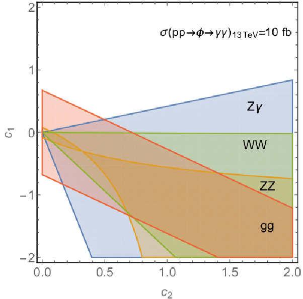
Refer to caption — Figure 1: Constraints on the coefficients of the dimension-5 operators, $c_{2}$ and $c_{1}$ . The shaded regions are excluded by the searches in the $8~{\rm TeV}$ data.

In this appendix, we analyze consistency between the diphoton signal at $13~{\rm TeV}$ and diboson searches at $8~{\rm TeV}$ , assuming general dimension-5 operators coupling a singlet scalar $\phi$ with the standard model gauge fields:

{\cal L}=\frac{\phi}{4\pi\Lambda}\biggl(g_{3}^{2}G^{a\mu\nu}\tilde{G}^{a}_{\mu\nu}+c_{2}g_{2}^{2}W^{b\mu\nu}\tilde{W}^{b}_{\mu\nu}+\frac{3c_{1}}{5}g_{1}^{2}B^{\mu\nu}\tilde{B}_{\mu\nu}\biggr).

(48)

(Our analysis applies if we replace $\tilde{G}^{a}_{\mu\nu}$ with $G^{a}_{\mu\nu}$ , and similarly for $\tilde{W}^{b}_{\mu\nu}$ and $\tilde{B}_{\mu\nu}$ .) We assume that the scalar $\phi$ is produced via gluon fusion and decays into standard model gauge bosons.

The constraint on each decay mode at the $8~{\rm TeV}$ LHC is given by³³ 3 To obtain the constraint from the $gg$ channel, we assume that the acceptance of the signal is $0.6$ , which is the case for an octet scalar decaying to two gluons.

\begin{array}[]{ll}\sigma_{pp\rightarrow\phi}B_{\phi\rightarrow\gamma\gamma}<2~{\rm fb}&\mbox{\cite[cite]{[\@@bibref{Number}{Aad:2015mna}{}{}]}}\\ \sigma_{pp\rightarrow\phi}B_{\phi\rightarrow Z\gamma}<5~{\rm fb}&\mbox{\cite[cite]{[\@@bibref{Number}{Aad:2014fha}{}{}]}}\\ \sigma_{pp\rightarrow\phi}B_{\phi\rightarrow ZZ}<30~{\rm fb}&\mbox{\cite[cite]{[\@@bibref{Number}{ATLAS_comb}{}{}]}}\\ \sigma_{pp\rightarrow\phi}B_{\phi\rightarrow W^{+}W^{-}}<80~{\rm fb}&\mbox{\cite[cite]{[\@@bibref{Number}{ATLAS_comb}{}{}]}}\\ \sigma_{pp\rightarrow\phi}B_{\phi\rightarrow gg}<5000~{\rm fb}&\mbox{\cite[cite]{[\@@bibref{Number}{Aad:2014aqa}{}{}]}}\end{array}

(49)

In Fig 1, we show the constraints on $c_{2}$ and $c_{1}$ from the $8~{\rm TeV}$ data, choosing $\Lambda$ such that the diphoton signal of $10~{\rm fb}$ is obtained at $13~{\rm TeV}$ . We find that the limits from the $Z\gamma$ and $ZZ$ modes are constraining. However, there is still a parameter region in which the observed diphoton excess at $13~{\rm TeV}$ is consistent with the limits from the $8~{\rm TeV}$ searches.

References

[1] M. Kado, “ATLAS results” Talk at ATLAS and CMS physics results from Run 2, CERN, Switzerland, December 15 (2015); ATLAS Collaboration, “Search for new physics decaying to two photons,” ATLAS-CONF-2015-081.
[2] J. Olsen, “CMS results,” Talk at ATLAS and CMS physics results from Run 2, CERN, Switzerland, December 15 (2015); CMS Collaboration, “Search for new physics in high mass diphoton events in proton-proton collisions at $13~{\rm TeV}$ ,” CMS-PAS-EXO-15-004.
[3] L. D. Landau, “On the angular momentum of a system of two photons,” Dokl. Akad. Nauk Ser. Fiz. 60, 207 (1948); C. N. Yang, “Selection rules for the dematerialization of a particle into two photons,” Phys. Rev. 77, 242 (1950).
[4] V. Agrawal, S. M. Barr, J. F. Donoghue and D. Seckel, “The anthropic principle and the mass scale of the standard model,” Phys. Rev. D 57, 5480 (1998) [hep-ph/9707380].
[5] G. Aad et al. [ATLAS Collaboration], “Search for pair production of a new heavy quark that decays into a $W$ boson and a light quark in $pp$ collisions at $\sqrt{s}=8~{\rm TeV}$ with the ATLAS detector,” arXiv:1509.04261 [hep-ex].
[6] A. Manohar and H. Georgi, “Chiral quarks and the nonrelativistic quark model,” Nucl. Phys. B 234, 189 (1984).
[7] R. D. Ball et al. [NNPDF Collaboration], “Parton distributions for the LHC Run II,” JHEP 04, 040 (2015) [arXiv:1410.8849 [hep-ph]].
[8] G. Aad et al. [ATLAS Collaboration], “Search for high-mass diphoton resonances in $pp$ collisions at $\sqrt{s}=8~{\rm TeV}$ with the ATLAS detector,” Phys. Rev. D 92, 032004 (2015) [arXiv:1504.05511 [hep-ex]]; CMS Collaboration, “Search for high-mass diphoton resonances in $pp$ collisions at $\sqrt{s}=8~{\rm TeV}$ with the CMS detector,” CMS-PAS-EXO-12-045.
[9] G. Aad et al. [ATLAS Collaboration], “Search for new resonances in $W\gamma$ and $Z\gamma$ final states in $pp$ collisions at $\sqrt{s}=8$ TeV with the ATLAS detector,” Phys. Lett. B 738, 428 (2014) [arXiv:1407.8150 [hep-ex]].
[10] C. Vafa and E. Witten, “Restrictions on symmetry breaking in vector-like gauge theories,” Nucl. Phys. B 234, 173 (1984).
[11] See, e.g., S. Weinberg, The Quantum Theory of Fields Volume II, (Cambridge University Press, Cambridge, United Kingdom, 1996).
[12] G. Aad et al. [ATLAS Collaboration], “Searches for heavy long-lived charged particles with the ATLAS detector in proton-proton collisions at $\sqrt{s}=8~{\rm TeV}$ ,” JHEP 01, 068 (2015) [arXiv:1411.6795 [hep-ex]]; S. Chatrchyan et al. [CMS Collaboration], “Searches for long-lived charged particles in pp collisions at $\sqrt{s}=7$ and $8~{\rm TeV}$ ,” JHEP 07, 122 (2013) [arXiv:1305.0491 [hep-ex]].
[13] H. Georgi and S. L. Glashow, “Unity of all elementary particle forces,” Phys. Rev. Lett. 32, 438 (1974).
[14] J. A. Aguilar-Saavedra, R. Benbrik, S. Heinemeyer and M. Pérez-Victoria, “Handbook of vectorlike quarks: mixing and single production,” Phys. Rev. D 88, 094010 (2013) [arXiv:1306.0572 [hep-ph]].
[15] L. J. Hall and Y. Nomura, “A finely-predicted Higgs boson mass from a finely-tuned weak scale,” JHEP 03, 076 (2010) [arXiv:0910.2235 [hep-ph]].
[16] C. Kilic, T. Okui and R. Sundrum, “Vectorlike confinement at the LHC,” JHEP 02, 018 (2010) [arXiv:0906.0577 [hep-ph]]; C. Kilic and T. Okui, “The LHC phenomenology of vectorlike confinement,” JHEP 04, 128 (2010) [arXiv:1001.4526 [hep-ph]].
[17] ATLAS collaboration, “Search for $WW$ , $WZ$ , and $ZZ$ resonances in $pp$ collisions at $\sqrt{s}=8~{\rm TeV}$ with the ATLAS detector,” ATLAS-CONF-2015-045.
[18] G. Aad et al. [ATLAS Collaboration], “Search for new phenomena in the dijet mass distribution using $p$ - $p$ collision data at $\sqrt{s}=8~{\rm TeV}$ with the ATLAS detector,” Phys. Rev. D 91, 052007 (2015) [arXiv:1407.1376 [hep-ex]].