Finding HeavyPaths in Weighted Graphs and a Case-Study on Community Detection

Graphs are convenient data structures for modeling real life data such as social networks, citation networks, the web, phone call and email histories, purchase/transaction records and user actions [1]. It is easy to model data with graphs. However, we need sophisticated tools to make sense of such data. In order to do so, we need to study notions such as connectivity [1], centrality [6] and density [28]. Graph algorithms are at the core of community detection, for discovering various types of groups based on previous interactions of individuals [39]. Random walk based methods have been used in many mining and graph applications. Mining interesting multi-relational patterns is solved as discovering maximal pseudo cliques in k-partite graphs [41].

A problem that has received relatively less attention in the research community is that of finding $k$ cycle-free heaviest paths of length $\ell$ in a weighted graph (HPP). Sum and product are examples of monotone aggregation functions that define the aggregate weight of a path. Generating lists of items of interest is a great practical example. Suppose edge probability $w_{(u,v)}=P(v|u)$, the conditional transition probability that a random user would like to listen to $u$ (as next song) given that $v$ is the current song. Also assume there is equal probability for any user to like any song. Using product as aggregation function, the weight of a path is directly proportional to the probability that a cycle free "chain" of songs appears one after another in a listening session. A heavy path in such graph, represents a playlist with high overall transition probability between songs. The graph can be created according to user(s) listening history. We can imagine other kinds of lists such as reading lists of books or papers that show flows of ideas through publications.

In influence networks, recently there have been attempts for sparcification [42]. A path with high probability is a highway for spreading influence in an influence network with transition probabilities on edges. A more principled approach takes into account only heavy paths rather than technicalities and complex problem definitions. A complete study of all of HPP applications goes beyond the scope of this paper. We need the preliminary work done in this paper, in order to aim at creating a toolbox that uses heavy paths for network analysis. Here, we show a possible novel application for community detection in research communities in a co-authorship network. We use maximal frequent sub-paths in top-$k$ heavy paths in order to discover the cores and further "grow" each core with peripheral nodes using existing edges in top paths. We enhance our observations with meta-data, and show that the core communities found using our approach unanimously report highly influential researchers.

We make the following contributions in the subsequent sections:

• •

  We formalize and motivate the HPP problem and show it is NP-hard and inapproximable. We discuss four exact algorithms, and provide a comparison of classical vs. novel algorithms for solving HPP. We provide a comprehensive experimental study of HPP algorithms presented in Section 7.

• •

  We present a case study to discover small but influential networks of people in research communities. We do this analysis on a sub-graph of DBLP co-authorship graph, and report the results in Section 6.

• •

  We show how a well studied top-$k$ query processing problem in the database literature can be converted to HPP on graphs where there is no database. We solely focus on algorithmic aspects, and propose a more scalable algorithm that overcomes the shortcommings of the Rankjoin [25] algorithm.

The most similar well studied problem to HPP in the literature is finding top-$k$ heavy paths on directed $\ell$-partite graphs. A nice example is $k\ell$-Stable Clusters problem [7]. Absence of cycles makes the studied problem considerably simpler than HPP. Furthermore, practical applications of HPP are not limited to $\ell$-partite graphs as described in Section 1. We show HPP is NP-hard and propose a practical algorithmic framework for solving it in the general case. It is common to use exponential time but efficient algorithms for mining purposes. Great examples are Apriori and FP-Growth [43], that is used for frequent item-set mining. Heavy paths also represent lists of highly connected items that can be used in similar ways to frequent item-sets and also for ordering of the items in the set.

Given a weighted graph $G(V,E,W)$, where weight $w_{(u,v)}$ represents the edge weight between $u$ and $v$, we aim at finding the $k$ heaviest simple paths of length $\ell$, with highest overall path weights. We call this the Heavy Path Problem (HPP).

A simple path of length $\ell$ is a sequence of nodes $(v_{0},\ldots,v_{\ell})$ such that $(v_{i},v_{i+1})\in E$, $0\leq i<\mbox{$\ell$}$, and there are no cycles, i.e., the nodes $v_{i}$ are distinct. Unless otherwise specified, in the rest of the paper, we use the term path to mean simple path. We focus on sum and product, as aggregation functions that define the weight of a path. For simplicity of presentation and practical considerations, we present using sum. We define weight of $P=(v_{0},...,v_{\ell})$, as $P.weight=\sum_{j=0}^{\ell-1}w_{(j,j+1)}$. Furthermore, we know we can convert product to sum using log values and this does not change the order of the list of top-$k$ heaviest paths.

Finding the heaviest path for a given parameter $\ell$ is equivalent to the $\ell$-TSP problem, defined as follows: Given a weighted graph, find a path of minimum weight that passes through any $\mbox{$\ell$}+1$ nodes. It is easy to see that for a given length $\ell$, a path $P$ is a solution to $\ell$-TSP iff it is a solution to HPP (with $k=1$) on the same graph but with edge weights modified as follows: let $w_{(u,v)}$ be the weight of an edge $(u,v)$ in the $\ell$-TSP instance; then the edge weight in the HPP instance is $w^{\prime}_{(u,v)}=C-w_{(u,v)}$, where $C$ is any constant. This reduction works in both ways given that we use the same constant $C$. We are not concerned with negative edge weights since we deal with paths without cycles; but, we focus on cases where edges are either all negative or all positive for simplicity. It is well known that $\ell$-TSP is NP-hard (as a version of TSP). Furthermore, $\ell$-TSP does not have any bounded approximation in the general case i.e. no triangle inequality on edge weights etc [2, 3].

In Figure 1, the heaviest simple path of length $4$, is obtained by visiting the nodes in the order 6–1–2–3–4 and has a weight of 3.35. In contrast, a different permutation of the nodes 4–3–6–1–2 has a weight of 3.08. The higher weight of a path can represent a sequence with more strength or better quality. Different permutations result in paths with different weights simply because paths consist of different edges most likely with different edge weights.

Limitation 1, simply follows the fact that paths are created using only sorted access to the list of edges. If we run SAA on the graph of Fig. 2, we won’t create the heaviest path (a,b,c,d) until the edge (c,d) is scanned. However, (c,d) is the lightest edge in the graph. This means following only sorted access, may delay the construction of the heaviest path until many irrelevant paths are created and discarded. This observation motivates the following optimization for finding heaviest paths.

In the example of Fig. 2, suppose we have constructed (a,b,c) and know it is the heaviest path of length $2$. It may be a good heuristic to extend (a,b,c) with new edges such as (c,d) and create paths of length $3$. Since (a,b,c) is the heaviest path of length $2$, it is very likely to create heavy paths of length $3$ by extending (a,b,c). Making access to graph edges such as (c,d), regardless of where they appear on the sorted list of edges, is what we refer to as "random access". An example of random access is presented by Figure 1(b). Making random access to the edge list simply means reading an edge without caring about where the edge is located on the sorted list of edges (through the adjacency matrix). This can help produce heavy paths containing low weight edges earlier. Our case study in Section 6, shows one practical example where a low weight edge on a heavy path, can have a meaningful interpretation. The discussion is provided in Section 6, for Gui-Rong Xue’s edges with others. Following this optimization, suppose we use random accesses to find “matching” edges with which to extend heaviest paths of length $\mbox{$\ell$}-1$ to length $\ell$. This way we won’t delay the creation of heavy paths until their lightest edge is visited under sorted access. However, this may not be enough for early termination of the algorithm. Another decisive factor in early termination is the upperbound threshold ($\theta$) value on weight of paths we have not created yet using the ScannedEdges.

SAA stops when $\theta$ gets smaller than the weight of the heaviest path of length $\ell$ discovered so far. Suppose there is an instance in which the heaviest path of length $\ell$ is lighter than $w_{min}+(\mbox{$\ell$}-1)\times w_{max}$. In this case, SAA will produce every path of length $\ell$ before reporting the heaviest path, resulting in no pruning. In Fig. 1, this happens when trying to find the heaviest path of length $4$ and in Fig. 2, when trying to find the heaviest path of length $3$. The following lemma highlights a natural possibility during the execution of SAA for obtaining a tighter threshold that results in earlier termination.

One way of making the threshold tighter is by keeping track of shorter paths. For example, if we know $P$ is a heaviest path of length $\mbox{$\ell$}-1$, we can infer that the heaviest path of length $\ell$ cannot be heavier than $P.weight+\mbox{$w_{max}$}$, a bound often much tighter than $w_{d}+(\mbox{$\ell$}-1)\mbox{$w_{max}$}$.

For this, we need to keep track of the heaviest paths of length $\mbox{$\ell$}-1$ one by one to lower the threshold more aggressively, gradually and smoothly. Pursuing this idea recursively leads to a framework where we maintain and release heaviest paths of each length $i$, $2\leq i\leq\mbox{$\ell$}$, at the right time and make the next threshold tighter. More precisely, we can perform the following optimization. For this purpose, we can use Buffers as sorted sets (priority queue) in order to store (insert) and release heavy paths (remove top).

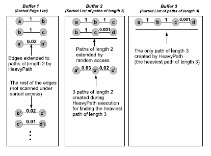
Figure 3 schematically describes the idea of using buffers for different path lengths. Buffer $B_{1}$ is the sorted edge list for the graph in Figure 2. Buffers $B_{2}$ and $B_{3}$ store paths of length 2 and 3 respectively. When random accesses are performed to extend paths of length $l-1$ to those of length $l$, the buffers can be used to store these intermediate paths. For instance, when the heaviest path of length 1 is seen, say edge $(a,b)$ is seen, it can be extended to paths of length 2 by accessing edges connected to its end points, as represented by $B_{2}$ in Figure 3. Similarly, the heaviest path of length 2 can be extended by an edge using random access to obtain path(s) in buffer $B_{3}$. Obviously, we do not extend all shorter path segments and extend only the one that is known to be the next heaviest path of shorter length in its own buffer. We describe this framework in more detail when we present the final algorithm next.

We start this section by providing an outline of our main algorithm for solving HPP. Our algorithm maintains a buffer $B_{i}$ for storing paths of length $i$ explored and not released ($P.w<\theta$), where $2\leq i\leq\mbox{$\ell$}$. Let threshold $\theta_{i}$ denote an upper bound on the weight of any path of length $i$ that has never been inserted into $B_{i}$. Algorithm 2 describes the overall approach. It takes as input a list of edges $E$ sorted in non-increasing order of edge weights, and parameters $\ell$ and $k$. It calls the NextHeavyPath method (Algorithm 3) repeatedly until the top-$k$ heaviest paths of length $\ell$ are found.

Algorithm 3¹¹ 1 In order to avoid StackOverflow we do a non-recursive implementation. We use the recursive pseudo code because it is more intuitive. describes the NextHeavyPath method. It takes as input a list of edges $E$ sorted in non-increasing order of edge weights, and the desired path length $l$, $l\geq 2$. It is a recursive algorithm that produces heaviest paths of shorter lengths on demand, and extends them with edges to produce paths of length $\ell$. The base case for this recursion is when $l=1$ and the algorithm reads the next edge from the sorted list of edges. The ReadEdge method returns the heaviest unseen edge in $E$ (sorted access, line 2). If $l<\mbox{$\ell$}$, the path of length $l$ obtained as a result of the recursion is extended by one hop to produce paths of length $l+1$. Specifically, a path of length $l<\mbox{$\ell$}$ is extended using edges (random access, lines 8 and 10) that can be appended to either one of its ends (returned by method EndNodes). The “+” operator for appending an edge to a path is defined in a way that guarantees no cycles are created. The threshold $\theta_{l}$ is updated aggressively when the next heaviest path of length $l-1$ is released from $B_{l-1}$. This is done by calling the method RemoveTopPath for buffer $B_{l-1}$ and returning the resulting path. If there is no path already in the buffer that beats $\theta_{l-1}$, this results in more recursion using smaller $l$, until this condition becomes true at some point during the execution. At any point during the execution if $i<\mbox{$\ell$}$ and the next heaviest path of length $i$ (P) has been obtained ($B_{i}.topScore>\theta_{i}$), $\theta_{i+1}$ is more intuitively updated as $\theta_{i+1}=P.W+W_{max}$ ²² 2 We use a bound tighter threshold, line $14$ of Algorithm $3$..

Suppose we have a co-authorship graph that connects researchers according to their publications. The edge weight is defined as the sum of "pairwise collaboration credits" that researchers get from each paper they publish together. Pairwise collaboration credit for a pair of authors in a paper, is $1/authorNum$. Where $authorNum$ is the number of authors of a paper. Given a collection of publications, we define an edge between two researchers if they have published at least one paper together. Then use the sum of "pairwise collaboration credits" they get from all of the papers they have published together as the edge weight. Single author papers do not contribute to edge weights. We further normalize edge weights by the maximum so that they are all in $[0,1]$. Using this graph, and given parameters $\ell$ and $k$ and a popularity ³³ 3 Same as support in frequent pattern mining parameter, we do the following,

1. 1.

   Find top-$k$ heaviest paths of length $l$

2. 2.

   Finding cores of communities: Find all maximal frequent sub-paths in top-$k$ paths. Frequent sub-paths are those that appear in more number of paths than the popularity parameter.

3. 3.

   Aggregate top-$k$ paths and form the aggregate graph of top paths

4. 4.

   Given a core and the aggregate graph of top paths, do the following: add any edges that connect any other researchers in the aggregate graph of top paths to the core. This shapes a community of core researchers that appear on many heavy paths. It also adds those other researchers who are strongly connected to the core community.

5. 5.

   Communities can grow using larger values for $k$ that adds more nodes to the picture. In a way, $k$ can be used to zoom in and zoom out of communities.

Using DBLP data [27], we constructed this graph using papers published between $2008$ and $2011$ (inclusive), presented in the main program one of these conferences: "SDM", "PKDD", "ICDM", "SIGKDD", "CIKM", "SIGIR", "ICML", "NIPS", "WWW" and "WSDM". Figure 4, shows two of the communities we find using parameters $l=5$, $k=100$ and $popularity=10$. We provide this graph (DBLPG), and the top-$100$ paths of length $5$, to enable the reader to reproduce the communities described ⁴⁴ 4 http://ucalgary.ca/$\scriptstyle\sim$mkhabbaz/DBLPG.zip. We notice that the core of community 1 (Figure 4(a)) contains the pair of researchers with the highest edge weight in the graph. This shows a long lasting collaboration. We did a quick google search about each of the core communities in DBLPG. Irwin King and Michael R. Lyu work for the Chinese University of Hong Kong. They are connected to Gui-Rong Xue who is the senior director at Aliyun.com and he is connected to a principal researcher from Microsoft research Asia (Zheng Chen).

Most of the researchers in community 2 (Figure 4(a)) have worked for Yahoo! Research Labs, including the three researchers in the core. Andrei Z. Broder is currently a distinguished scientist at Google. He has previously worked at Yahoo!, IBM and Altavista. We also found on his Wikipedia page that he is the inventor of MinHash locality sensitive hashing. Evgeniy Gabrilovich, is a senior staff research scientist at Google who also used to have a central role at Yahoo! research. Vanja Josifovski apparently still works for Yahoo! and is a Principal Research Scientist and the Lead of the Performance Advertising Group at Yahoo! Research. Most of the other researchers in community 2 work for yahoo! as their emails appear on their publications. Some may have moved to Google recently!

It is worth noting that we discovered three other cores as well in our output. Due to space limitations, we only report the cores: core 3 = $\{$Andrei Z. Broder, Evgeniy Gabrilovich, Xuerui Wang $\}$(weight = 0.73), core 4 = $\{$Shuicheng Yan, Ning Liu, Jun Yan, Zheng Chen $\}$ and core 5 = $\{$Ning Liu, Jun Yan, Zheng Chen, Weizhu Chen $\}$. Xuerui Wang is also a scientist at Yahoo! labs. Cores $4$ and $5$ have size $4$. We notice that a sub-path of length $3$ is shared between these two, with all researchers from Microsoft Research Asia. Community $1$ is connected to two of these three researchers through Gui-Rong Xue. This shows a potential for collaboration between these two cores in the future! who are the Chinese University of Hong Kong and Microsoft Research Asia. Changing the parameters $l$, $k$ and popularity, changes the output in the form presented in Figure 4(b). It can also help with creating a visualization tool that adapts its output with the current parameter values and be used for visualizing hierarchies and relationships of communities at different scales. Such a tool needs to run RSA repeatedly with different parameter values in order to change its view. This highlights the importance of scalability and efficiency for HPP problem. We leave the continuation and implementation of this idea to our future work.

The case study presented in this section, is also an example of an application where finding the exact solution is required. This is because we focus on $100$ heaviest paths and frequent pattern mining in order to discover the cores of communities. Heuristic or any sort of approximate solutions may result in paths that do not necessarily go through the cores that form the top communities. Top-$k$ heaviest paths, rely on their cores to be heavy!

Our theoretical results prove that HPP is np-hard and inapproximable in the general case. While it makes sense to seek more tractable problem definitions by adding constraints, still we show experimentally that we can achieve scalability practical enough for our main algorithm to be used in a real time fashion and be used in smart software technologies. We use a branch and bound solution for finding the exact solution, inspired by top-k algorithms. We use a constraint $\ell$, on edge weights and this makes our comparison for finding heavy paths, representing significantly important sequences in the graph more fair. Comparing path weights of paths with different lengths may not make enough sense in the general case. We show exact solution even for small $\ell$, if obtained, can be used in practice effectively, while other algorithms fail to report even for small $\ell$ in a timely manner. It is obviously nice to scale to longer paths and this requires smarter strategies for reducing $\theta$ during the execution that leads to faster search space pruning. We make a proposal for designing a network visualization tool-box with zoom-in and zoom-out functionalities with changing $k$. We find our presented case study practical but obviously as mentioned in Section 1, applications are not restricted to this and there are other applications such as those in bioinformatics. We can use high probability sequences in order to fix technology related errors such as replacing inaccurate or suspicious entries or filling in missing values in biological sequences. We can also use these high probability sequences for feature extraction from DNA which is an extremely long sequence of symbols in bioinformatics for classification and other learning tasks. One reason we choose visualizing bibliographic networks is presenting interpretable results for computer science audience. While there is a variety of solutions to be used in these applications, we want to propose a solution to a well-defined problem in computer science similar to TSP, that can be significantly leveraged for creating technologies in software industry. Another way to add constraints to the problem and make pruning more possible is through designing reliable heuristic algorithms with constraints on the distribution of edge weights. Of course, this requires careful testing for estimating distributions and we can focus on this extension in the future.

Recently, there have been advancements in the field of social networks described as Egonetworks ¹³¹³ 13 http://snap.stanford.edu/data/index.html. Egonetworks are typically presented as groups of people involved in different "circles". Our bibliographic network described in Section 6, is similar to the notion of circles in Egonetwork where each list of authors represents a circle. In an extreme scenario there may be many nodes involved in each circle in domains such as concrete social networks. Any problem definition for discovering dense or significant subgraphs according to such networks can result in finding significant sub-structures. We propose an effective approach for constructing such a graph. Based on the data available we prefer to make no judgement about the significance of individuals. Our proposed solution based on finding top-k heavy paths is proven to be scalable by experiments. On the other hands we can manage to change the output using simple parameters such as $k$, that enables us to zoom-in and zoom-out. Our argument for reliability of our output is the following observation. We notice many heavy paths share the same exact shorter sub-paths. This emphasizes the importance of some collaborations in the bibliographic network around which an important and successful research community is formed. This led to our definition of community detection approach that makes use of maximal frequent subpaths for discovering such frequent short paths shared among many top-k heavy paths. We follow the same approach for constructing graphs from Facebook and Twitter Egonetworks. In particular, we only use circles and convert mutual presence of nodes in circles to define edges. We find the same exact method described in Section 6, in order to define edge weights. Figure 9, reports the heaviest path weights of $\ell=1$ to $\ell=5$, and compares them with those obtained from DBLP data. We use the union of all circles first and then construct the graph. Since edge weights are all scaled to $(0-1)$, we expect heaviest paths of different length to be in the same range for all datasets. In comparison, we notice in Figure 9, that all graphs follow a similar curve for increasing $\ell$. We notice that the slope decreases with $\ell$, and it is quite likely path weight converges quickly for large $\ell$. This increases the chances of finding reliable heuristic algorithms with output close enough to the exact answer of the np-hard problem. Facebook and Twitter datasets result in paths with slightly heavier weights and we believe this is because in real life networks people with strong connections belong to many active networks while researchers may not be as socially active as ordinary people. Although the difference in path weights is small and almost negligible. The most notable facts to highlight are the similar shape of curves as well as the decreasing slope.

In [10], Hansen and Golbeck make a case for recommending playlists and other collections of items. The AutoDJ system of Platt et al. [11] is one of the early works on playlist generation that uses acoustic features of songs rather than a graph based representation. Random walk methods were used in [8], in order to generate lists of videos in a co-view graph. We formalized and presented our view of generating lists using random walks in introduction for recommending lists as an ordered package of items to users.

The HPP in a special case was studied recently by [7] and they defined a notion of Stable Clusters for the specific application of finding persistent chatter in the blogosphere. Unlike our setting, the graph associated with their application is $\ell$-partite and acyclic. Absence of cycles makes their technical problem more tractable than ours. The most efficient algorithm presented in their work is a BFS based method that follows a dynamic programming approach. We followed dynamic programming algorithm that also avoids cycles and found this approach extremely inefficient compared to RSA.

Rankjoin was first proposed by Ilyas et al. [26, 25, 24, 30, 33] to produce top-$k$ join tuples in a relational database. We show how to convert Rankjoin to HPP. Furthermore, no one has studied Rankjoin with self-joins to the best of our knowledge. In [4], authors provide a comprehensive summary of this algorithm and do optimality analysis as done in the theoretical database literature. Their conclusion is that beyond $\ell=2$, we can not guarantee any optimality results for Rankjoin. This also matches our results regarding HPP being np-hard and inapproximable.

Finding the top-$k$ heaviest paths in a graph is an interesting problem with many practical applications. We discuss the hardness of this problem. We focus on developing practical exact algorithms for this problem. We use an innovative top-$k$ query processing algorithm. We motivate the problem from several different perspectives and discuss possible applications. We present a case study on core community detection. Our findings suggest that our case study can be further extended to a community detection tool that discovers the key influential people in a network represented by a weighted graph. Our future work will focus on more applications of RSA, specially those in network analysis, community detection, recommender systems and bioinformatics. We would also like to investigate more scalable algorithms and threshold update strategies within the same framework. We also intend to design probabilistic and robust heuristic algorithms that work under memory and other types of constraints such as edge distribution.

References

- [1] Andrei Broader, Ravi Kumar, Farzin Maghoul, Prabhakar Raghavan, Sridhar Rajagopalan, Raymie Stata, Andrew Tomkins, Janet Wiener Graph Structure in the Web, Computer Networks, 2000.
- [2] N. Garg. et al. S. Arora and G. Karakostas. A 2 + epsilon approximation algorithm for the k-MST problem., Math. Prog., 2006.
- [3] N. Garg. et al. a 2-approximation for the k-mst problem in graphs., STOC, 2005.
- [4] Schnaitter, Karl and Polyzotis, Neoklis. Optimal algorithms for evaluating rank joins in database systems, TODS, 2010.
- [5] Schnaitter, Karl and Polyzotis, Neoklis. Evaluating rank joins with optimal cost, PODS, 2008.
- [6] U Kang, Spiros Papadimitriou, Jimeng Sun, Hanghang Tong. Centralities in Large Networks: Algorithms and Observations, SDM, 2011.
- [7] Bansal, Nilesh and Chiang, Fei and Koudas, Nick and Tompa, Frank Wm. Seeking stable clusters in the blogosphere, VLDB, 2007.
- [8] Shumeet Baluja, Rohan Seth, D. Sivakumar, Yushi Jing, Jay Yagnik, Shankar Kumar, Deepak Ravichandran, Mohamed Aly, Video suggestion and discovery for youtube: taking random walks through the view graph, WWW, 2008.
- [9] Fields, Ben and Rhodes, Christophe and d’Inverno, Mark, Using Song Social Tags and Topic Models to Describe and Compare Playlists, Workshop on Music Recommendation and Discovery, 2010.
- [10] Derek L. Hansen and Jennifer Golbeck, Mixing it up: recommending collections of items, CHI, 2009.
- [11] John C. Platt, Christopher J. C. Burges, S. Swenson, C. Weare, A. Zheng. Learning a Gaussian Process Prior for Automatically Generating Music Playlists, NIPS, 2001.
- [12] Hauver, D.B. and French, J.C. Web Delivering of Music, Flycasting: using collaborative filtering to generate a playlist for online radio, 2001.
- [13] Conor Hayes and Padraig Cunningham and Patrick Clerkin and Marco Grimaldi, Programme Driven Music Radio, ECAI, 2002.
- [14] Luke Barrington and Reid Oda and Gert Lanckriet, SMARTER THAN GENIUS? HUMAN EVALUATION OF MUSIC RECOMMENDER SYSTEMS, International Society for Music Information Retrieval, 2009.
- [15] Toni Cebrián and Marc Planagumà and Paulo Villegas and Xavier Amatriain, Music recommendations with temporal context awareness, RecSys, 2010.
- [16] Michael D. Ekstrand and Praveen Kannan and James A. Stemper and John T. Butler and Joseph A. Konstan and John Riedl, Automatically building research reading lists, RecSys, 2010.
- [17] Cai-Nicolas Ziegler and Sean M. McNee and Joseph A. Konstan and Georg Lausen, Improving recommendation lists through topic diversification, WWW, 2005.
- [18] X. Zhang and J. Chomicki, Preference Queries over Sets, IEEE International Conference on Data Engineering (ICDE), 2011.
- [19] Holger Bast and Debapriyo Majumdar and Ralf Schenkel and Martin Theobald and Gerhard Weikum, IO-Top-k: Index-access Optimized Top-k Query Processing, VLDB, 2006.
- [20] Measures of the Amount of Ecologic Association Between Species, Lee R. Dice, Ecology, 1945.
- [21] Hu, Yifan and Koren, Yehuda and Volinsky, Chris, Collaborative Filtering for Implicit Feedback Datasets, ICDM, 2008.
- [22] Yehuda Koen, Tutorial on recent progress in collaborative filtering, RecSys, 2008.
- [23] desJardins, M. and Eaton, E. and Wagstaff, K. L., Learning user preferences for sets of objects, ICML 2006.
- [24] Li, Chengkai and Chang, Kevin Chen-Chuan and Ilyas, Ihab F. and Song, Sumin, RankSQL: Query Algebra and Optimization for Relational Top-k Queries, SIGMOD, 2005.
- [25] Ilyas, Ihab F. and Shah, Rahul and Aref, Walid G. and Vitter, Jeffrey Scott and Elmagarmid, Ahmed K., Rank-aware query optimization, SIGMOD, 2004.
- [26] Ihab F. Ilyas and Walid G. Aref and Ahmed K. Elmagarmid, Supporting Top-k Join Queries in Relational Databases, VLDB, 2003.
- [27] Jie Tang, Jing Zhang, Limin Yao, Juanzi Li, Li Zhang, and Zhong Su. ArnetMiner, Extraction and Mining of Academic Social Networks., SIGKDD, 2008.
- [28] Gibson, David and Kumar, Ravi and Tomkins, Andrew, Discovering large dense subgraphs in massive graphs, VLDB, 2005.
- [29] M. Theobald, Gerhard Weikum, Ralf Schenkel, Top-k Query Evaluation with Probabilistic Guarantees., VLDB, 2004.
- [30] Jonathan Finger, Neoklis Polyzotis, Robust and Efficient Algorithms for Rank Join Evaluation, SIGMOD, 2009.
- [31] Johnson, David and Krishnan, Shankar and Chhugani, Jatin and Kumar, Subodh and Venkatasubramanian, Suresh, Compressing large boolean matrices using reordering techniques, VLDB, 2004.
- [32] Lappas, Theodoros and Liu, Kun and Terzi, Evimaria, Finding a team of experts in social networks, KDD, 2009.
- [33] Davide Martinenghi and Marco Tagliasacchi, Cost-Aware Rank Join with Random and Sorted Access, TKDE, 2011.
- [34] Ronald Fagin and Amnon Lotem and Moni Naor, Optimal Aggregation Algorithms for Middleware, J. of Comp. Sys. Sc., 2003.
- [35] Sanjeev Arora and George Karakostas, A 2 + approximation algorithm for the k-MST problem, Math. Prog., 2006.
- [36] A Dynamic Programming Approach to Sequencing Problems, Michael Held and Richard M. Karp, 1962.
- [37] Naveen Garg, Saving an epsilon: a 2-approximation for the k-MST problem in graphs, STOC, 2005.
- [38] M. Choudhury, M. Feldman, S. Amer-Yahia, N. Golbandi, R. Lempel, and C. Yu., Automatic construction of travel itineraries using social breadcrumbs., HT, 2010.
- [39] Community Detection in Graphs, Santo Fortunato, Physics Reports, 2009.
- [40] Mohsen Jamali, Martin Ester TrustWalker: a random walk model for combining trust-based and item-based recommendation., KDD, 2009.
- [41] Eirini Spyropoulou, Tijl De Bie, Interesting Multi-Relational Patterns., ICDM, 2011.
- [42] Michael Mathioudakis, Francesco Bonchi, Carlos Castillo, Aristides Gionis, Antti Ukkonen, Sparsification of Influence Networks., KDD, 2011.
- [43] Jiawei Han, Jian Pei, Yiwen Yin, Mining frequent patterns without candidate generation., SIGMOD, 2000.
- [44] Gerhard Weikum, Database Researchers: Plumbers or Thinkers?, EDBT, 2011.
- [45] Mohammad Khabbaz, Smriti Bhagat, Laks V. S. Lakshmanan, Finding Heavy Paths in Graphs: A Rank Join Approach., CoRR abs/1112.1117, 2011.
- [46] Hansen, Derek L. and Golbeck, Jennifer, Mixing it up: recommending collections of items, CHI 2009.
- [47] Mohammad Khabbaz and Smriti Bhagat and Laks V. S. Lakshmanan, Finding Heavy Paths in Graphs: A Rank Join Approach, Dept. of CS, UBC.
- [48] Chandra Chekuri and Martin P´al, A recursive greedy algorithm for walks in directed graphs, FOCS, 2005.