跳到论文正文
W Papers独立论文阅读器 arXiv:1512.03500 论文正文 计算阅读时间 · 0%
引用这篇论文根据当前论文元数据生成,正式投稿前建议核对。


License: arXiv.org perpetual non-exclusive license
arXiv:1512.03500v2 [stat.ME] 09 Aug 2018

Multi-threshold Accelerated Failure Time ModelT1

Jialiang Lim2label=e2]stalj@nus.edu.sg Email: [    Baisuo Jinm1label=e1]jbs@ustc.edu.cn Email: [ Affiliation: National University of Singapore\thanksmarkm2 and University of Science and Technology of China\thanksmarkm1 Address:  Department of Statistics and Applied Probability
National University of Singapore
Singapore,119077
E-mail:
Address:  Department of Statistics and Finance
University of Science and Technology of China
Hefei, Anhui, China, 230026
E-mail:
Abstract

A two-stage procedure for simultaneously detecting multiple thresholds and achieving model selection in the segmented accelerated failure time (AFT) model is developed in this paper. In the first stage, we formulate the threshold problem as a group model selection problem so that a concave 2-norm group selection method can be applied. In the second stage, the thresholds are finalized via a refining method. We establish the strong consistency of the threshold estimates and regression coefficient estimates under some mild technical conditions. The proposed procedure performs satisfactorily in our simulation studies. Its real world applicability is demonstrated via analyzing a follicular lymphoma data.

Keywords: 
threshold regression,
keywords
[class=MSC]
keywords
††email: e2††email: e1
\arxiv

arXiv:0000.0000

T1Supported by National Medical Research Council NMRC/CBRG/0014/2012 in Singapore, Academic Research Funding R-155-000-174-114 and National Natural Science Foundation of China (General Program, No. 11571337; Key Program, No. 71631006).

and

1 Introduction

Applied economists routinely test their models for the presence of structural change. If the evidence supports it, a threshold model is constructed and one needs to detect the thresholds (also called break points) at which to split the sample. The threshold variable may be an element of regressors. One such example is the well-known threshold autoregressive model (see Tong, 2012). Sometimes the threshold variable is simply the index of observed samples (eg. time in a time series model) and the model is commonly referred to as the change point model or segmented regression model (see Yao and Au, 1989, Perron, 2006, Fearnhead and Vasileiou, 2009).

In this paper we focus on the setting of multiple thresholds which is a much more challenging problem than a single break-point detection (Hansen, 2000). A number of issues arise in the presence of multiple change points. These include the determination of the number of breaks, estimation of the thresholds given the number, and statistical analysis of the resulting estimators. There exists a rich literature on this subject. For example, Inclan and Tiao (1994) identified multiple change-points of variance using the iterated cumulative sum of squares (ICSS) algorithm. Bai and Perron (2003) developed the dynamic programming principle for the estimation of multiple change-points in linear regression. Following the familiar idea of penalized estimation, Harchaoui and Lévy-Leduc (2010) used the least absolute shrinkage and selection operator (LASSO) algorithm to estimate the locations of multiple change-points, in one-dimensional piecewise constant signals. Davis et al. (2006) proposed a genetic algorithm to detect multiple break points, while recently Jin, Shi and Wu (2013) considered non-concave penalty functions including the smoothly clipped absolute deviation (SCAD) penalty and minimax concave penalty (MCP) penalty in piecewise stationary autoregressive processes. However, computational procedure and theoretical justification in Jin, Shi and Wu (2013) cannot be easily extended to survival analysis. We will consider a more difficult setting with censored event time in this paper. The theoretical results established in this paper are also more general than those in Jin, Shi and Wu (2013).

In life-testing research studies, single change point problem has been addressed by many authors. Specifically, Luo, Turnbull and Clark (1997) considered the Cox model with a change point at an unknown time and established asymptotic results for maximum partial likelihood estimates. Pons (2003) studied unknown threshold of a predictor variable under Cox model using counting processes theory while Kosorok and Song (2007) further examined the more sophisticated linear transformation models and provided necessary inference tools. Very few authors considered the problem of estimating multiple thresholds for survival regression analysis. Censored lifetime data break down the usual estimation framework for completely observed data. We usually cannot attain a closed-form solution for regression estimates and therefore face an increased complexity of estimating thresholds accurately. To address this under-developed issue, we consider the accelerated failure time (AFT) model as a typical example of regression models in this paper and contribute a new methodology on change-point problem for survival data analysis.

The AFT model permits a direct assessment of the covariate effects on the survival time, facilitating the interpretation of regression coefficients for the mean response. There are many estimation methods available for AFT model in the literature, including Buckley and James (1979), Prentice (1978), Tsiatis (1990), Ying (1993), Lin, Wei and Ying (1998). Many estimation methods for right censored data are rank-based and in practice the estimating functions may be discontinuous, producing challenges to the computation. In contrast, Stute (1993, 1996) proposed a weighted least squares estimator for AFT model, and established the consistency and asymptotic normality under technical conditions. Huang, Ma and Xie (2006) carried out a variable selection procedure and estimation in AFT model with high-dimensional covariates based on Stute’s estimator. Xia, Jiang, Li and Zhang (2016) also employed Stute’s estimator for nonparametric variable screening and selection. In this paper, we formally adopt the Stute estimator to study the parameter estimation for the AFT model with ss thresholds, where s≥0s\geq 0 is unspecified. Using a two-stage procedure proposed in this paper we may estimate the thresholds and the regression coefficients simultaneously. Interestingly our procedure may be straight forwardly extended to incorporate variable selection for high-dimensional data analysis.

The paper is arranged as follows. In Section 2, the multiple break-point problem for the AFT model is formulated. We then propose a two-stage procedure to detect the thresholds and estimate model parameters. In Section 3, we establish theoretical properties of our procedure. Next simulation studies are conducted in Section 4 to examine the performance of our methods. An empirical application to a follicular lymphomais data is presented in Section 5.

Throughout the paper, 𝟏q=(1,…,1)⊤{\mathbf{1}}_{q}=(1,\ldots,1)^{\top} is a qq-dimensional constant vector, IqI_{q} is the q×qq\times q identity matrix, 1{⋅}1_{\{\cdot\}} is an indicator function, 𝑨⊤{\mbox{\boldmath$A$}}^{\top} is the transpose of a matrix 𝑨A, and ⌊c⌋\lfloor c\rfloor is the integer part of a real number cc. For a vector 𝐚\mathbf{a}, 𝐚⊤\mathbf{a}^{\top} is its transpose, aja_{j} is its jjth component, |𝐚||\mathbf{a}| and ‖𝐚‖\|\mathbf{a}\| are respectively its L1L_{1}-norm and L2L_{2}-norm. If 𝒜\mathcal{A} is a set, its complement and its size are denoted by 𝒜c{\mathcal{A}}^{c} and ♯​𝒜\sharp\mathcal{A}, respectively. In addition, “→a.s.\rightarrow_{a.s.}” denotes convergence with probability 1.

2 Methodology for multiple thresholds under AFT model

Let Ti,i=1,…,nT_{i},i=1,\ldots,n be the independent logarithm of the failure time and 𝐗1,…,𝐗n\mathbf{X}_{1},\ldots,\mathbf{X}_{n} are i.i.d. pp-dimensional regressors. Assume (Ti,𝐗i),i=1,…,n(T_{i},\mathbf{X}_{i}),i=1,\ldots,n, satisfy the following AFT model with ss thresholds located at a1<…<asa_{1}<\ldots<a_{s}:

Ti\displaystyle T_{i} =\displaystyle= ∑j=1s+1𝐗i⊤βj∗1{aj−1<Zi≤aj}+εi\displaystyle\sum_{j=1}^{s+1}\mathbf{X}_{i}^{\top}\mathbf{\beta}_{j}^{*}1_{\{a_{j-1}<Z_{i}\leq a_{j}\}}+\varepsilon_{i} (2.1)
=\displaystyle= 𝐗i⊤[β1∗+∑ℓ=1s𝐝ℓ∗1{aℓ<Zi⩽as+1}]+εi,i=1,…,n\displaystyle\mathbf{X}_{i}^{\top}\left[\mathbf{\beta}_{1}^{*}+\sum_{\ell=1}^{s}\mathbf{d}_{\ell}^{*}1_{\{a_{\ell}<Z_{i}\leqslant a_{s+1}\}}\right]+\varepsilon_{i},\hskip 9.24994pti=1,\ldots,n
=\displaystyle= {𝐗i⊤​β1∗+εiif ​a0<Zi≤a1,𝐗i⊤​(β1∗+𝐝1∗)+εiif ​a1<Zi≤a2,……𝐗i⊤​(β1∗+∑ℓ=1s𝐝ℓ∗)+εi,if ​as<Zi≤as+1,\displaystyle{\begin{cases}\mathbf{X}_{i}^{\top}\mathbf{\beta}_{1}^{*}+\varepsilon_{i}&\mbox{if }a_{0}<Z_{i}\leq a_{1},\\ \mathbf{X}_{i}^{\top}(\mathbf{\beta}_{1}^{*}+\mathbf{d}_{1}^{*})+\varepsilon_{i}&\mbox{if }a_{1}<Z_{i}\leq a_{2},\\ \ldots&\ldots\\ \mathbf{X}_{i}^{\top}\left(\mathbf{\beta}_{1}^{*}+\sum_{\ell=1}^{s}\mathbf{d}_{\ell}^{*}\right)+\varepsilon_{i},&\mbox{if }a_{s}<Z_{i}\leq a_{s+1},\end{cases}}

where β1∗,…,βs+1∗\mathbf{\beta}_{1}^{*},\ldots,\mathbf{\beta}_{s+1}^{*} are unknown pp-dimensional regression coefficients for s+1s+1 subgroups, 𝐝ℓ∗=βℓ+1∗−βℓ∗,ℓ=1,…,s\mathbf{d}_{\ell}^{*}=\mathbf{\beta}_{\ell+1}^{*}-\mathbf{\beta}_{\ell}^{*},\ell=1,\ldots,s, are the increments of coefficients between two adjacent subgroups, s≥0s\geq 0 is the unknown number of thresholds, ZiZ_{i} is the thresholding variable, a1,…,asa_{1},\ldots,a_{s} are unknown threshold locations, a0=0a_{0}=0, as+1=na_{s+1}=n, ε1,…,εn\varepsilon_{1},\ldots,\varepsilon_{n} are independent random errors, and εaℓ−1+1,…,εaℓ\varepsilon_{a_{\ell-1}+1},\ldots,\varepsilon_{a_{\ell}} , the subgroup in the series {εi,i=1,…,n}\{\varepsilon_{i},i=1,\ldots,n\} separated by the threshold locations {aℓ,ℓ=1,…,s}\{a_{\ell},\ell=1,\ldots,s\}, are identically distributed with mean zero and variance σℓ2\sigma_{\ell}^{2}, ℓ=1,…,s+1\ell=1,\ldots,s+1. Notice that if s=0s=0, the model (2.1) does not involve threshold. If s≥1s\geq 1, we denote P(Zi≤aj)=τj,j=1,…,sP(Z_{i}\leq a_{j})=\tau_{j},j=1,\ldots,s where 0<τ1<τ2<…<τs<10<\tau_{1}<\tau_{2}<\ldots<\tau_{s}<1. If Zi=iZ_{i}=i, we retain the usual change point model, and the condition P⁡(Zi≤aj)=τjP(Z_{i}\leq a_{j})=\tau_{j} will be replaced by aj/n→τja_{j}/n\to\tau_{j} since change point locations actually depend on the sample size in this setting. Figure 1 is an example of model (2.1), where s=2s=2, ZZ is generated from a normal distribution and TT is generated from a mixture normal distribution.
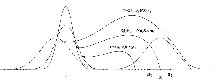
Refer to caption
Figure 1: An example of model (2.1)

Let Ci,i=1,…,nC_{i},i=1,\ldots,n be logarithm of the censoring time which are assumed to be independent and identically distributed (i.i.d.). In practice we only observe (Yi,δi,𝐗i),i=1,…,n(Y_{i},\delta_{i},\mathbf{X}_{i}),i=1,\ldots,n, where Yi=min⁡(Ti,Ci)Y_{i}=\min(T_{i},C_{i}) is the censored logarithm of the failure time and δi=1{Ti≤Ci}\delta_{i}=1_{\{T_{i}\leq C_{i}\}} is the censoring indicator.

Throughout this paper, let Y(1,ℐ)≤…≤Y(b,ℐ)Y_{(1,\mathcal{I})}\leq\ldots\leq Y_{(b,\mathcal{I})} be the ordered failure times in the index set ℐ\mathcal{I} and b=♯​ℐb=\sharp\mathcal{I}. Let δ[ℓ,ℐ]\delta_{[\ell,\mathcal{I}]} be the concomitant of the ℓ\ellth-ordered Y(ℓ,ℐ),ℓ=1,…,bY_{(\ell,\mathcal{I})},\ell=1,\ldots,b. Define the Kaplan-Meier weights as

w[1,ℐ]=δ[1,ℐ]b,w[ℓ,ℐ]=δ[ℓ,ℐ]b−ℓ+1∏k=1ℓ−1(b−kb−k+1)δ[k,ℐ],ℓ=2,…,b.w_{[1,\mathcal{I}]}=\frac{\delta_{[1,\mathcal{I}]}}{b},w_{[\ell,\mathcal{I}]}=\frac{\delta_{[\ell,\mathcal{I}]}}{b-\ell+1}\prod_{k=1}^{\ell-1}\big(\frac{b-k}{b-k+1}\big)^{\delta_{[k,\mathcal{I}]}},\qquad\ell=2,\ldots,b.

Such weights are constructive elements of the Kaplan-Meier estimator for the survival function (See Lawless, 2011). Let rYi,ℐ∈[1,b]r_{Y_{i},\mathcal{I}}\in[1,b] be the rank of YiY_{i} among {Yi:i∈ℐ}\{Y_{i}:i\in\mathcal{I}\} i.e. Yi=Y(rYi,ℐ,ℐ)Y_{i}=Y_{(r_{Y_{i},\mathcal{I}},\mathcal{I})}, i∈ℐi\in\mathcal{I}. For simplicity, we denote Y(rYi,ℐ)=Y(rYi,ℐ,ℐ)=YiY_{(r_{Y_{i},\mathcal{I}})}=Y_{(r_{Y_{i},\mathcal{I}},\mathcal{I})}=Y_{i} and w[rYi,ℐ]=w[rYi,ℐ,ℐ]w_{[r_{Y_{i},\mathcal{I}}]}=w_{[r_{Y_{i},\mathcal{I}},\mathcal{I}]}.

If aj,j=1,…,sa_{j},j=1,\ldots,s are known, define ℐj∗={i:aj−1<Zi≤aj}\mathcal{I}_{j}^{*}=\{i:a_{j-1}<Z_{i}\leq a_{j}\} and bj∗=♯​ℐj∗b_{j}^{*}=\sharp\mathcal{I}_{j}^{*}, we can use the Stute estimator to fit the AFT model. The resulting estimator β^1∗,𝐝^1∗,…,𝐝^s∗\mathbf{\hat{\beta}}_{1}^{*},\mathbf{\hat{d}}_{1}^{*},\ldots,\mathbf{\hat{d}}_{s}^{*} may be represented by a weighted least squares estimator that minimizes

∑j=1s+1bj∗2​n​∑i∈ℐj∗w[rYi,ℐj∗]​(Yi−𝐗i⊤​(β1∗+∑k=1j−1𝐝k∗))2.\displaystyle\sum_{j=1}^{s+1}\frac{b_{j}^{*}}{2n}\sum_{i\in\mathcal{I}_{j}^{*}}w_{[r_{Y_{i},\mathcal{I}_{j}^{*}}]}\left(Y_{i}-\mathbf{X}_{i}^{\top}(\mathbf{\beta}_{1}^{*}+\sum_{k=1}^{j-1}\mathbf{d}_{k}^{*})\right)^{2}. (2.2)

We note that the weights {w[rYi,ℐj∗]}\{w_{[r_{Y_{i},\mathcal{I}_{j}^{*}}]}\} depend on the order of the random failure times and hence the related asymptotic argument is not as standard as the independent and identically distributed (i.i.d.) case in linear regression.

We intend to estimate ss, a1a_{1}, …\ldots, and asa_{s} and then use the detected change point(s) to obtain the Stute estimator for regression coefficients. To this end, first we need to decide the total number of thresholds and the approximate distances between pairs of thresholds. After that we may proceed to determine the exact locations of thresholds. We propose a two-stage procedure in the following sections.

2.1 The Splitting Stage

First we split the data sequence into qn+1q_{n}+1 segments where qnq_{n} tends to infinity as n→∞n\to\infty. Let {Zi:δi=1,i=1,…,n}={Z~1,…,Z~n∗}\{Z_{i}:\delta_{i}=1,i=1,\ldots,n\}=\{\tilde{Z}_{1},\ldots,\tilde{Z}_{n^{*}}\} where n∗=∑i=1nδin^{*}=\sum_{i=1}^{n}\delta_{i} is the total number of events. In order to allow each segment to include enough failure event observations, the data sequence is split such that the first segment ℐ1={i:Zi≤Z~(n∗−qn​m)}\mathcal{I}_{1}=\{i:Z_{i}\leq\tilde{Z}_{(n^{*}-q_{n}m)}\} involves n∗−qn​mn^{*}-q_{n}m events, and each of the other qnq_{n} segments ℐj={i:Z~(n∗−(qn−j+2)​m)<Zi≤Z~(n∗−(qn−j+1)​m)},j=2,…,qn+1\mathcal{I}_{j}=\{i:\tilde{Z}_{(n^{*}-(q_{n}-j+2)m)}<Z_{i}\leq\tilde{Z}_{(n^{*}-(q_{n}-j+1)m)}\},j=2,\ldots,q_{n}+1 involve mm events where m=⌈n∗/qn⌉m=\lceil n^{*}/q_{n}\rceil and Z~(1)≤Z~(2)​…≤Z~(n∗)\tilde{Z}_{(1)}\leq\tilde{Z}_{(2)}\ldots\leq\tilde{Z}_{(n^{*})} are the ordered threshold variables associated with subjects no failed. Define bj=♯ℐj,j=1,…,qn+1b_{j}=\sharp\mathcal{I}_{j},j=1,\ldots,q_{n}+1.

To select these intervals covering thresholds {aj}\{a_{j}\}, we propose a concave 2-norm group selection method, such that an estimate θ^=(β^1⊤,𝐝^1⊤,…,𝐝^qn⊤)⊤\hat{\mathbf{\theta}}=(\hat{\mathbf{\beta}}_{1}^{\top},\hat{\mathbf{d}}_{1}^{\top},\ldots,\hat{\mathbf{d}}_{q_{n}}^{\top})^{\top} is given by minimizing

∑j=1qn+1bj2​n​∑i∈ℐjw[rYi,ℐj]​(Yi−𝐗i⊤​(β1+∑k=1j−1𝐝k))2+∑k=1qnpλn,γn​(‖𝐝k‖),\displaystyle\sum_{j=1}^{q_{n}+1}\frac{b_{j}}{2n}\sum_{i\in\mathcal{I}_{j}}w_{[r_{Y_{i},\mathcal{I}_{j}}]}\left(Y_{i}-\mathbf{X}_{i}^{\top}(\mathbf{\beta}_{1}+\sum_{k=1}^{j-1}\mathbf{d}_{k})\right)^{2}+\sum_{k=1}^{q_{n}}p_{\lambda_{n},\gamma_{n}}(\|\mathbf{d}_{k}\|), (2.3)

where λn>0\lambda_{n}>0, γn>1\gamma_{n}>1 are tuning parameters, and the penalty function pλn,γn​(|u|)>0p_{\lambda_{n},\gamma_{n}}(|u|)>0 is concave in |u||u|. For the simplicity of presentation, we shall only consider two well-studied penalty functions in this paper, namely the smoothly clipped absolute deviation (SCAD) penalty and the minimax concave penalty (MCP). SCAD was introduced in Fan and Li (2001) and defined as pλ,γ​(u)=λ​u​I[0,λ]​(u)+γ​λ​u−0.5​(u2+λ2)γ−1​I(λ,γ​λ]​(u)+λ2​(γ2−1)2​(γ−1)​I(γ​λ,∞)​(u),γ>1.p_{\lambda,\gamma}(u)=\lambda uI_{[0,\;\lambda]}(u)+\frac{\gamma\lambda u-0.5(u^{2}+\lambda^{2})}{\gamma-1}I_{(\lambda,\;\gamma\lambda]}(u)+\frac{\lambda^{2}(\gamma^{2}-1)}{2(\gamma-1)}I_{(\gamma\lambda,\;\infty)}(u),\gamma>1. MCP was introduced in Zhang (2010) and defined as pλ,γ​(u)=(λ​u−u22​γ)​I[0,γ​λ]​(u)+12​γ​λ2​I(γ​λ,∞)​(u),γ>2.p_{\lambda,\gamma}(u)=(\lambda u-\displaystyle\frac{u^{2}}{2\gamma})I_{[0,\;\gamma\lambda]}(u)+\displaystyle\frac{1}{2}\gamma\lambda^{2}I_{(\gamma\lambda,\;\infty)}(u),\gamma>2.

Let 𝐘(j)=(Yi,i∈ℐj)⊤\mathbf{Y}_{(j)}=(Y_{i},i\in\mathcal{I}_{j})^{\top}, 𝐗(j)=(𝐗i,i∈ℐj)⊤\mathbf{X}_{(j)}=(\mathbf{X}_{i},i\in\mathcal{I}_{j})^{\top}, 𝐰~(j)=bj​(w[rYi,ℐj],i∈ℐj)⊤\tilde{\mathbf{w}}_{(j)}=b_{j}(w_{[r_{Y_{i},\mathcal{I}_{j}}]},i\in\mathcal{I}_{j})^{\top}, 𝐲~(j)=d​i​a​g​(𝐰~(j))1/2​𝐘(j)\tilde{\mathbf{y}}_{(j)}=diag(\tilde{\mathbf{w}}_{(j)})^{1/2}\mathbf{Y}_{(j)}, 𝐗~(j)=d​i​a​g​(𝐰~(j))1/2​𝐗(j)\tilde{\mathbf{X}}_{(j)}=diag(\tilde{\mathbf{w}}_{(j)})^{1/2}\mathbf{X}_{(j)}, j=1,…,qn+1j=1,\ldots,q_{n}+1. Denote 𝐲~=(𝐲~(1)⊤,…,𝐲~(qn+1)⊤)⊤\tilde{\mathbf{y}}=(\tilde{\mathbf{y}}_{(1)}^{\top},\ldots,\tilde{\mathbf{y}}_{(q_{n}+1)}^{\top})^{\top}, 𝐗~=(𝐗~(1),…,𝐗~(qn+1))\tilde{\mathbf{X}}=(\tilde{\mathbf{X}}^{(1)},\ldots,\tilde{\mathbf{X}}^{(q_{n}+1)}) where 𝐗~(1)=(𝐗~(1)⊤,…,𝐗~(qn+1)⊤)⊤\tilde{\mathbf{X}}^{(1)}=(\tilde{\mathbf{X}}_{(1)}^{\top},\ldots,\tilde{\mathbf{X}}_{(q_{n}+1)}^{\top})^{\top} and 𝐗~(j)=(𝟎p×∑i=1j−1bi,𝐗~(j)⊤CLOSE\tilde{\mathbf{X}}^{(j)}=({\bf 0}_{p\times\sum_{i=1}^{j-1}b_{i}},\tilde{\mathbf{X}}_{(j)}^{\top}, …\ldots, OPEN𝐗~(qn+1)⊤)⊤\tilde{\mathbf{X}}_{(q_{n}+1)}^{\top})^{\top}, j=2,…j=2,\ldots, qn+1q_{n}+1. The estimator θ^\hat{\mathbf{\theta}} in (2.3) can be written as

θ^=arg⁡minθ​{12​n​‖𝐲~−𝐗~​θ‖2+∑j=1qnpλn,γn​(‖𝐝j‖)},\displaystyle\hat{\mathbf{\theta}}=\arg\min_{\mathbf{\theta}}\left\{\frac{1}{2n}\|\tilde{\mathbf{y}}-\tilde{\mathbf{X}}\mathbf{\theta}\|^{2}+\sum_{j=1}^{q_{n}}p_{\lambda_{n},\gamma_{n}}(\|\mathbf{d}_{j}\|)\right\}, (2.4)

We apply the group coordinate descent (GCD) algorithm to estimate θ^n\hat{\theta}_{n} from (2.4).

The properties of θ^\hat{\theta} will be given by Theorem 3.2 in the next section. For simplicity, we write θ^=(θ^1⊤,…,θ^qn+1⊤)⊤\hat{\mathbf{\theta}}=(\hat{\mathbf{\theta}}_{1}^{\top},\ldots,\hat{\mathbf{\theta}}_{q_{n}+1}^{\top})^{\top} such that θ^1=β^1\hat{\mathbf{\theta}}_{1}=\hat{\mathbf{\beta}}_{1} and θ^j=𝐝^j−1\hat{\mathbf{\theta}}_{j}=\hat{\mathbf{d}}_{j-1}, j=2,…,qn+1j=2,\ldots,q_{n}+1. Let 𝒜^={j:θ^j≠0,j=1,…,qn+1}\hat{\mathcal{A}}=\{j:\hat{\mathbf{\theta}}_{j}\neq 0,j=1,\ldots,q_{n}+1\}, and 𝒜^∗\hat{\mathcal{A}}^{*} be a subset of 𝒜^\hat{\mathcal{A}} such that 𝒜^∗={j:j∈𝒜^,j−1∉𝒜^,j=2,…,qn+1}={k^1,…,k^s^}\hat{\mathcal{A}}^{*}=\{j:j\in\hat{\mathcal{A}},j-1\not\in\hat{\mathcal{A}},j=2,\ldots,q_{n}+1\}=\{\hat{k}_{1},\ldots,\hat{k}_{\hat{s}}\}. If s^=0\hat{s}=0, we declare there is no threshold. If s^>0\hat{s}>0, by Theorem 3.2, the true threshold aja_{j} is highly likely to be located in (Z~(n∗−(qn−k^j+3)​m),Z~(n∗−(qn−k^j+1)​m)](\tilde{Z}_{(n^{*}-(q_{n}-\hat{k}_{j}+3)m)},\tilde{Z}_{(n^{*}-(q_{n}-\hat{k}_{j}+1)m)}], j=1,…,s^j=1,\ldots,\hat{s}.

2.2 The Refining Stage

If s^>0\hat{s}>0, by Theorem 3.2, we can estimate the threshold aja_{j} in (Z~(n∗−(qn−k^j+3)​m)CLOSE(\tilde{Z}_{(n^{*}-(q_{n}-\hat{k}_{j}+3)m)}, Z~(n∗−(qn−k^j+1)​m)]\tilde{Z}_{(n^{*}-(q_{n}-\hat{k}_{j}+1)m)}]. To obtain the estimates of the thresholds {aj}\{a_{j}\}, we denote ℐ^j={i:Z~(n∗−(qn−k^j+3)​m)<Zi≤Z~(n∗−(qn−k^j+1)​m)}\hat{\mathcal{I}}_{j}=\{i:\tilde{Z}_{(n^{*}-(q_{n}-\hat{k}_{j}+3)m)}<Z_{i}\leq\tilde{Z}_{(n^{*}-(q_{n}-\hat{k}_{j}+1)m)}\}, ℐ^j,ς−={i:Z~(n∗−(qn−k^j+3)​m)<Zi≤ς}\hat{\mathcal{I}}_{j,\varsigma^{-}}=\{i:\tilde{Z}_{(n^{*}-(q_{n}-\hat{k}_{j}+3)m)}<Z_{i}\leq\varsigma\}, ℐ^j,ς+={i:ς<Zi≤Z~(n∗−(qn−k^j+1)​m)}\hat{\mathcal{I}}_{j,\varsigma^{+}}=\{i:\varsigma<Z_{i}\leq\tilde{Z}_{(n^{*}-(q_{n}-\hat{k}_{j}+1)m)}\}

Qj​(ς−,β)\displaystyle Q_{j}(\varsigma^{-},\mathbf{\beta}) =\displaystyle= ♯​ℐ^j,ς−♯​ℐ^j​∑i∈ℐ^j,ς−w[rYi,ℐ^j,ς−]​(Yi−𝐗i⊤​β)2,\displaystyle\frac{\sharp\hat{\mathcal{I}}_{j,\varsigma^{-}}}{\sharp\hat{\mathcal{I}}_{j}}\sum_{i\in\hat{\mathcal{I}}_{j,\varsigma^{-}}}w_{[r_{Y_{i},\hat{\mathcal{I}}_{j,\varsigma^{-}}}]}(Y_{i}-\mathbf{X}_{i}^{\top}\mathbf{\beta})^{2},
Qj​(ς+,β)\displaystyle Q_{j}(\varsigma^{+},\mathbf{\beta}) =\displaystyle= ♯​ℐ^j,ς+♯​ℐ^j​∑i∈ℐ^j,ς+w[rYi,ℐ^j,ς+]​(Yi−𝐗i⊤​β)2,\displaystyle\frac{\sharp\hat{\mathcal{I}}_{j,\varsigma^{+}}}{\sharp\hat{\mathcal{I}}_{j}}\sum_{i\in\hat{\mathcal{I}}_{j,\varsigma^{+}}}w_{[r_{Y_{i},\hat{\mathcal{I}}_{j,\varsigma^{+}}}]}(Y_{i}-\mathbf{X}_{i}^{\top}\mathbf{\beta})^{2},

and use the following method to estimate aja_{j}:

a^j=argminς∈(Z~(n∗−(qn−k^j+3)​m),Z~(n∗−(qn−k^j+1)​m)]​⋂{Z(1),…,Z(n)}​{Qj​(ς)},\displaystyle\hat{a}_{j}=\mbox{argmin}_{\varsigma\in(\tilde{Z}_{(n^{*}-(q_{n}-\hat{k}_{j}+3)m)},\tilde{Z}_{(n^{*}-(q_{n}-\hat{k}_{j}+1)m)}]\bigcap\{Z_{(1)},\ldots,Z_{(n)}\}}\{Q_{j}(\varsigma)\}, (2.5)

where Qj​(ς)=minβ⁡Qj​(ς−,β)+minβ⁡Qj​(ς+,β)Q_{j}(\varsigma)=\min_{\mathbf{\beta}}Q_{j}(\varsigma^{-},\mathbf{\beta})+\min_{\mathbf{\beta}}Q_{j}(\varsigma^{+},\mathbf{\beta}), j=1,…,s^j=1,\ldots,\hat{s}, and Z(1)≤Z(2)​…≤Z(n)Z_{(1)}\leq Z_{(2)}\ldots\leq Z_{(n)} are the order of Zi,i=1,…,nZ_{i},i=1,\ldots,n . The regions separated by the thresholds achieve the overall minimum least squares errors. The consistency of a^j\hat{a}_{j} will be provided in Theorem 3.3.

2.3 Remarks

After we obtain a^j,j=1,…,s^\hat{a}_{j},j=1,\ldots,\hat{s} by (2.5), it is sensible to use the weighted least squares to obtain a final estimate of the coefficients in model (2.1). Let ℐ^j∗={i:a^j−1<Zi≤a^j}\hat{\mathcal{I}}^{*}_{j}=\{i:\hat{a}_{j-1}<Z_{i}\leq\hat{a}_{j}\} and b^j∗=♯​ℐ^j∗\hat{b}_{j}^{*}=\sharp\hat{\mathcal{I}}^{*}_{j}, j=1,…,s^+1j=1,\ldots,\hat{s}+1 where a^0=−∞\hat{a}_{0}=-\infty and a^s^+1=+∞\hat{a}_{\hat{s}+1}=+\infty. Then the coefficient θ∗=((β1∗)⊤,(𝐝1∗)⊤,…,(𝐝s^∗)⊤)⊤=(θ1∗,…,θp⁡(s^+1)∗)⊤\mathbf{\theta}^{*}=((\mathbf{\beta}^{*}_{1})^{\top},(\mathbf{d}_{1}^{*})^{\top},\ldots,(\mathbf{d}_{\hat{s}}^{*})^{\top})^{\top}=(\theta_{1}^{*},\ldots,\theta_{p(\hat{s}+1)}^{*})^{\top} can be estimated by minimizing the following penalized least squares

M⁡(θ)=∑j=1s^n+1b^j∗2​n​∑i∈ℐ^j∗w[rYi,ℐ^j∗]​(Yi−𝐗i⊤​(β1+∑k=1j−1𝐝k))2+∑i=1p⁡(s^n+1)pλn,γn​(|θi|),\displaystyle M(\mathbf{\theta})=\sum_{j=1}^{\hat{s}_{n}+1}\frac{\hat{b}_{j}^{*}}{2n}\sum_{i\in\hat{\mathcal{I}}^{*}_{j}}w_{[r_{Y_{i},\hat{\mathcal{I}}^{*}_{j}}]}\left(Y_{i}-\mathbf{X}_{i}^{\top}(\mathbf{\beta}_{1}+\sum_{k=1}^{j-1}\mathbf{d}_{k})\right)^{2}+\sum_{i=1}^{p(\hat{s}_{n}+1)}p_{\lambda_{n},\gamma_{n}}(|\theta_{i}|), (2.6)

where the penalty function pλn,γn​(|u|)>0p_{\lambda_{n},\gamma_{n}}(|u|)>0 is the same as in (2.4) and θ=(β1⊤,𝐝1⊤,…,𝐝s^⊤)⊤=(θ1,…,θp⁡(s^+1))⊤\mathbf{\theta}=(\mathbf{\beta}_{1}^{\top},\mathbf{d}_{1}^{\top},\ldots,\mathbf{d}_{\hat{s}}^{\top})^{\top}=(\theta_{1},\ldots,\theta_{p(\hat{s}+1)})^{\top}. The inclusion of the penalty functions may lead to a sparse solution since the number of parameters could be quite large for all the subgroups. The oracle property of θ^∗=arg⁡minθ⁡M⁡(θ)\hat{\mathbf{\theta}}^{*}=\arg\min_{\mathbf{\theta}}M(\mathbf{\theta}) will be given by Theorem 3.3.

Similar to Jin, Shi and Wu (2013), γn\gamma_{n} is set as 2.4 for SCAD and MCP penalties . The regularization parameter λn\lambda_{n} can be chosen by the Bayesian information criterion (BIC).

The performance of θ^∗\hat{\mathbf{\theta}}^{*} is further dependent on the segment length mm. The selection of an optimal mm can be carried out as follows: Apply the splitting stage to the data sequence LL times with the common segment length of events (excluding the first segment) mℓm_{\ell}, ℓ=1,…,L\ell=1,\ldots,L. In order to meet the assumption, i.e., m=⌊c​n⌋m=\lfloor c\sqrt{n}\rfloor made in Theorem 3.2, we set mℓ=⌊κℓ​n⌋m_{\ell}=\lfloor\kappa_{\ell}\sqrt{n}\rfloor, ℓ=1,…,L\ell=1,\ldots,L, where κℓ\kappa_{\ell} takes values from LL grid-points in an interval, say [0.1, 2.0]. For each mℓm_{\ell}, applying the proposed two-stage procedure, we obtain the set of estimated thresholds ℳ^ℓ={a^1,ℓ,…,a^s^ℓ,ℓ}\hat{\mathcal{M}}_{\ell}=\{\hat{a}_{1,\ell},\ldots,\hat{a}_{\hat{s}_{\ell},\ell}\}, ℓ=1,…,L\ell=1,\ldots,L. We use the BIC to choose the best index

ℓ^=argminℓ=1,…,L​{B​I​Cℳ^ℓ},\hat{\ell}=\mbox{argmin}_{\ell=1,\ldots,L}\left\{BIC_{\hat{\mathcal{M}}_{\ell}}\right\}, (2.7)

where

B​I​Cℳ^ℓ=\displaystyle BIC_{\hat{\mathcal{M}}_{\ell}}= n​log⁡(∑j=1s^ℓ+1♯​ℐ^j,ℓn​(min⁡∑i∈ℐ^j,ℓβ⁡w[rYi,ℐ^j,ℓ]​(Yi−𝐗i⊤​β)2))\displaystyle n\log\left(\sum_{j=1}^{\hat{s}_{\ell}+1}\frac{\sharp\hat{\mathcal{I}}_{j,\ell}}{n}\left(\min_{\mathbf{\beta}}\sum_{i\in\hat{\mathcal{I}}_{j,\ell}}w_{[r_{Y_{i},\hat{\mathcal{I}}_{j,\ell}}]}(Y_{i}-\mathbf{X}_{i}^{\top}\mathbf{\beta})^{2}\right)\right)
+q⁡(s^ℓ+1)​log⁡(n)\displaystyle+q(\hat{s}_{\ell}+1)\log(n) (2.8)

with ℐ^j,ℓ={i:a^j−1,ℓ<Zi≤a^j,ℓ}\hat{\mathcal{I}}_{j,\ell}=\{i:\hat{a}_{j-1,\ell}<Z_{i}\leq\hat{a}_{j,\ell}\}, a^0,ℓ=−∞,a^s^ℓ+1,ℓ=+∞\hat{a}_{0,\ell}=-\infty,\hat{a}_{\hat{s}_{\ell}+1,\ell}=+\infty. The optimal mo​p​t=⌊κℓ^​n⌋{m}_{opt}=\lfloor\kappa_{\hat{\ell}}\sqrt{n}\rfloor and the optimal estimated thresholds ℳ^o​p​t={a^1,ℓ^,…,a^s^ℓ^,ℓ^}\hat{\mathcal{M}}_{opt}=\{\hat{a}_{1,\hat{\ell}},\ldots,\hat{a}_{\hat{s}_{\hat{\ell}},\hat{\ell}}\}.

We refer to the proposed two-stage procedure as Two Stage Multiple Change-points Detection (TSMCD) from now on. Since two regularization methods, i.e. MCP, and SCAD, will be utilized in the splitting stage, we refer to the corresponding TSMCD as TSMCD(MCP) and TSMCD(SCAD), respectively. The detailed algorithm of TSMCP is described in the following table.

Algorithm 1 TSMCD
1: for ℓ=1,2,…,20\ell=1,2,\ldots,20 do Step 1: Splitting stage
2:   Set m=⌊0.1​ℓ​n∗⌋m=\lfloor 0.1\ell\sqrt{n^{*}}\rfloor and qn=⌊n∗/m⌋−1q_{n}=\lfloor n^{*}/m\rfloor-1 where n∗n^{*} is the number of events;
3:   Split the data sequence into qn+1q_{n}+1 segments ℐj,j=1,…,qn+1\mathcal{I}_{j},j=1,\ldots,q_{n}+1 as Section 2.1;
4:   Estimate θ^=((θ^1)⊤,…,(θ^qn+1)⊤)⊤\hat{\mathbf{\theta}}=((\hat{\mathbf{\theta}}_{1})^{\top},\ldots,(\hat{\mathbf{\theta}}_{q_{n}+1})^{\top})^{\top} by minimizing (2.3) or (2.4);
5:   Compute the index sets 𝒜^={j:θ^j≠0,j=1,…,qn+1}\hat{\mathcal{A}}=\{j:\hat{\mathbf{\theta}}_{j}\neq 0,j=1,\ldots,q_{n}+1\} and 𝒜^∗={j:j∈𝒜^,j−1∉𝒜^,j=2,…,qn+1}≡{k^1,…,k^s^}\hat{\mathcal{A}}^{*}=\{j:j\in\hat{\mathcal{A}},j-1\not\in\hat{\mathcal{A}},j=2,\ldots,q_{n}+1\}\equiv\{\hat{k}_{1},\ldots,\hat{k}_{\hat{s}}\} where k^1<k^2<…<k^s^\hat{k}_{1}<\hat{k}_{2}<\ldots<\hat{k}_{\hat{s}} and s^=♯​𝒜^∗\hat{s}=\sharp\hat{\mathcal{A}}^{*}; Step 2: Refining stage
6:   if s^=0\hat{s}=0 then go to the step 9;
7:   else if s^>0\hat{s}>0 then estimate the threshold aja_{j} in (Z~(n∗−(qn−k^j+3)​m)CLOSE(\tilde{Z}_{(n^{*}-(q_{n}-\hat{k}_{j}+3)m)}, Z~(n∗−(qn−k^j+1)​m)]\tilde{Z}_{(n^{*}-(q_{n}-\hat{k}_{j}+1)m)}] by (2.5);
8:   end if
9:   Estimate the coefficient θ∗=((β1∗)⊤,(𝐝1∗)⊤,…,(𝐝s^∗)⊤)⊤\mathbf{\theta}^{*}=((\mathbf{\beta}^{*}_{1})^{\top},(\mathbf{d}_{1}^{*})^{\top},\ldots,(\mathbf{d}_{\hat{s}}^{*})^{\top})^{\top} by minimizing (2.6);
10:   Return the set of estimated thresholds ℳ^ℓ={a^1,ℓ,…,a^s^ℓ,ℓ}\hat{\mathcal{M}}_{\ell}=\{\hat{a}_{1,\ell},\ldots,\hat{a}_{\hat{s}_{\ell},\ell}\} in step 7 and the estimator of the coefficient θ^ℓ∗\hat{\mathbf{\theta}}^{*}_{\ell} in step 9, and compute B​I​Cℳ^ℓBIC_{\hat{\mathcal{M}}_{\ell}} by (2.8);
11: end for
12: Choose ℓ^\hat{\ell} that minimizes the B​I​Cℳ^ℓBIC_{\hat{\mathcal{M}}_{\ell}} and obtain the final estimators ℳ^o​p​t=ℳ^ℓ^\hat{\mathcal{M}}_{opt}=\hat{\mathcal{M}}_{\hat{\ell}} and θ^o​p​t∗=θ^ℓ^∗\hat{\mathbf{\theta}}^{*}_{opt}=\hat{\mathbf{\theta}}^{*}_{\hat{\ell}}.

3 Asymptotic theory

Under model (2.1), we further denote the distributions of {Ti,i∈ℐj∗}\{T_{i},i\in\mathcal{I}_{j}^{*}\} and {Yi,i∈ℐj∗}\{Y_{i},i\in\mathcal{I}_{j}^{*}\} to be FjF_{j} and HjH_{j}, j=1,…,s+1j=1,\ldots,s+1. Denote the distribution of log censoring times {c1,…,cn}\{c_{1},\ldots,c_{n}\} by GG. We define UFj,UHjU_{F_{j}},U_{H_{j}} and UGU_{G} to be the least upper bound for the support of Fj,HjF_{j},H_{j} and GG, respectively.

Throughout the paper the following assumption will be made:

  • (A1)

    P⁡(Zi≤aj)=τjP(Z_{i}\leq a_{j})=\tau_{j} where 0<τ1<τ2<…<τs<10<\tau_{1}<\tau_{2}<\ldots<\tau_{s}<1, E⁡(εi|𝐗i)=0E(\varepsilon_{i}|\mathbf{X}_{i})=0, E⁡(Ti2)<∞E(T_{i}^{2})<\infty, E⁡(𝐗i​𝐗i⊤)=Σ0E(\mathbf{X}_{i}\mathbf{X}_{i}^{\top})=\Sigma_{0} is finite and nonsingular, and ZiZ_{i} and εi\varepsilon_{i} are independent, i=1,…,ni=1,\ldots,n.

  • (A2)

    TiT_{i} and CiC_{i} are independent, HjH_{j} is continuous, and censoring mechanism is independent of covariates.

  • (A3)

    UFj<UGU_{F_{j}}<U_{G} or UFj=UG=∞U_{F_{j}}=U_{G}=\infty.

Assumption (A1) allows heteroscedastic error. For example, we may relax the error assumption to be εi=σ⁡(𝐗i⊤​βj∗)​εi∗\varepsilon_{i}=\sigma(\mathbf{X}_{i}^{\top}\mathbf{\beta}_{j}^{*})\varepsilon_{i}^{*} where εi∗\varepsilon_{i}^{*} is independent with 𝐗i\mathbf{X}_{i} and ε1∗,…,εn∗\varepsilon_{1}^{*},\ldots,\varepsilon_{n}^{*} are i.i.d. with mean zero and variance σ2\sigma^{2}. (A2) assumes that δi\delta_{i} is conditionally independent of 𝐗i\mathbf{X}_{i} given TiT_{i}. (A3) implies that UHj=UFjU_{H_{j}}=U_{F_{j}}.

We first present a result for the simple case where s=1s=1 is known. Tentatively we rewrite a1a_{1} and 𝐝1∗\mathbf{d}_{1}^{*} as aa and 𝐝∗\mathbf{d}^{*}, respectively, in model (2.1), and replace τ1\tau_{1} with τ\tau in assumption (A1) for simplicity.

Theorem 3.1.

Assume conditions (A1)-(A3) hold for model (2.1), s=1s=1 is known and ‖𝐝∗‖>0\|\mathbf{d}^{*}\|>0. Let a^=argminς∈{Z(1),…,Z(n)}{minβ♯​ℐ^ς−n∑i∈ℐ^ς−w[rYi,ℐ^ς−]\hat{a}=\mbox{argmin}_{\varsigma\in\{Z_{(1)},\ldots,Z_{(n)}\}}\{\min_{\mathbf{\beta}}\frac{\sharp\hat{\mathcal{I}}_{\varsigma^{-}}}{n}\sum_{i\in\hat{\mathcal{I}}_{\varsigma^{-}}}w_{[r_{Y_{i},\hat{\mathcal{I}}_{\varsigma^{-}}}]} (Yi−𝐗i⊤β)2+minβ♯​ℐ^ς+n∑i∈ℐ^ς+w[rYi,ℐ^ς+](Yi−𝐗i⊤β)2}(Y_{i}-\mathbf{X}_{i}^{\top}\mathbf{\beta})^{2}+\min_{\mathbf{\beta}}\frac{\sharp\hat{\mathcal{I}}_{\varsigma^{+}}}{n}\sum_{i\in\hat{\mathcal{I}}_{\varsigma^{+}}}w_{[r_{Y_{i},\hat{\mathcal{I}}_{\varsigma^{+}}}]}(Y_{i}-\mathbf{X}_{i}^{\top}\mathbf{\beta})^{2}\} where ℐ^ς−={i:Zi≤ς}\hat{\mathcal{I}}_{\varsigma^{-}}=\{i:Z_{i}\leq\varsigma\} and ℐ^ς+={i:ς<Zi}\hat{\mathcal{I}}_{\varsigma^{+}}=\{i:\varsigma<Z_{i}\}, then we have 1n∑i=1n1{Zi≤a^}→a.s.τ\frac{1}{n}\sum_{i=1}^{n}1_{\{Z_{i}\leq\hat{a}\}}\to_{a.s.}\tau as n→∞n\to\infty. Furthermore, if ZiZ_{i} is a continuous random variable, we have a^→a.s.a\hat{a}\to_{a.s.}a; if Zi=iZ_{i}=i, we have a^/n→a.s.τ\hat{a}/n\to_{a.s.}\tau.

The proof of Theorem 3.1 is given in the Appendix. The result itself may be of interest since many econometric studies deal with a single change point.

If s≥0s\geq 0 is unknown, we use the proposed TSMCD to estimate ss, and the change points aj,j=1,…,sa_{j},j=1,\ldots,s when s>0s>0. The following technical conditions are also needed:

  • (A4)

    m→∞m\to\infty and m=O⁡((n∗)r)m=O((n^{*})^{r}), where 0<r≤1/20<r\leq 1/2 is a constant.

  • (A5)

    The penalty function pλn,γn​(|u|)p_{\lambda_{n},\gamma_{n}}(|u|) of (2.4) satisfies pλn,γn​(0)=0p_{\lambda_{n},\gamma_{n}}(0)=0, pλn,γn′​(u)p_{\lambda_{n},\gamma_{n}}^{\prime}(u) =0=0 if u>γn​λnu>\gamma_{n}\lambda_{n}, pλn,γn′​(0)=λnp_{\lambda_{n},\gamma_{n}}^{\prime}(0)=\lambda_{n}, λn→0\lambda_{n}\rightarrow 0 and λn​n/log⁡n→∞\lambda_{n}\sqrt{n}/\log n\rightarrow\infty as n→∞n\to\infty.

  • (A6)

    εi=σ(𝐗i⊤βj∗)εi∗,i∈ℐj∗,j=1,…,s+1\varepsilon_{i}=\sigma(\mathbf{X}_{i}^{\top}\mathbf{\beta}_{j}^{*})\varepsilon_{i}^{*},i\in\mathcal{I}^{*}_{j},j=1,\ldots,s+1, εi∗\varepsilon_{i}^{*} is independent of 𝐗i\mathbf{X}_{i}, ε1∗,…,εn∗\varepsilon_{1}^{*},\ldots,\varepsilon_{n}^{*} are i.i.d. random errors with distribution F0F_{0}. Suppose UF0<UFjU_{F_{0}}<U_{F_{j}}, and there exists some positive constant UFj∗<UFj−UF0U_{F_{j}}^{*}<U_{F_{j}}-U_{F_{0}}, such that σ⁡(𝐗i⊤​βj∗)=0\sigma(\mathbf{X}_{i}^{\top}\mathbf{\beta}_{j}^{*})=0 if 𝐗⊤​βj∗>UFj∗\mathbf{X}^{\top}\mathbf{\beta}_{j}^{*}>U_{F_{j}}^{*}, otherwise σ⁡(𝐗i⊤​βj∗)=1\sigma(\mathbf{X}_{i}^{\top}\mathbf{\beta}_{j}^{*})=1, j=1,…,s+1j=1,\ldots,s+1.

By law of large numbers and Assumption (A1), P⁡(Zi≤aj)=τjP(Z_{i}\leq a_{j})=\tau_{j} implies

∑i=1n1{aj−1<Zi≤aj}/n→a.s.τj−τj−1>0.\sum_{i=1}^{n}1_{\{a_{j-1}<Z_{i}\leq{a}_{j}\}}/n\to_{a.s.}\tau_{j}-\tau_{j-1}>0.

Assumption (A4) implies with probability 1

∑i=1n1{Z~(n∗−(qn−j+2)​m)<Zi≤Z~(n∗−(qn−j+1)​m)}/n=m/n∗→0.\sum_{i=1}^{n}1_{\{\tilde{Z}_{(n^{*}-(q_{n}-j+2)m)}<Z_{i}\leq\tilde{Z}_{(n^{*}-(q_{n}-j+1)m)}\}}/n=m/n^{*}\to 0.

Thus Assumption (A1) and (A4) ensure that there is at most one threshold in each segment {Zi:Z~(n∗−(qn−j+2)​m)<Zi≤Z~(n∗−(qn−j+1)​m)}\{Z_{i}:\tilde{Z}_{(n^{*}-(q_{n}-j+2)m)}<Z_{i}\leq\tilde{Z}_{(n^{*}-(q_{n}-j+1)m)}\} for sufficiently large nn where Z~(n∗−(qn−j+2)​m)\tilde{Z}_{(n^{*}-(q_{n}-j+2)m)} and Z~(n∗−(qn−j+1)​m)\tilde{Z}_{(n^{*}-(q_{n}-j+1)m)}, j=1,…,qn+1j=1,\ldots,q_{n}+1, are defined in Section 2.1. Both SCAD and MCD satisfy the penalty assumption (A5). (A6) implies Ti=𝐗i⊤​βj∗T_{i}=\mathbf{X}_{i}^{\top}\mathbf{\beta}_{j}^{*} if UFj∗+UF0<Yi≤UFjU_{F_{j}}^{*}+U_{F_{0}}<Y_{i}\leq U_{F_{j}}.

Define 𝒜∗={i1,…,ia}{\mathcal{A}}^{*}=\{i_{1},\ldots,i_{a}\} to be the group index set and 𝐗~𝒜∗=(𝐗~(i1),…CLOSE,\tilde{\mathbf{X}}_{\mathcal{A}^{*}}=(\tilde{\mathbf{X}}^{(i_{1})},\ldots, OPEN𝐗~(ia))\tilde{\mathbf{X}}^{(i_{a})}) . Similarly we can define θ^𝒜∗\hat{\mathbf{\theta}}_{\mathcal{A}^{*}} and θ^(𝒜∗)c\hat{\mathbf{\theta}}_{(\mathcal{A}^{*})^{c}}. Let 𝒜={1,kj,n,kj,n+1:j=1,…,s}\mathcal{A}=\{1,k_{j,n},k_{j,n}+1:j=1,\ldots,s\}.

Theorem 3.2.

If Assumptions (A1)-(A6) hold, min{||β1∗||,||𝐝1∗||,…,\min\{||\mathbf{\beta}_{1}^{*}||,||\mathbf{d}_{1}^{*}||,\ldots, ||𝐝s∗||}||\mathbf{d}_{s}^{*}||\} >2​p​γ​λn>2\sqrt{p}\gamma\lambda_{n}, then with probability 1, (2.4) has a local minimizer θ^\hat{\mathbf{\theta}} such that θ^𝒜∗=(𝐗~𝒜∗⊤​𝐗~𝒜∗)−1​𝐗~𝒜∗⊤​𝐲~\hat{\mathbf{\theta}}_{\mathcal{A}^{*}}=(\tilde{\mathbf{X}}_{\mathcal{A}^{*}}^{\top}\tilde{\mathbf{X}}_{\mathcal{A}^{*}})^{-1}\tilde{\mathbf{X}}_{\mathcal{A}^{*}}^{\top}\tilde{\mathbf{y}} and θ^(𝒜∗)c=𝟎\hat{\mathbf{\theta}}_{(\mathcal{A}^{*})^{c}}=\mathbf{0}, where

𝒜∗⊆𝒜and1∈𝒜∗,kℓ,n∈𝒜∗orkℓ,n+1∈𝒜∗for allℓ=1,…,s.\displaystyle\mathcal{A}^{*}\subseteq\mathcal{A}~\textrm{and}~1\in\mathcal{A}^{*},k_{\ell,n}\in\mathcal{A}^{*}~\textrm{or}~k_{\ell,n}+1\in\mathcal{A}^{*}~\textrm{for all}~\ell=1,\ldots,s. (3.1)

The proof of Theorem 3.2 is given in Appendix. Theorem 3.2 provides the existence of the solution of (2.4). In this theorem, 𝒜∗\mathcal{A}^{*} is the group index set of no-zero group elements of θ^\hat{\mathbf{\theta}}. By (3.1), 𝒜∗\mathcal{A}^{*} is not unique and may take 2s2^{s} possible forms.

Let 𝐚=(a1,…,as)⊤\mathbf{a}=(a_{1},\ldots,a_{s})^{\top} be the vector of threshold locations and 𝐚^=(a^1,…,a^s^)⊤\mathbf{\hat{a}}=(\hat{a}_{1},\ldots,\hat{a}_{\hat{s}})^{\top} is obtained by (2.5). Similar to the definition of 𝐲~\tilde{\mathbf{y}} and 𝐗~\tilde{\mathbf{X}}, replacing ℐj\mathcal{I}_{j} with ℐj∗\mathcal{I}_{j}^{*} or ℐ^j∗\mathcal{\hat{I}}_{j}^{*} and then we may define 𝐲~𝐚\tilde{\mathbf{y}}_{\mathbf{a}} or 𝐲~𝐚^\tilde{\mathbf{y}}_{\mathbf{\hat{a}}} and 𝐗~𝐚\tilde{\mathbf{X}}_{\mathbf{a}} or 𝐗~𝐚^\tilde{\mathbf{X}}_{\mathbf{\hat{a}}} . By Assumption (A1), we have 1n𝐗~𝐚⊤𝐗~𝐚→a.sΓ\frac{1}{n}\tilde{\mathbf{X}}_{\mathbf{a}}^{\top}\tilde{\mathbf{X}}_{\mathbf{a}}\rightarrow_{a.s}\Gamma, where Γ\Gamma is a positive definite matrix.

To obtain the limiting property of θ^∗\hat{\mathbf{\theta}}^{*} in (2.6), we will further need the following assumption:

  • (A7)

    maxu≥0⁡{pλn,γn′′​(u)}+λ(s+1)​p​(Γ)>0\max_{u\geq 0}\{p_{\lambda_{n},\gamma_{n}}^{\prime\prime}(u)\}+\lambda_{(s+1)p}(\Gamma)>0 where λ(s+1)​p​(Γ)\lambda_{(s+1)p}(\Gamma) is the minimal eigenvalue of Γ\Gamma.

For MCP, (A7) is equivalent to λ(s+1)​p​(Γ)>1/γ\lambda_{(s+1)p}(\Gamma)>1/\gamma, and for SCAD, (A7) is equivalent to λ(s+1)​p​(Γ)>1/(γ−1)\lambda_{(s+1)p}(\Gamma)>1/(\gamma-1). Let (θ1∗,…,θ(s+1)​p∗)⊤=(\theta_{1}^{*},\ldots,\theta_{(s+1)p}^{*})^{\top}= ((β1∗)⊤,(𝐝1∗)⊤CLOSE((\mathbf{\beta}_{1}^{*})^{\top},(\mathbf{d}_{1}^{*})^{\top} ,OPEN…,(𝐝s∗)⊤)⊤\ldots,(\mathbf{d}_{s}^{*})^{\top})^{\top} and 𝒮={j:θj∗≠0,j=1,…,(s+1)p}\mathcal{S}=\{j:\theta^{*}_{j}\neq 0,j=1,\ldots,(s+1)p\}.

Let 𝒜^={j:θ^j≠0,j=1,…,qn+1}\hat{\mathcal{A}}=\{j:\hat{\mathbf{\theta}}_{j}\neq 0,j=1,\ldots,q_{n}+1\}, and 𝒜^∗\hat{\mathcal{A}}^{*} be a subset of 𝒜^\hat{\mathcal{A}} such that 𝒜^∗={j:j∈𝒜^,j−1∉𝒜^,j=2,…,qn+1}={k^1,…,k^s^}\hat{\mathcal{A}}^{*}=\{j:j\in\hat{\mathcal{A}},j-1\not\in\hat{\mathcal{A}},j=2,\ldots,q_{n}+1\}=\{\hat{k}_{1},\ldots,\hat{k}_{\hat{s}}\} where s^\hat{s} is the size of 𝒜^∗\hat{\mathcal{A}}^{*}.

Theorem 3.3.

Under the Assumptions (A1)-(A7), minj∈S⁡{|θj|}>γ​λn\min_{j\in S}\{|\theta_{j}|\}>\gamma\lambda_{n}, θ^\hat{\mathbf{\theta}} is the local minimizer in Theorem 3.2, ZiZ_{i} is a continuous random variable and θ^∗\hat{\mathbf{\theta}}^{*} is a minimizer of M⁡(θ)M(\theta) given by (2.6), then we have, with probability 1,

  • (1)

    s^=s\hat{s}=s;

  • (2)

    𝐚^→𝐚;\mathbf{\hat{a}}\to\mathbf{a};

  • (3)

    θ^∗=θ^o\hat{\mathbf{\theta}}^{*}=\hat{\mathbf{\theta}}^{o},

where θ^o=argminθ{∥𝐲~𝐚^−𝐗~𝐚^θ∥2:θ=(θ1,…,θ(s+1)​p)⊤,θj=0∀j∉𝒮}\hat{\mathbf{\theta}}^{o}=\arg\min_{\mathbf{\theta}}\{\|\tilde{\mathbf{y}}_{\mathbf{\hat{a}}}-\tilde{\mathbf{X}}_{\mathbf{\hat{a}}}\mathbf{\theta}\|^{2}:\mathbf{\theta}=(\theta_{1},\ldots,\theta_{(s+1)p})^{\top},\theta_{j}=0~\forall~j\not\in\mathcal{S}\} is the oracle estimator when thresholds and the set 𝒮\mathcal{S} are known.

The proof of Theorem 3.3 is also given in Appendix. We attain the consistency of the TSMCD estimators in this theorem. Our estimators work as well as the oracle estimators in large samples.

4 Simulation Study

We generate random samples from model (2.1) with s=2s=2 thresholds in the following. Specifically, we generate the regressors 𝐗i=(x1,i,x2,i,…,x6,i)⊤\mathbf{X}_{i}=(x_{1,i},x_{2,i},\ldots,x_{6,i})^{\top} with x1,i=1x_{1,i}=1, xj,i∼N(0,1),j=2,…,6x_{j,i}\sim N(0,1),j=2,\ldots,6, and εi∼N⁡(0,0.5)\varepsilon_{i}\sim N(0,0.5). We specify the coefficients (θ1∗,…,θ18∗)⊤=((β1∗)⊤,(𝐝1∗)⊤,(𝐝2∗)⊤)⊤=(2,1,1,1,1,1,−1,0,0,−1,−1,−1,0,−1,1,0,0,0)⊤(\theta_{1}^{*},\ldots,\theta_{18}^{*})^{\top}=((\mathbf{\beta}_{1}^{*})^{\top},(\mathbf{d}_{1}^{*})^{\top},(\mathbf{d}_{2}^{*})^{\top})^{\top}=(2,1,1,1,1,1,-1,0,0,-1,-1,-1,0,-1,1,0,0,0)^{\top}, the threshold variable Zi=x2,iZ_{i}=x_{2,i}, and true thresholds a1=−0.5244a_{1}=-0.5244, a2=0.2533a_{2}=0.2533. The two thresholds are the 30% and 60% lower percentiles of the standard normal distribution. We first design the following four cases:
Example 1: n=150n=150, xj,i,j=2,…,6x_{j,i},j=2,\ldots,6 are independent and censoring variable Ci∼N⁡(2,16)C_{i}\sim N(2,16);
Example 2: The same setting as Example 1 except n=300n=300;
Example 3: The same setting as Example 2 except Ci∼N⁡(∑j=26xj,i,16)C_{i}\sim N(\sum_{j=2}^{6}x_{j,i},16);
Example 4: The same setting as Example 3 except covariance between xj1,ix_{j_{1},i} and xj2,ix_{j_{2},i} is 0.5|j1−j2|0.5^{|j_{1}-j_{2}|}.

The censoring rates are about 40% for all cases. Assumption (A2) stipulates that TiT_{i} and CiC_{i} must be independent. This assumption is satisfied in the first two examples. However, a more realistic assumption is that TiT_{i} and CiC_{i} are conditionally independent given 𝐗i\mathbf{X}_{i}. Example 3 is thus introduced to test the robustness of our method. Example 4 is the case where the regressors are moderately correlated.

In order to examine the performance of TSMCP when the model has no threshold. We design the following two cases:
Example 5: The same as Example 1 except s=0s=0 and β1∗=(1,0,2,0,0,0)\mathbf{\beta}_{1}^{*}=(1,0,2,0,0,0);
Example 6: The same as Example 4 except s=0s=0 and β1∗=(1,0,2,0,0,0)\mathbf{\beta}_{1}^{*}=(1,0,2,0,0,0);.

All numerical studies are performed on a computer(Intel(R) Core(TM) i7 930 2.80GHz 8 M Caches, 8GB Memory). The R program can be downloaded from the first author’s website: http://www.stat.nus.edu.sg/~stalj/. The means and standard deviations of computing time by TSMCP are reported in Table 1 based on 100 simulations. The average computing time for MCP is slightly less than that for SCAD. With the increase of model complexity and sample size, the average computing time also tends to increase.

Table 1: The means and standard deviations of computation time (seconds).
s=2s=2 s=0s=0
Example 1 2 3 4 5 6
TSMCP-MCP Mean 7.55 19.85 21.90 29.56 2.77 7.59
Stand deviation 1.97 3.15 3.56 5.14 1.59 3.34
TSMCP-SCAD Mean 9.76 22.58 24.51 30.81 3.61 9.82
Stand deviation 2.05 3.59 3.50 5.66 1.99 4.04

The estimation results for ss are reported in Table 2 based on 1000 simulations. Our methods can correctly identify the number of thresholds with very high probability. While their performance is comparable, SCAD seems to identify slightly more unnecessary change points than MCP. Both methods improve as sample size increases.

Figure 2 displays the histograms of the estimators of thresholds, indicating the empirical estimates are symmetrically distributed around the true change points. Table 3 summarizes the estimation performance of the estimated thresholds for the cases with correct estimation of s^=s\hat{s}=s. Again the two penalty methods give quite similar results. The estimation bias and mean squared error for a1a_{1} are relatively smaller than those for a2a_{2}. In fact we note that the jumps at the two change points are ‖𝐝1∗‖2=4\|\mathbf{d}_{1}^{*}\|^{2}=4 and ‖𝐝2∗‖2=2\|\mathbf{d}_{2}^{*}\|^{2}=2, respectively, under our model. In general it is easier for our methods to detect a break point with greater jump.

Table 2: Frequency of estimated s^\hat{s} in 1000 simulations.
TSMCP-MCP TSMCP-SCAD
s^\hat{s} 0 1 2 3 4 5 6 0 1 2 3 4 5
s=2s=2 Example 1 2 150 778 65 4 1 0 0 153 773 70 4 0
Example 2 0 13 919 64 3 0 1 0 12 869 116 3 0
Example 3 0 8 937 52 3 0 0 0 8 916 71 4 1
Example 4 0 24 947 26 3 0 0 0 33 920 43 4 0
s=0s=0 Example 5 914 82 4 0 0 0 0 899 88 11 1 1 0
Example 6 945 49 6 0 0 0 0 936 58 6 0 0 0
Table 3: Estimation performance for the threshold estimation. Bias is the average of estimated parameter minus the true value. RMSE refers to the relative mean squared errors.
TSMCP-MCP TSMCP-SCAD
a^1\hat{a}_{1} a^2\hat{a}_{2} a^1\hat{a}_{1} a^2\hat{a}_{2}
Bias RMSE Bias RMSE Bias RMSE Bias RMSE
Example 1 -0.014 0.031 0.037 0.476 -0.013 0.037 0.039 0.428
Example 2 -0.007 0.007 0.010 0.171 -0.008 0.007 0.012 0.158
Example 3 -0.009 0.006 0.008 0.145 -0.007 0.006 0.010 0.159
Example 4 -0.006 0.005 0.013 0.166 -0.006 0.005 0.012 0.158

Refer to caption

Figure 2: Histograms of the estimated thresholds. The results for MCP and SCAD are displayed in the first and the second row, respectively. Examples 1, 2, 3 and 4 are from the left to the right, respectively.

Finally we report the estimation performance of the regression coefficients θ^j\hat{\theta}_{j} using box-plots in Figure 3 when the number of thresholds are correctly estimated. In Examples 2-6, the estimated coefficients are quite consistent to the true parameter values. We can see that the variances of θ^j∗,j=1,2,7,8,13,14\hat{\theta}^{*}_{j},j=1,2,7,8,13,14, which are the estimators of the coefficients of the intercept x1,ix_{1,i} and x2,i=Zix_{2,i}=Z_{i}, are larger than the others for Examples 1-4. The zero coefficients θj∗,j=8,9,13,16,17,18\theta_{j}^{*},j=8,9,13,16,17,18 in Examples 1-4 and θj∗,j=2,4,5,6\theta_{j}^{*},j=2,4,5,6 in Examples 5-6, can be successfully identified by our method, suggesting a satisfactory variable selection performance.

It is noted in all simulations that results from Examples 3-4 and Example 6 are comparable to those from Example 2 and Example 5, respectively. Even though Examples 3-4 and Example 6 violate the independence censoring assumption, numerical results in this section suggest our methods are quite robust and may still work steadily under conditional independence.

Refer to caption

Figure 3: Box plots of coefficients estimated from MCP (left) and SCAD (right). Results of examples 1, 2, 3 and 4 are displayed in the four rows, respectively. Box plots of coefficients estimated from MCP and SCAD of examples 5 and 6 are reported in the five row, respectively. "∗""\ast"s are the true values.

5 Real data analysis

Follicular lymphoma is the second most common form of non-Hodgkins lymphoma, accounting for about 22% of all documented cases. Dave et al. (2004) investigated whether the survival risks of patients with follicular lymphoma can be predicted by the gene-expression profiles of tumors and standard clinical risk factors at diagnosis. Fresh-frozen tumor-biopsy specimens and clinical data from 191 untreated patients who had received a diagnosis of follicular lymphoma between 1974 and 2001 were obtained. The median age at diagnosis was 51 years (range 23-81), and the median follow-up time was 6.6 years (range: less than 1.0-28.2). The median follow-up time among patients alive at last follow-up was 8.1 years.

A total of 156 subjects are included in analysis after excluding cases with missing information. Many authors analyzed this data in earlier works. We re-visit this data set in this section and consider an AFT model between the failure time and 5 most significant genetic markers selected in Yu et al. (2012). According to Yu et al. (2012), genes 357, 2345, 6267, 6271, and 3653 in the original sample are the most important markers for the survival risk prediction when clinical information is adjusted. We thus set x1,i=1x_{1,i}=1 as the intercept, chose the five gene expressions as the regressors x2,i,…,x6,ix_{2,i},\ldots,x_{6,i}. We pick gene 357 as the index variable in the following analysis and set Zi=x2,iZ_{i}=x_{2,i} since it is recognized as the most predictive marker for the failure time. We have also attempted to detect change points for other covariates but our numerical program returned an estimate s^=0\hat{s}=0 for them.

Applying TSMCD(MCP) and TSMCD(SCAD), we obtain the same estimation results, yielding s^=2\hat{s}=2 and two thresholds a^1=−0.483\hat{a}_{1}=-0.483 and a^2=0.907\hat{a}_{2}=0.907. These two change points divide the sample into three groups with cumulative group sizes τ^1=∑i=11561{Zi≤−0.483}/156=0.263\hat{\tau}_{1}=\sum_{i=1}^{156}1_{\{Z_{i}\leq-0.483\}}/156=0.263, and τ^2=∑i=11561{Zi≤0.907}/156=0.814\hat{\tau}_{2}=\sum_{i=1}^{156}1_{\{Z_{i}\leq 0.907\}}/156=0.814. Figure 4 displays the Kaplan-Meier survival curves for the three groups separated by genes 357. The survival curves for Group 3 drops rapidly since the baseline and represents a high-risk group in this sample. Such an observation is not available without considering the threshold AFT model in this paper. Practitioners may adapt our model easily to discover more meaningful sub-populations with defining features.

Traditionally when the goal is to identify subgroups from the empirical sample one may resort to clustering analysis (Gordon (1981)). Such unsupervised learning methods produce segmentation or grouping based on the variation of covariates and ignore the censored response variable. One drawback is that those learned groupings may not be relevant to the survival response. We have implemented a hierarchical clustering procedure (R function hclust) using only the covariate matrix and the identified clusters are quite different from our change point analysis. The comparison of cluster sizes between clustering analysis and our method is given in the following table.

Table 4: Cluster sizes of real data analysis.
Cluster analysis
TSMCD Group 1 Group 2 Group 3
Group 1 32 5 4
Group 2 20 46 20
Group 3 0 14 15

There is only slight agreement between the two methods with Cohen’s kappa value equal to 0.360.36. Furthermore, it is hard to interpret the groups resulted from the hierarchical clustering algorithm. In particular it is unclear if the three groups suggest any practical difference in survival probability. Examining the Kaplan-Meier curves for the three groups are shown in Figure 5, we notice that the survival functions for groups 2 and 3 severely overlap for the observation period. Such findings might be less meaningful for clinical investigation.

Refer to caption

Figure 4: Survival curves for the three groups separated by the two thresholds of Gene 357. ++ indicates a censored observation. Groups 1, 2 and 3 refer to Z≤−0.482Z\leq-0.482, −0.482<Z≤0.907-0.482<Z\leq 0.907 and Z>0.907Z>0.907, respectively.

The estimated regression coefficients are θ^∗=((β^1∗)⊤,(𝐝^1∗)⊤,(𝐝^2∗)⊤)⊤\hat{\mathbf{\theta}}^{*}=((\hat{\mathbf{\beta}}_{1}^{*})^{\top},(\hat{\mathbf{d}}_{1}^{*})^{\top},(\hat{\mathbf{d}}_{2}^{*})^{\top})^{\top} where β^1∗=(0.791,−0.492CLOSE\hat{\mathbf{\beta}}_{1}^{*}=(0.791,-0.492, 0.2910.291, 0.9900.990, OPEN−0.589,1.115)⊤-0.589,1.115)^{\top}, 𝐝^1∗=(1.166,0,−0.451CLOSE\hat{\mathbf{d}}_{1}^{*}=(1.166,0,-0.451, OPEN−1.055,0.540,−0.991)⊤-1.055,0.540,-0.991)^{\top}, 𝐝^2∗=(0CLOSE\hat{\mathbf{d}}_{2}^{*}=(0, −0.381-0.381, 00, 00, 00, OPEN0.770)⊤0.770)^{\top}. Such results suggest at the first threshold a^1=−0.483\hat{a}_{1}=-0.483, only the coefficient of x2,ix_{2,i} does not change; and at the second threshold a^2=0.907\hat{a}_{2}=0.907, only coefficients of x2,ix_{2,i} and x6,jx_{6,j} change and all other coefficients remain the same.

Using the identified break point structure, we refitted the AFT model and reported the estimation results for the three sub-groups in Table 4, along with 95% bootstrap confidence intervals (Huang et al. (2006)). The effects of genes on the survival outcome are quite different for the three groups. For example, Gene 2345 is not significant for the first group but are negatively associated with the failure time for the other two groups. Using our empirical findings, investigators may evaluate the effects of various genetic biomarkers on mortality more specifically for different sub-populations.

Table 5: Estimates of regression coefficients for the three groups, along with bootstrap standard errors (S.E.) and P-values by Wald test.
Z≤−0.482Z\leq-0.482 −0.482<Z≤0.907-0.482<Z\leq 0.907 Z>0.907Z>0.907
Covariates Coef. S.E. P-value Coef. S.E. P-value Coef. S.E. P-value
Intercept 0.791 0.507 0.056 1.957 0.083 0 1.957 0.083 0
Gene 357 -0.492 0.179 0.003 -0.492 0.179 0.003 -0.874 0.144 6e-10
Gene 2345 0.291 0.627 0.321 -0.159 0.084 0.029 -0.159 0.084 0.029
Gene 6267 0.990 0.725 0.086 -0.065 0.110 0.277 -0.065 0.110 0.277
Gene 6271 -0.589 0.568 0.150 -0.049 0.120 0.341 -0.049 0.120 0.341
Gene 3653 1.115 0.556 0.022 0.124 0.078 0.056 0.894 0.250 2e-4

Refer to caption

Figure 5: Kaplan-Meier curves from the hierarchical clustering algorithm.

6 Discussion

Stute estimator for AFT model is mainly developed for right censored survival data. When the failure time is interval censored, usually a likelihood-based objective function is constructed to facilitate the regression estimation. One can incorporate change point structure in such framework and carry out the two-step estimation similar to our proposal. However, we note that the functional form for the likelihood under interval censoring may be quite complicated and the numerical solution may not be straightforward. More extensions in theory and computation are needed to provide a complete solution.

We consider independent survival times in this paper. Individuals observed over time may experience multiple events of the same type, or a number of events of different types. Correlated survival time data require further model structures and technical assumptions to achieve efficient results. Two familiar approaches are the marginal model and the frailty model (Kalbfleisch and Prentice (2002), ch 10). In both approaches one may still consider Stute estimator for the AFT regression and our TSMCD adapts directly. However, the asymptotic results for such analysis are not trivial since one must take care of the inter-dependence of the repeated measures.

The TSMCD involves the penalization approaches and thus can be easily extended to incorporate high-dimensional data analysis. Not many authors examined the change point problem under such settings and therefore the results in this paper could contribute significantly towards this goal. However, when the dimension of feature space is ultra high with an exponential order of the sample size, usually a screening step must be conducted before the application of penalized estimation. In particular, one may adopt TSMCD at the screening step and estimate the effects of individual markers using the change point structure. This differs from the existing literature where the marginal effects are usually modeled as a smooth function at the initial screening. The detailed methodology construction is beyond the scope of this paper. We will carry out necessary theoretical and empirical studies for this topic.

Appendix A Matrix representation of model (2.1)

Let 𝒞i=⋃j=iqn+1ℐj\mathcal{C}_{i}=\bigcup_{j=i}^{q_{n}+1}\mathcal{I}_{j}, i=1,…,qn+1i=1,\ldots,q_{n}+1. We split the segment ℐkj,n\mathcal{I}_{k_{j,n}} into two segments: ℐkj,n(1)={i:Z~OPEN(n∗−(qn−kj,n+2)​m))<Zi≤aj}\mathcal{I}_{k_{j,n}}^{(1)}=\{i:\tilde{Z}_{(n^{*}-(q_{n}-k_{j,n}+2)m))}<Z_{i}\leq a_{j}\} and ℐkj,n(2)={i:aj<Zi≤Z~OPEN(n∗−(qn−kj,n+1)​m))}\mathcal{I}_{k_{j,n}}^{(2)}=\{i:a_{j}<Z_{i}\leq\tilde{Z}_{(n^{*}-(q_{n}-k_{j,n}+1)m))}\}. We rewrite the model (2.1) as the following linear regression model that takes the segmentation of the data sequence into consideration:

Ti=𝐗i⊤(β1∗+∑j=1s𝐝j∗1{i∈𝒞kj,n})−𝐗i⊤∑j=1s𝐝j∗1{i∈ℐkj,n(1)}+εi,\displaystyle T_{i}=\mathbf{X}_{i}^{\top}\left(\mathbf{\beta}_{1}^{*}+\sum_{j=1}^{s}\mathbf{d}_{j}^{*}1_{\{i\in\mathcal{C}_{k_{j,n}}\}}\right)-\mathbf{X}_{i}^{\top}\sum_{j=1}^{s}\mathbf{d}_{j}^{*}1_{\{i\in\mathcal{I}_{k_{j,n}}^{(1)}\}}+\varepsilon_{i}, (A.1)

where i=1,…,ni=1,\ldots,n, 𝐝j∗=βj+1∗−βj∗\mathbf{d}_{j}^{*}=\mathbf{\beta}_{j+1}^{*}-\mathbf{\beta}_{j}^{*}, j=1,…,sj=1,\ldots,s. To include them in (A.1) is to facilitate the proof of Theorem 3.2. In order to estimate kj,nk_{j,n}, j=1,…,sj=1,\ldots,s and the regression coefficients simultaneously, we expand the model (A.1) as the following model:

Ti=𝐗i⊤[β1+∑ℓ=1qn𝐝ℓ1{i∈𝒞ℓ+1}+ωi]+εi,i=1,…,n,T_{i}=\mathbf{X}_{i}^{\top}\left[\mathbf{\beta}_{1}+\sum_{\ell=1}^{q_{n}}\mathbf{d}_{\ell}1_{\{i\in\mathcal{C}_{\ell+1}\}}+\mathbf{\omega}_{i}\right]+\varepsilon_{i},\quad i=1,\ldots,n, (A.2)

where {𝐝ℓ}\{\mathbf{d}_{\ell}\} and {ωi}\{\mathbf{\omega}_{i}\} are defined as follows:

𝐝ℓ\displaystyle\mathbf{d}_{\ell} ={𝐝j∗,ℓ=kj,n,j=1,…,s𝟎p,otherwise;\displaystyle=\left\{\begin{array}[]{ll}\mathbf{d}_{j}^{*},&\ell=k_{j,n},\ j=1,\ldots,s\\ \mathbf{0}_{p},&\textrm{otherwise};\end{array}\right.
ωi\displaystyle\mathbf{\omega}_{i} ={−𝐝j∗,i∈ℐkj,n(1),j=1,…,s𝟎p,otherwise.\displaystyle=\left\{\begin{array}[]{ll}-\mathbf{d}_{j}^{*},&i\in\mathcal{I}_{k_{j,n}}^{(1)},\ j=1,\ldots,s\\ \mathbf{0}_{p},&\textrm{otherwise}.\end{array}\right.

Let ε(j)=(εi,i∈ℐj)⊤\mathbf{\varepsilon}_{(j)}=(\varepsilon_{i},i\in\mathcal{I}_{j})^{\top}, 𝐱ω,(j)=(𝐗i⊤​ωi,i∈ℐj)⊤\mathbf{x}_{\omega,(j)}=(\mathbf{X}_{i}^{\top}\mathbf{\omega}_{i},i\in\mathcal{I}_{j})^{\top}, ε~(j)=d​i​a​g​(𝐰~(j))1/2​ε(j)\tilde{\mathbf{\varepsilon}}_{(j)}=diag(\tilde{\mathbf{w}}_{(j)})^{1/2}\mathbf{\varepsilon}_{(j)}, 𝐱~ω,(j)=d​i​a​g​(𝐰~(j))1/2​𝐱ω,(j)\tilde{\mathbf{x}}_{\omega,(j)}=diag(\tilde{\mathbf{w}}_{(j)})^{1/2}\mathbf{x}_{\omega,(j)}, ε~=(ε(1)⊤,…,ε(qn+1)⊤)⊤\tilde{\mathbf{\varepsilon}}=(\mathbf{\varepsilon}_{(1)}^{\top},\ldots,\mathbf{\varepsilon}_{(q_{n}+1)}^{\top})^{\top}, 𝐱~ω=(𝐱~ω,(1)⊤,…,𝐱~ω,(qn+1)⊤)⊤\tilde{\mathbf{x}}_{\omega}=(\tilde{\mathbf{x}}_{\omega,(1)}^{\top},\ldots,\tilde{\mathbf{x}}_{\omega,(q_{n}+1)}^{\top})^{\top}, θ∗=(θ1⊤,…,θqn+1⊤)⊤=(β1⊤,𝐝1⊤,…,𝐝qn⊤)⊤\mathbf{\theta}^{*}=(\mathbf{\theta}_{1}^{\top},\ldots,\mathbf{\theta}_{q_{n}+1}^{\top})^{\top}=(\mathbf{\beta}^{\top}_{1},\mathbf{d}_{1}^{\top},\ldots,\mathbf{d}_{{q_{n}}}^{\top})^{\top} and 𝐝j=(dj​1,…,dj​p)⊤\mathbf{d}_{j}=(d_{j1},\ldots,d_{jp})^{\top}, j=1,…,qnj=1,\ldots,{q_{n}}. The model (A.2) has the matrix form as follows:

𝐲~=𝐗~​θ∗+𝐱~ω+ε~,\displaystyle\tilde{\mathbf{y}}=\tilde{\mathbf{X}}{\mathbf{\theta}}^{*}+\tilde{\mathbf{x}}_{\omega}+\tilde{\mathbf{\varepsilon}}, (A.3)

Remove the zero elements of θ∗{\mathbf{\theta}}^{*}, model (A.3) can be rewritten as

𝐲~=𝐗~𝒜​θ𝒜∗+𝐱~ω+ε~,\displaystyle\tilde{\mathbf{y}}=\tilde{\mathbf{X}}_{\mathcal{A}}{\mathbf{\theta}}_{\mathcal{A}}^{*}+\tilde{\mathbf{x}}_{\omega}+\tilde{\mathbf{\varepsilon}}, (A.4)

which corresponds to the matrix form of model (A.1).

Appendix B Proof of Theorems 1-3

B.1 Proof of Theorem 3.1

Let ς=Z(k)\varsigma=Z_{(k)}, 𝐘1​k=(Yi,i∈ℐZ(k)−)⊤\mathbf{Y}_{1k}=(Y_{i},i\in\mathcal{I}_{Z_{(k)}^{-}})^{\top}, 𝐗1​k=(𝐗i,i∈ℐZ(k)−)⊤\mathbf{X}_{1k}=(\mathbf{X}_{i},i\in\mathcal{I}_{Z_{(k)}^{-}})^{\top}, ε1​k=(εi,i∈ℐZ(k)−)⊤\mathbf{\varepsilon}_{1k}=(\varepsilon_{i},i\in\mathcal{I}_{Z_{(k)}^{-}})^{\top}, 𝐘2​k=(Yi,i∈ℐZ(k)+)⊤\mathbf{Y}_{2k}=(Y_{i},i\in\mathcal{I}_{Z_{(k)}^{+}})^{\top}, 𝐗2​k=(𝐗i,i∈ℐZ(k)+)⊤\mathbf{X}_{2k}=(\mathbf{X}_{i},i\in\mathcal{I}_{Z_{(k)}^{+}})^{\top}, ε2​k=(εi,i∈ℐZ(k)+)⊤\mathbf{\varepsilon}_{2k}=(\varepsilon_{i},i\in\mathcal{I}_{Z_{(k)}^{+}})^{\top}, 𝑾1​k=d​i​a​g​((,,,)){\mbox{\boldmath$W$}}_{1k}=diag((w_{[r_{Y_{i},\mathcal{I}_{Z_{(k)}^{-}}}]},i\in\mathcal{I}_{Z_{(k)}^{-}})), 𝑾2​k=d​i​a​g​((,,,)){\mbox{\boldmath$W$}}_{2k}=diag((w_{[r_{Y_{i},\mathcal{I}_{Z_{(k)}^{+}}}]},i\in\mathcal{I}_{Z_{(k)}^{+}})), Q1​(k,β)=Q⁡(Z(k)−,β)Q_{1}(k,\mathbf{\beta})=Q(Z_{(k)}^{-},\mathbf{\beta}) and Q2​(k,β)=Q⁡(Z(k)+,β)Q_{2}(k,\mathbf{\beta})=Q(Z_{(k)}^{+},\mathbf{\beta}) . Then we have

β^1​k\displaystyle\hat{\mathbf{\beta}}_{1k} =arg⁡minβ​Q1​(k,β)=(𝐗1​k⊤​𝑾1​k​𝐗1​k)−1​𝐗1​k⊤​𝑾1​k​𝐘1​k\displaystyle=\arg\min_{\mathbf{\beta}}Q_{1}(k,\mathbf{\beta})=(\mathbf{X}_{1k}^{\top}{\mbox{\boldmath$W$}}_{1k}\mathbf{X}_{1k})^{-1}\mathbf{X}_{1k}^{\top}{\mbox{\boldmath$W$}}_{1k}\mathbf{Y}_{1k}
β^2​k\displaystyle\hat{\mathbf{\beta}}_{2k} =arg⁡minβ​Q2​(k,β)=(𝐗2​k⊤​𝑾2​k​𝐗2​k)−1​𝐗2​k⊤​𝑾2​k​𝐘2​k.\displaystyle=\arg\min_{\mathbf{\beta}}Q_{2}(k,\mathbf{\beta})=(\mathbf{X}_{2k}^{\top}{\mbox{\boldmath$W$}}_{2k}\mathbf{X}_{2k})^{-1}\mathbf{X}_{2k}^{\top}{\mbox{\boldmath$W$}}_{2k}\mathbf{Y}_{2k}.

Let k/n→τ′k/n\to\tau^{\prime}, k∗/n→τk^{*}/n\to\tau (for example k=⌊n​τ′⌋k=\lfloor n\tau^{\prime}\rfloor, k∗=⌊n​τ⌋k^{*}=\lfloor n\tau\rfloor), E⁡(𝐗i​𝐗i⊤|Zi≤ς)=Σ0,ς−E(\mathbf{X}_{i}\mathbf{X}_{i}^{\top}|Z_{i}\leq\varsigma)=\Sigma_{0,\varsigma^{-}} and E⁡(𝐗i​𝐗i⊤|Zi>ς)=Σ0,ς+E(\mathbf{X}_{i}\mathbf{X}_{i}^{\top}|Z_{i}>\varsigma)=\Sigma_{0,\varsigma^{+}}. First we consider the case of 0≤τ′<τ0\leq\tau^{\prime}<\tau. For ♯​ℐZ(k)−=k\sharp\mathcal{I}_{Z_{(k)}^{-}}=k, we get

Q1​(k,β^1​k)\displaystyle Q_{1}(k,\hat{\mathbf{\beta}}_{1k}) =kn​(𝐘1​k−𝐗1​k​β^1​k)⊤​𝑾1​k​(𝐘1​k−𝐗1​k​β^1​k)\displaystyle=\frac{k}{n}(\mathbf{Y}_{1k}-\mathbf{X}_{1k}\hat{\mathbf{\beta}}_{1k})^{\top}{\mbox{\boldmath$W$}}_{1k}(\mathbf{Y}_{1k}-\mathbf{X}_{1k}\hat{\mathbf{\beta}}_{1k})
=kn​𝐘1​k⊤​(Ik−𝑾1​k​𝐗1​k​(𝐗1​k⊤​𝑾1​k​𝐗1​k)−1​𝐗1​k⊤)\displaystyle=\frac{k}{n}\mathbf{Y}_{1k}^{\top}\left(I_{k}-{\mbox{\boldmath$W$}}_{1k}\mathbf{X}_{1k}(\mathbf{X}_{1k}^{\top}{\mbox{\boldmath$W$}}_{1k}\mathbf{X}_{1k})^{-1}\mathbf{X}_{1k}^{\top}\right)
𝑾1​k​(Ik−𝐗1​k​(𝐗1​k⊤​𝑾1​k​𝐗1​k)−1​𝐗1​k​𝑾1​k)​𝐘1​k\displaystyle{\mbox{\boldmath$W$}}_{1k}\left(I_{k}-\mathbf{X}_{1k}(\mathbf{X}_{1k}^{\top}{\mbox{\boldmath$W$}}_{1k}\mathbf{X}_{1k})^{-1}\mathbf{X}_{1k}{\mbox{\boldmath$W$}}_{1k}\right)\mathbf{Y}_{1k}
=kn​ε1​k⊤​𝑾1​k1/2​(Ik−𝑾1​k1/2​𝐗1​k​(𝐗1​k⊤​𝑾1​k​𝐗1​k)−1​𝐗1​k⊤​𝑾1​k1/2)​𝑾1​k1/2​ε1​k\displaystyle=\frac{k}{n}\mathbf{\varepsilon}_{1k}^{\top}{\mbox{\boldmath$W$}}_{1k}^{1/2}(I_{k}-{\mbox{\boldmath$W$}}_{1k}^{1/2}\mathbf{X}_{1k}(\mathbf{X}_{1k}^{\top}{\mbox{\boldmath$W$}}_{1k}\mathbf{X}_{1k})^{-1}\mathbf{X}_{1k}^{\top}{\mbox{\boldmath$W$}}_{1k}^{1/2}){\mbox{\boldmath$W$}}_{1k}^{1/2}\mathbf{\varepsilon}_{1k}
=kn​ε1​k⊤​𝑾1​k​ε1​k−kn​ε1​k⊤​𝑾1​k​𝐗1​k​(𝐗1​k⊤​𝑾1​k​𝐗1​k)−1​𝐗1​k⊤​𝑾1​k​ε1​k.\displaystyle=\frac{k}{n}\mathbf{\varepsilon}_{1k}^{\top}{\mbox{\boldmath$W$}}_{1k}\mathbf{\varepsilon}_{1k}-\frac{k}{n}\mathbf{\varepsilon}_{1k}^{\top}{\mbox{\boldmath$W$}}_{1k}\mathbf{X}_{1k}(\mathbf{X}_{1k}^{\top}{\mbox{\boldmath$W$}}_{1k}\mathbf{X}_{1k})^{-1}\mathbf{X}_{1k}^{\top}{\mbox{\boldmath$W$}}_{1k}\mathbf{\varepsilon}_{1k}.

By Corollary 1.8 of Stute (1993) and the assumption that Zi,εiZ_{i},\varepsilon_{i} are independent,

ε1​k⊤​𝑾1​k​ε1​k\displaystyle\mathbf{\varepsilon}_{1k}^{\top}{\mbox{\boldmath$W$}}_{1k}\mathbf{\varepsilon}_{1k} =∑i∈ℐZ(k)−w[rYi,ℐZ(k)−](Yi−𝐗i⊤β1∗)2→a.s.E[(Yi−𝐗i⊤β1∗)2|Zi≤Z(k)]\displaystyle=\sum_{i\in\mathcal{I}_{Z_{(k)}^{-}}}w_{[r_{Y_{i},\mathcal{I}_{Z_{(k)}^{-}}}]}(Y_{i}-\mathbf{X}_{i}^{\top}\mathbf{\beta}_{1}^{*})^{2}\rightarrow_{a.s.}E[(Y_{i}-\mathbf{X}_{i}^{\top}\mathbf{\beta}_{1}^{*})^{2}|Z_{i}\leq Z_{(k)}]
=E​εi2=σ12,\displaystyle=E\varepsilon_{i}^{2}=\sigma_{1}^{2},
𝐗1​k⊤​𝑾1​k​𝐗1​k\displaystyle\mathbf{X}_{1k}^{\top}{\mbox{\boldmath$W$}}_{1k}\mathbf{X}_{1k} =∑i∈ℐZ(k)−w[rYi,ℐZ(k)−]𝐗i𝐗i⊤→a.s.E(𝐗i𝐗i⊤|Zi≤Z(k))=Σ0,Z(k)−≤Σ0,\displaystyle=\sum_{i\in\mathcal{I}_{Z_{(k)}^{-}}}w_{[r_{Y_{i},\mathcal{I}_{Z_{(k)}^{-}}}]}\mathbf{X}_{i}\mathbf{X}_{i}^{\top}\rightarrow_{a.s.}E(\mathbf{X}_{i}\mathbf{X}_{i}^{\top}|Z_{i}\leq Z_{(k)})=\Sigma_{0,Z_{(k)}^{-}}\leq\Sigma_{0},
ε1​k⊤​𝑾1​k​𝐗1​k\displaystyle\mathbf{\varepsilon}_{1k}^{\top}{\mbox{\boldmath$W$}}_{1k}\mathbf{X}_{1k} =∑i∈ℐZ(k)−w[rYi,ℐZ(k)−]εi𝐗i⊤→a.s.E(εi𝐗i⊤|Zi≤Z(k))\displaystyle=\sum_{i\in\mathcal{I}_{Z_{(k)}^{-}}}w_{[r_{Y_{i},\mathcal{I}_{Z_{(k)}^{-}}}]}\varepsilon_{i}\mathbf{X}_{i}^{\top}\rightarrow_{a.s.}E(\varepsilon_{i}\mathbf{X}_{i}^{\top}|Z_{i}\leq Z_{(k)})
=E⁡[E⁡(εi​𝐗i⊤|𝐗i,Zi≤Z(k))]=𝟎p⊤.\displaystyle=E[E(\varepsilon_{i}\mathbf{X}_{i}^{\top}|\mathbf{X}_{i},Z_{i}\leq Z_{(k)})]=\mathbf{0}_{p}^{\top}.

Thus

Q1(k,β^1​k)→a.s.τ′σ12.\displaystyle Q_{1}(k,\hat{\mathbf{\beta}}_{1k})\to_{a.s.}\tau^{\prime}\sigma_{1}^{2}. (B.1)

Let 𝐝∗=β2∗−β1∗\mathbf{d}^{*}=\mathbf{\beta}_{2}^{*}-\mathbf{\beta}_{1}^{*}, 𝐓2​k=(Tk+1,…,Tn)⊤\mathbf{T}_{2k}=(T_{k+1},\ldots,T_{n})^{\top},𝟎k​k∗=𝟎(k∗−k)×(p+1){\bf 0}_{kk^{*}}={\bf 0}_{(k^{*}-k)\times(p+1)} and 𝐗2​k∗=(𝐗k∗+1,…,𝐗n)⊤\mathbf{X}_{2k^{*}}=(\mathbf{X}_{k^{*}+1},\ldots,\mathbf{X}_{n})^{\top}. We have

𝐓2​k=𝐗2​k​β1∗+(𝟎k​k∗𝐗2​k∗)​𝐝∗+ε2​k.\displaystyle\mathbf{T}_{2k}=\mathbf{X}_{2k}\mathbf{\beta}_{1}^{*}+\begin{pmatrix}{\bf 0}_{kk^{*}}\\ \mathbf{X}_{2k^{*}}\end{pmatrix}\mathbf{d}^{*}+\mathbf{\varepsilon}_{2k}.

Notice that ♯​ℐZ(k)+=n−k\sharp\mathcal{I}_{Z_{(k)}^{+}}=n-k, we obtain

Q2​(k,β^2​k)\displaystyle Q_{2}(k,\hat{\mathbf{\beta}}_{2k}) =n−kn​(𝐘2​k−𝐗2​k​β^2​k)⊤​𝑾2​k​(𝐘2​k−𝐗2​k​β^2​k)\displaystyle=\frac{n-k}{n}(\mathbf{Y}_{2k}-\mathbf{X}_{2k}\hat{\mathbf{\beta}}_{2k})^{\top}{\mbox{\boldmath$W$}}_{2k}(\mathbf{Y}_{2k}-\mathbf{X}_{2k}\hat{\mathbf{\beta}}_{2k})
=n−kn​𝐘2​k⊤​𝑾2​k1/2​𝑷n−k​𝑾2​k1/2​𝐘2​k\displaystyle=\frac{n-k}{n}\mathbf{Y}_{2k}^{\top}{\mbox{\boldmath$W$}}_{2k}^{1/2}{\mbox{\boldmath$P$}}_{n-k}{\mbox{\boldmath$W$}}_{2k}^{1/2}\mathbf{Y}_{2k}
=n−kn​ε2​k⊤​𝑾2​k1/2​𝑷n−k​𝑾2​k1/2​ε2​k\displaystyle=\frac{n-k}{n}\mathbf{\varepsilon}_{2k}^{\top}{\mbox{\boldmath$W$}}_{2k}^{1/2}{\mbox{\boldmath$P$}}_{n-k}{\mbox{\boldmath$W$}}_{2k}^{1/2}\mathbf{\varepsilon}_{2k}
+n−kn​(𝐝∗)⊤​(𝟎k​k∗𝐗2​k∗)⊤​𝑾2​k1/2​𝑷n−k​𝑾2​k1/2​(𝟎k​k∗𝐗2​k∗)​𝐝∗\displaystyle+\frac{n-k}{n}(\mathbf{d}^{*})^{\top}\begin{pmatrix}{\bf 0}_{kk^{*}}\\ \mathbf{X}_{2k^{*}}\end{pmatrix}^{\top}{\mbox{\boldmath$W$}}_{2k}^{1/2}{\mbox{\boldmath$P$}}_{n-k}{\mbox{\boldmath$W$}}_{2k}^{1/2}\begin{pmatrix}{\bf 0}_{kk^{*}}\\ \mathbf{X}_{2k^{*}}\end{pmatrix}\mathbf{d}^{*}
+2​(n−k)n​(𝐝∗)⊤​(𝟎k​k∗𝐗2​k∗)⊤​𝑾2​k1/2​𝑷n−k​𝑾2​k1/2​ε2​k\displaystyle+\frac{2(n-k)}{n}(\mathbf{d}^{*})^{\top}\begin{pmatrix}{\bf 0}_{kk^{*}}\\ \mathbf{X}_{2k^{*}}\end{pmatrix}^{\top}{\mbox{\boldmath$W$}}_{2k}^{1/2}{\mbox{\boldmath$P$}}_{n-k}{\mbox{\boldmath$W$}}_{2k}^{1/2}\mathbf{\varepsilon}_{2k}

where 𝑷n−k=In−k−𝑾2​k1/2​𝐗2​k​(𝐗2​k⊤​𝑾2​k​𝐗2​k)−1​𝐗2​k⊤​𝑾2​k1/2{\mbox{\boldmath$P$}}_{n-k}=I_{n-k}-{\mbox{\boldmath$W$}}_{2k}^{1/2}\mathbf{X}_{2k}(\mathbf{X}_{2k}^{\top}{\mbox{\boldmath$W$}}_{2k}\mathbf{X}_{2k})^{-1}\mathbf{X}_{2k}^{\top}{\mbox{\boldmath$W$}}_{2k}^{1/2}.

Recall that k/n→τ′,k∗/n→τ,0≤τ′<τk/n\to\tau^{\prime},k^{*}/n\to\tau,0\leq\tau^{\prime}<\tau. Let α1​k=limn→∞(k∗−k)/(n−k)=(τ−τ′)/(1−τ′)\alpha_{1k}=\lim_{n\to\infty}(k^{*}-k)/(n-k)=(\tau-\tau^{\prime})/(1-\tau^{\prime}). In the following proof, we can consider that {Ti,i∈ℐZ(k)+}\{T_{i},i\in\mathcal{I}_{Z_{(k)}^{+}}\} are independent samples with the same mixture distribution as F~k=α1​k​F1+(1−α1​k)​F2\tilde{F}_{k}=\alpha_{1k}F_{1}+(1-\alpha_{1k})F_{2}. Let the distribution of Yi=min⁡{Ti,Ci}Y_{i}=\min\{T_{i},C_{i}\}, i∈ℐZ(k)+i\in\mathcal{I}_{Z_{(k)}^{+}} be H~k\tilde{H}_{k}. By (A2),

1−H~k​(y)\displaystyle 1-\tilde{H}_{k}(y) =(1−F~k​(y))​(1−G⁡(y))\displaystyle=(1-\tilde{F}_{k}(y))(1-G(y))
=α1​k​(1−F1​(y))​(1−G⁡(y))+(1−α1​k)​(1−F2​(y))​(1−G⁡(y))\displaystyle=\alpha_{1k}(1-F_{1}(y))(1-G(y))+(1-\alpha_{1k})(1-F_{2}(y))(1-G(y))
=α1​k​(1−H1​(y))+(1−α1​k)​(1−H2​(y)),\displaystyle=\alpha_{1k}(1-H_{1}(y))+(1-\alpha_{1k})(1-H_{2}(y)),

which shows that Yi,i∈ℐz(k)+Y_{i},i\in\mathcal{I}_{z_{(k)}^{+}} are independent samples with the same mixture distribution H~k​(y)=α1​k​H1​(y)+(1−α1​k)​H2​(y)\tilde{H}_{k}(y)=\alpha_{1k}H_{1}(y)+(1-\alpha_{1k})H_{2}(y).

Let β~∗=β1∗​1{T​=𝑑​F1}+β2∗​1{T​=𝑑​F2}\tilde{\mathbf{\beta}}^{*}=\mathbf{\beta}_{1}^{*}1_{\{T\overset{d}{=}F_{1}\}}+\mathbf{\beta}_{2}^{*}1_{\{T\overset{d}{=}F_{2}\}}. By Corollary 1.8 of Stute (1993), we obtain

ε2​k⊤​𝑾2​k​ε2​k\displaystyle\mathbf{\varepsilon}_{2k}^{\top}{\mbox{\boldmath$W$}}_{2k}\mathbf{\varepsilon}_{2k} =∑i∈ℐZ(k)+w[rYi,ℐZ(k)+]​(Yi−𝐗i⊤​β~∗)2\displaystyle=\sum_{i\in\mathcal{I}_{Z_{(k)}^{+}}}w_{[r_{Y_{i},\mathcal{I}_{Z_{(k)}^{+}}}]}(Y_{i}-\mathbf{X}_{i}^{\top}\tilde{\mathbf{\beta}}^{*})^{2}
→a.s.E[(Ti−𝐗i⊤β~∗)2|Zi>Z(k)]=α1​kσ12+(1−α1​k)σ22,\displaystyle\rightarrow_{a.s.}E[(T_{i}-\mathbf{X}_{i}^{\top}\tilde{\mathbf{\beta}}^{*})^{2}|Z_{i}>Z_{(k)}]=\alpha_{1k}\sigma_{1}^{2}+(1-\alpha_{1k})\sigma_{2}^{2},
𝐗2​k⊤​𝑾2​k​𝐗2​k\displaystyle\mathbf{X}_{2k}^{\top}{\mbox{\boldmath$W$}}_{2k}\mathbf{X}_{2k} →a.s.E(𝐗i𝐗i⊤|Zi>Z(k))=Σ0,Z(k)+≤Σ0,\displaystyle\rightarrow_{a.s.}E(\mathbf{X}_{i}\mathbf{X}_{i}^{\top}|Z_{i}>Z_{(k)})=\Sigma_{0,Z_{(k)}^{+}}\leq\Sigma_{0},
ε2​k⊤​𝑾2​k​𝐗2​k\displaystyle\mathbf{\varepsilon}_{2k}^{\top}{\mbox{\boldmath$W$}}_{2k}\mathbf{X}_{2k} →a.s.E(εi𝐗i⊤|Zi>Z(k))=𝟎p⊤.\displaystyle\rightarrow_{a.s.}E(\varepsilon_{i}\mathbf{X}_{i}^{\top}|Z_{i}>Z_{(k)})=\mathbf{0}_{p}^{\top}.

By Theorem 1 of Stute (1993), we have

𝐗2​k⊤​𝑾2​k​(𝟎k​k∗𝐗2​k∗)​𝐝∗\displaystyle\mathbf{X}_{2k}^{\top}{\mbox{\boldmath$W$}}_{2k}\begin{pmatrix}{\bf 0}_{kk^{*}}\\ \mathbf{X}_{2k^{*}}\end{pmatrix}\mathbf{d}^{*} =∑i∈ℐZ(k∗)+w[rYi,ℐZ(k)+]​𝐗i​𝐗i⊤​𝐝∗\displaystyle=\sum_{i\in\mathcal{I}_{Z_{(k^{*})}^{+}}}w_{[r_{Y_{i},\mathcal{I}_{Z_{(k)}^{+}}}]}\mathbf{X}_{i}\mathbf{X}_{i}^{\top}\mathbf{d}^{*}
=∑i∈ℐZ(k)+w[rYi,ℐZ(k)+]​𝐗i​𝐗i⊤​1{Ti​=𝑑​F2}​𝐝∗\displaystyle=\sum_{i\in\mathcal{I}_{Z_{(k)}^{+}}}w_{[r_{Y_{i},\mathcal{I}_{Z_{(k)}^{+}}}]}\mathbf{X}_{i}\mathbf{X}_{i}^{\top}1_{\{T_{i}\overset{d}{=}F_{2}\}}\mathbf{d}^{*}
→a.s.E[(𝐗i𝐗i⊤1{Ti​=𝑑​F2})|Zi>Z(k∗)]𝐝∗=(1−α1​k)Σ0,Z(k∗)+𝐝∗.\displaystyle\rightarrow_{a.s.}E[(\mathbf{X}_{i}\mathbf{X}_{i}^{\top}1_{\{T_{i}\overset{d}{=}F_{2}\}})|Z_{i}>Z_{(k^{*})}]\mathbf{d}^{*}=(1-\alpha_{1k})\Sigma_{0,Z_{(k^{*})}^{+}}\mathbf{d}^{*}.

Similarly, we have

(𝐝∗)⊤​(𝟎k​k∗𝐗2​k∗)⊤​𝑾2​k​(𝟎k​k∗𝐗2​k∗)​𝐝∗\displaystyle(\mathbf{d}^{*})^{\top}\begin{pmatrix}{\bf 0}_{kk^{*}}\\ \mathbf{X}_{2k^{*}}\end{pmatrix}^{\top}{\mbox{\boldmath$W$}}_{2k}\begin{pmatrix}{\bf 0}_{kk^{*}}\\ \mathbf{X}_{2k^{*}}\end{pmatrix}\mathbf{d}^{*} =(𝐝∗)⊤​∑i∈ℐZ(k∗)+w[rYi,ℐZ(k)+]​𝐗i​𝐗i⊤​𝐝∗\displaystyle=(\mathbf{d}^{*})^{\top}\sum_{i\in\mathcal{I}_{Z_{(k^{*})}^{+}}}w_{[r_{Y_{i},\mathcal{I}_{Z_{(k)}^{+}}}]}\mathbf{X}_{i}\mathbf{X}_{i}^{\top}\mathbf{d}^{*}
→a.s.(1−α1​k)(𝐝∗)⊤Σ0,Z(k∗)+𝐝∗,\displaystyle\rightarrow_{a.s.}(1-\alpha_{1k})(\mathbf{d}^{*})^{\top}\Sigma_{0,Z_{(k^{*})}^{+}}\mathbf{d}^{*},
(𝐝∗)⊤​(𝟎k​an𝐗2​k∗)⊤​𝑾2​k​ε2​k\displaystyle(\mathbf{d}^{*})^{\top}\begin{pmatrix}{\bf 0}_{ka_{n}}\\ \mathbf{X}_{2k^{*}}\end{pmatrix}^{\top}{\mbox{\boldmath$W$}}_{2k}\mathbf{\varepsilon}_{2k} =(𝐝∗)⊤​∑i∈ℐZ(k∗)+w[rYi,ℐZ(k)+]​𝐗i​εi\displaystyle=(\mathbf{d}^{*})^{\top}\sum_{i\in\mathcal{I}_{Z_{(k^{*})}^{+}}}w_{[r_{Y_{i},\mathcal{I}_{Z_{(k)}^{+}}}]}\mathbf{X}_{i}\varepsilon_{i}
→a.s.(1−α1​k)(𝐝∗)⊤E(𝐗iεi|Zi>Z(k∗))=0.\displaystyle\rightarrow_{a.s.}(1-\alpha_{1k})(\mathbf{d}^{*})^{\top}E(\mathbf{X}_{i}\varepsilon_{i}|Z_{i}>Z_{(k^{*})})=0.

Thus

Q2(k,β^2​k)→a.s.(τ−τ′)σ12+(1−τ)σ22+(1−τ)​(τ−τ′)1−τ′(𝐝∗)⊤Σ0,z(k∗)+𝐝∗.\displaystyle\hskip 9.24994pt\hskip 9.24994pt\hskip 9.24994ptQ_{2}(k,\hat{\beta}_{2k})\to_{a.s.}(\tau-\tau^{\prime})\sigma_{1}^{2}+(1-\tau)\sigma_{2}^{2}+\frac{(1-\tau)(\tau-\tau^{\prime})}{1-\tau^{\prime}}(\mathbf{d}^{*})^{\top}\Sigma_{0,z_{(k^{*})}^{+}}\mathbf{d}^{*}. (B.2)

Combining (B.1) and (B.2), if 0≤τ′<τ0\leq\tau^{\prime}<\tau, we have, with probability 1,

Q⁡(Z(k))→τ​σ12+(1−τ)​σ22+(1−τ)​(τ−τ′)​(1−τ′)−1​(𝐝∗)⊤​Σ0,Z(k∗)+​𝐝∗>τ​σ12+(1−τ)​σ22.Q(Z_{(k)})\to\tau\sigma_{1}^{2}+(1-\tau)\sigma_{2}^{2}+(1-\tau)(\tau-\tau^{\prime})(1-\tau^{\prime})^{-1}(\mathbf{d}^{*})^{\top}\Sigma_{0,Z_{(k^{*})}^{+}}\mathbf{d}^{*}>\tau\sigma_{1}^{2}+(1-\tau)\sigma_{2}^{2}.

Similarly, if 1≥τ′>τ1\geq\tau^{\prime}>\tau, with probability 1, we can obtain

Q⁡(Z(k))→τ​σ12+(1−τ)​σ22+τ′​(1−τ′)−1​(𝐝∗)⊤​Σ0,Z(k∗)−​𝐝∗>τ​σ12+(1−τ)​σ22,Q(Z_{(k)})\to\tau\sigma_{1}^{2}+(1-\tau)\sigma_{2}^{2}+\tau^{\prime}(1-\tau^{\prime})^{-1}(\mathbf{d}^{*})^{\top}\Sigma_{0,Z_{(k^{*})}^{-}}\mathbf{d}^{*}>\tau\sigma_{1}^{2}+(1-\tau)\sigma_{2}^{2},

and Q(Z(k∗))→a.s.τσ12+(1−τ)σ22Q(Z_{(k^{*})})\to_{a.s.}\tau\sigma_{1}^{2}+(1-\tau)\sigma_{2}^{2}. Thus if a^=arg⁡minς∈{Z(1),…,Z(n)}​{Q⁡(ς)}=Z(k^)\hat{a}=\arg\min_{\varsigma\in\{Z_{(1)},\ldots,Z_{(n)}\}}\{Q(\varsigma)\}=Z_{(\hat{k})}, we have k^/n→a.sτ\hat{k}/n\to_{a.s}\tau, i.e., 1n∑i=1n1{Zi≤a^}→a.sτ\frac{1}{n}\sum_{i=1}^{n}1_{\{Z_{i}\leq\hat{a}\}}\to_{a.s}\tau. If ZiZ_{i} is a continuous random variable, by continuous mapping theorem, we have a^→a.s.a\hat{a}\to_{a.s.}a. Therefore, the proof is completed.

B.2 Proof of Theorem 3.2

By the Karush-Kuhn-Tucker (KKT) conditions, we only need to show with probability 1,

maxj∉𝒜⁡‖n−1​(𝐗~(j))⊤​(𝐲~−𝐗~𝒜∗​θ^𝒜∗)‖≤p​λn\displaystyle\max_{j\not\in\mathcal{A}}||n^{-1}(\tilde{\mathbf{X}}^{(j)})^{\top}(\tilde{\mathbf{y}}-\tilde{\mathbf{X}}_{\mathcal{A}^{*}}\hat{\mathbf{\theta}}_{\mathcal{A}^{*}})||\leq\sqrt{p}\lambda_{n} (B.3)
minℓ=1,…,s⁡{‖θ^1‖,max⁡{‖θ^kℓ,n‖,‖θ^kℓ,n+1‖}}≥p​γ​λn.\displaystyle\min_{\ell=1,\ldots,s}\{\|\hat{\mathbf{\theta}}_{1}\|,\max\{\|\hat{\mathbf{\theta}}_{k_{\ell,n}}\|,\|\hat{\mathbf{\theta}}_{k_{\ell,n}+1}\|\}\}\geq\sqrt{p}\gamma\lambda_{n}. (B.4)

First, we prove (B.3). Note that αj\alpha_{j} is arbitrary in (A.4). By the condition (A7) and (A8), we put αj=1\alpha_{j}=1 if kj,n∈𝒜∗k_{j,n}\in\mathcal{A}^{*} and kj,n+1∉𝒜∗k_{j,n}+1\not\in\mathcal{A}^{*}, and we put αj=0\alpha_{j}=0 if kj,n∉𝒜∗k_{j,n}\not\in\mathcal{A}^{*} and kj,n+1∈𝒜∗k_{j,n}+1\in\mathcal{A}^{*}. Thus, (A.4) can be rewritten as

𝐲~=𝐗~𝒜∗​θ~𝒜∗∗+𝐱~ω+ε~.\displaystyle\tilde{\mathbf{y}}=\tilde{\mathbf{X}}_{\mathcal{A}^{*}}\tilde{\mathbf{\theta}}_{\mathcal{A}^{*}}^{*}+\tilde{\mathbf{x}}_{\omega}+\tilde{\mathbf{\varepsilon}}.

By θ^𝒜∗=(𝐗~𝒜∗⊤​𝐗~𝒜∗)−1​𝐗~𝒜∗⊤​𝐲~𝒜∗\hat{\mathbf{\theta}}_{\mathcal{A}^{*}}=(\tilde{\mathbf{X}}_{\mathcal{A}^{*}}^{\top}\tilde{\mathbf{X}}_{\mathcal{A}^{*}})^{-1}\tilde{\mathbf{X}}_{\mathcal{A}^{*}}^{\top}\tilde{\mathbf{y}}_{\mathcal{A}^{*}}, we obtain

‖(𝐗~(j))⊤​(𝐲~−𝐗~𝒜∗​θ^𝒜∗)‖\displaystyle\|(\tilde{\mathbf{X}}^{(j)})^{\top}(\tilde{\mathbf{y}}-\tilde{\mathbf{X}}_{\mathcal{A}^{*}}\hat{\mathbf{\theta}}_{\mathcal{A}^{*}})\|
=‖(𝐗~(j))⊤​(In−𝐗~𝒜∗​(𝐗~𝒜∗⊤​𝐗~𝒜∗)−1​𝐗~𝒜∗⊤)​𝐲~‖\displaystyle=\|(\tilde{\mathbf{X}}^{(j)})^{\top}(I_{n}-\tilde{\mathbf{X}}_{\mathcal{A}^{*}}(\tilde{\mathbf{X}}_{\mathcal{A}^{*}}^{\top}\tilde{\mathbf{X}}_{\mathcal{A}^{*}})^{-1}\tilde{\mathbf{X}}_{\mathcal{A}^{*}}^{\top})\tilde{\mathbf{y}}\|
=∥(𝐗~(j))⊤(In−𝐗~𝒜∗(𝐗~𝒜∗⊤𝐗~𝒜∗)−1𝐗~𝒜∗⊤)(~𝐱~ω+ε~)∥\displaystyle=\|(\tilde{\mathbf{X}}^{(j)})^{\top}(I_{n}-\tilde{\mathbf{X}}_{\mathcal{A}^{*}}(\tilde{\mathbf{X}}_{\mathcal{A}^{*}}^{\top}\tilde{\mathbf{X}}_{\mathcal{A}^{*}})^{-1}\tilde{\mathbf{X}}_{\mathcal{A}^{*}}^{\top})\tilde{(}\tilde{\mathbf{x}}_{\omega}+\tilde{\mathbf{\varepsilon}})\|
≤∥(𝐗~(j))⊤(~𝐱~ω+ε~)∥≤∥(𝐗~(j))⊤𝐱~ω∥+∥(𝐗~(j))⊤ε~∥,\displaystyle\leq\|(\tilde{\mathbf{X}}^{(j)})^{\top}\tilde{(}\tilde{\mathbf{x}}_{\omega}+\tilde{\mathbf{\varepsilon}})\|\leq\|(\tilde{\mathbf{X}}^{(j)})^{\top}\tilde{\mathbf{x}}_{\omega}\|+\|(\tilde{\mathbf{X}}^{(j)})^{\top}\tilde{\mathbf{\varepsilon}}\|,

where since 𝐗~𝒜∗​(𝐗~𝒜∗⊤​𝐗~𝒜∗)−1​𝐗~𝒜∗⊤\tilde{\mathbf{X}}_{\mathcal{A}^{*}}(\tilde{\mathbf{X}}_{\mathcal{A}^{*}}^{\top}\tilde{\mathbf{X}}_{\mathcal{A}^{*}})^{-1}\tilde{\mathbf{X}}_{\mathcal{A}^{*}}^{\top} is a projection matrix, the first inequality comes from Theorem 2.22 of Puntanen (2011), and the second inequality comes from triangle inequality.

By the definition of ωi\mathbf{\omega}_{i}, with probability 1, we have

maxj⁡‖1n​(𝐗~(j))⊤​𝐱~ω‖≤∑j=1qn+1‖𝐗~(j)⊤​𝐱~ω,(j)‖\displaystyle\max_{j}\|\frac{1}{\sqrt{n}}(\tilde{\mathbf{X}}^{(j)})^{\top}\tilde{\mathbf{x}}_{\omega}\|\leq\sum_{j=1}^{q_{n}+1}\|\tilde{\mathbf{X}}_{(j)}^{\top}\tilde{\mathbf{x}}_{\omega,(j)}\|
⩽∑ℓ=1s‖1n​∑i∈ℐkℓ,n(1)𝐗~i​𝐗~i⊤​(−αℓ)​δℓ∗+1n​∑i∈ℐkℓ,n(2)𝐗~i​𝐗~iT​(1−αℓ)​δℓ∗‖\displaystyle\leqslant\sum_{\ell=1}^{s}\left\|\frac{1}{\sqrt{n}}\sum_{i\in\mathcal{I}_{k_{\ell,n}}^{(1)}}\tilde{\mathbf{X}}_{i}\tilde{\mathbf{X}}_{i}^{\top}(-\alpha_{\ell})\mathbf{\delta}_{\ell}^{*}+\frac{1}{\sqrt{n}}\sum_{i\in\mathcal{I}_{k_{\ell,n}}^{(2)}}\tilde{\mathbf{X}}_{i}\tilde{\mathbf{X}}_{i}^{T}(1-\alpha_{\ell})\mathbf{\delta}_{\ell}^{*}\right\|
⩽∑ℓ=1s‖δℓ∗‖​‖1n​𝐗~(kℓ,n)⊤​𝐗~(kℓ,n)‖⩽s​maxℓ​♯​ℐkℓ,nn​‖Σ0‖​max1⩽ℓ⩽s​‖𝐝ℓ∗‖.\displaystyle\leqslant\sum_{\ell=1}^{s}\|\mathbf{\delta}_{\ell}^{*}\|\|\frac{1}{\sqrt{n}}\tilde{\mathbf{X}}_{(k_{\ell,n})}^{\top}\tilde{\mathbf{X}}_{(k_{\ell,n})}\|\leqslant\frac{s\max_{\ell}\sharp\mathcal{I}_{k_{\ell,n}}}{\sqrt{n}}\|\Sigma_{0}\|\max_{1\leqslant\ell\leqslant s}\left\|\mathbf{d}_{\ell}^{*}\right\|.

By (A4), we have maxℓ⁡♯​ℐkℓ,nn=O⁡(1)\frac{\max_{\ell}\sharp\mathcal{I}_{k_{\ell,n}}}{\sqrt{n}}=O(1). Thus maxj⁡‖1n​(𝐗~(j))⊤​𝐱~ω‖\max_{j}\|\frac{1}{\sqrt{n}}(\tilde{\mathbf{X}}^{(j)})^{\top}\tilde{\mathbf{x}}_{\omega}\| is bounded with probability 1.

Assume φj​(𝐗,Y)=𝐗⊤​(Y−𝐗⊤​βj∗)\mathbf{\varphi}_{j}(\mathbf{X},Y)=\mathbf{X}^{\top}(Y-\mathbf{X}^{\top}\beta_{j}^{*}). By (A6), φj=0\mathbf{\varphi}_{j}=0 for all Y∈(UFj∗+UEj,UFj]Y\in(U_{F_{j}}^{*}+U_{E_{j}},U_{F_{j}}] which is the condition (2.3) of Stute (1995). From (A1), we have E​‖φj‖2<∞E\|\mathbf{\varphi}_{j}\|^{2}<\infty. Denote 𝐗~t=(x~t,1,…,x~t,p)⊤\tilde{\mathbf{X}}_{t}=(\tilde{x}_{t,1},\ldots,\tilde{x}_{t,p})^{\top}. By (2.5) in Stute (1995). we have

1♯​ℐj​∑t∈ℐjx~t,i​ε~t=1♯​ℐj​∑t∈ℐjUj,i,t+Rj,i,\displaystyle\frac{1}{\sqrt{\sharp\mathcal{I}_{j}}}\sum_{t\in\mathcal{I}_{j}}\tilde{x}_{t,i}\tilde{\varepsilon}_{t}=\frac{1}{\sqrt{\sharp\mathcal{I}_{j}}}\sum_{t\in\mathcal{I}_{j}}U_{j,i,t}+R_{j,i}, (B.5)

where the Uj,i,t,t∈ℐjU_{j,i,t},t\in\mathcal{I}_{j} are i.i.d. with mean zero and Vj,i=V​a​r​(Uj,i,t)<∞V_{j,i}=Var(U_{j,i,t})<\infty, and

|Rj,i|=Oa.s.((♯ℐj)−1/2log(♯ℐj)).|R_{j,i}|=O_{a.s.}\left((\sharp\mathcal{I}_{j})^{-1/2}\log(\sharp\mathcal{I}_{j})\right).

The expression of Vj,iV_{j,i} can be found in Theorem 1.1 of Stute (1996).

Because there are s+1s+1 difference models in each of which TℓT_{\ell} has the distribution Fℓ,ℓ=1,…,s+1F_{\ell},\ell=1,\ldots,s+1, and by aℓ∈ℐkℓ,n,ℓ=1,…,sa_{\ell}\in\mathcal{I}_{k_{\ell,n}},\ell=1,\ldots,s, for all Vj,iV_{j,i}, j∈[kℓ−1,n+1,kℓ,n−1]j\in[k_{\ell-1,n}+1,k_{\ell,n}-1] have the same value and set Vj,i=Vℓ,i∗V_{j,i}=V_{\ell,i}^{*} for all j∈[kℓ−1,n+1,kℓ,n−1]j\in[k_{\ell-1,n}+1,k_{\ell,n}-1], ℓ=1,…,s+1\ell=1,\ldots,s+1, where k0,n=0,ks+1,n=qn+2k_{0,n}=0,k_{s+1,n}=q_{n}+2. Assume ♯​ℐkℓ,n(1)/♯​ℐkℓ,n→αℓ\sharp\mathcal{I}_{k_{\ell,n}}^{(1)}/\sharp\mathcal{I}_{k_{\ell,n}}\rightarrow\alpha_{\ell}, and then we can consider that {ti,i∈ℐkℓ,n}\{t_{i},i\in\mathcal{I}_{k_{\ell,n}}\} are independent samples with the same mixture distribution as F~ℓ=αℓ​Fℓ+(1−αℓ)​Fℓ+1\tilde{F}_{\ell}=\alpha_{\ell}F_{\ell}+(1-\alpha_{\ell})F_{\ell+1}. Thus when j=kℓ,nj=k_{\ell,n}, Vj,i=V~ℓ,i=αℓ​Vℓ,i∗+(1−αℓ)​Vℓ+1,i∗V_{j,i}=\tilde{V}_{\ell,i}=\alpha_{\ell}V_{\ell,i}^{*}+(1-\alpha_{\ell})V_{\ell+1,i}^{*}, ℓ=1,…,s\ell=1,\ldots,s. Therefore Vj,i,j=1,…,qn+1,i=1,…,pV_{j,i},j=1,\ldots,q_{n}+1,i=1,\ldots,p have at most (2​s+1)​p(2s+1)p different values and we denote the greatest value among them by VV.

By (B.5), we get

max1≤j≤qn+1⁡‖1n​(𝐗~(j))⊤​ε~‖\displaystyle\max_{1\leq j\leq q_{n}+1}\|\frac{1}{\sqrt{n}}(\tilde{\mathbf{X}}^{(j)})^{\top}\tilde{\mathbf{\varepsilon}}\|
≤∑i=1pmax1⩽k⩽qn+1⁡|1n​∑j=kqn+1∑t∈ℐjx~t,i​ε~t|\displaystyle\leq\sum_{i=1}^{p}\max_{1\leqslant k\leqslant q_{n}+1}|\frac{1}{\sqrt{n}}\sum_{j=k}^{q_{n}+1}\sum_{t\in\mathcal{I}_{j}}\tilde{x}_{t,i}\tilde{\varepsilon}_{t}|
≤∑i=1pmax1⩽k⩽qn+1⁡|1n​∑j=kqn+1∑t∈ℐjUj,i,t|+∑i=1p∑j=1qn+1♯​ℐjn​|Rj,i|\displaystyle\leq\sum_{i=1}^{p}\max_{1\leqslant k\leqslant q_{n}+1}|\frac{1}{\sqrt{n}}\sum_{j=k}^{q_{n}+1}\sum_{t\in\mathcal{I}_{j}}U_{j,i,t}|+\sum_{i=1}^{p}\sum_{j=1}^{q_{n}+1}\frac{\sqrt{\sharp\mathcal{I}_{j}}}{\sqrt{n}}|R_{j,i}|

For n∗=O⁡(n),qn=O⁡(m)=O⁡(n1/2)n^{*}=O(n),q_{n}=O(m)=O(n^{1/2}), we have ∑i=1p∑j=1qn+1♯​ℐjn​|Rj,i|=Oa.s.​(log⁡n)\sum_{i=1}^{p}\sum_{j=1}^{q_{n}+1}\frac{\sqrt{\sharp\mathcal{I}_{j}}}{\sqrt{n}}|R_{j,i}|=O_{a.s.}(\log n).

By Hájek and Rényi inequality (Hájek and Rényi, 1955), for any given ϵ>0\epsilon>0, we have

∑n=2∞1n​P​(max1⩽k⩽qn+1⁡|1n​∑j=kqn+1∑t∈ℐjUj,i,t|≥ϵ​log⁡n)\displaystyle\sum_{n=2}^{\infty}\frac{1}{n}P(\max_{1\leqslant k\leqslant q_{n}+1}|\frac{1}{\sqrt{n}}\sum_{j=k}^{q_{n}+1}\sum_{t\in\mathcal{I}_{j}}U_{j,i,t}|\geq\epsilon\log n)
≤∑n=2∞1ϵ2​n​(log⁡n)2​∑j=1qn+1♯​ℐjn​Vj,i<∑n=2∞Vϵ2​n​(log⁡n)2<∞.\displaystyle\leq\sum_{n=2}^{\infty}\frac{1}{\epsilon^{2}n(\log n)^{2}}\sum_{j=1}^{q_{n}+1}\frac{\sharp\mathcal{I}_{j}}{n}V_{j,i}<\sum_{n=2}^{\infty}\frac{V}{\epsilon^{2}n(\log n)^{2}}<\infty.

By Theorem 2.1 of Yang, Su and Yu (2008), we have

∑i=1pmax1⩽k⩽qn+1⁡|1n​∑j=kqn+1∑t∈ℐjUj,i,t|=oa.s.​(log⁡n).\sum_{i=1}^{p}\max_{1\leqslant k\leqslant q_{n}+1}|\frac{1}{\sqrt{n}}\sum_{j=k}^{q_{n}+1}\sum_{t\in\mathcal{I}_{j}}U_{j,i,t}|=o_{a.s.}(\log n).

Combining the above result, we have 1n​maxj∉𝒜​‖(𝐗~(j))⊤​(𝐲~−𝐗~𝒜∗​θ^𝒜∗)‖=Oa.s.​(log⁡n)\frac{1}{\sqrt{n}}\max_{j\not\in\mathcal{A}}||(\tilde{\mathbf{X}}^{(j)})^{\top}(\tilde{\mathbf{y}}-\tilde{\mathbf{X}}_{\mathcal{A}^{*}}\hat{\mathbf{\theta}}_{\mathcal{A}^{*}})||=O_{a.s.}(\log n), but n​λn/log⁡n→∞\sqrt{n}\lambda_{n}/\log n\to\infty, and then (B.3) holds with probability 1.

Let 𝒜∗={ji,i=1,…,b^}\mathcal{A}^{*}=\{j_{i},i=1,\ldots,\hat{b}\} where j1<j2<…<jb^j_{1}<j_{2}<\ldots<j_{\hat{b}}. By the condition (A7) and (A8), we have j1=1j_{1}=1 and b^≤2​s+1\hat{b}\leq 2s+1. Put 𝐗~(c:d)=(𝐗~(c)⊤,𝐗~(c+1)⊤,…,𝐗~(d)⊤)⊤\tilde{\mathbf{X}}_{(c:d)}=(\tilde{\mathbf{X}}_{(c)}^{\top},\tilde{\mathbf{X}}_{(c+1)}^{\top},\ldots,\tilde{\mathbf{X}}_{(d)}^{\top})^{\top} and 𝐲~(c:d)=(𝐲~(c)⊤,𝐲~(c+1)⊤,…,𝐲~(d)⊤)⊤\tilde{\mathbf{y}}_{(c:d)}=(\tilde{\mathbf{y}}_{(c)}^{\top},\tilde{\mathbf{y}}_{(c+1)}^{\top},\ldots,\tilde{\mathbf{y}}_{(d)}^{\top})^{\top} for c≤dc\leq d, and 𝕏~i=𝐗~(ji:ji+1−1)⊤𝐗~((ji:ji+1−1)CLOSE=∑k=jiji+1−1𝐗~(k)⊤𝐗~(k)\tilde{\mathbb{X}}_{i}=\tilde{\mathbf{X}}_{(j_{i}:j_{i+1}-1)}^{\top}\tilde{\mathbf{X}}_{((j_{i}:j_{i+1}-1)}=\sum_{k=j_{i}}^{j_{i+1}-1}\tilde{\mathbf{X}}_{(k)}^{\top}\tilde{\mathbf{X}}_{(k)}, i=1,…,b^i=1,\ldots,\hat{b}, jb^+1=qn+2j_{\hat{b}+1}=q_{n}+2. Then we have

(𝐗~𝒜∗⊤​𝐗~𝒜∗)−1\displaystyle\left(\tilde{\mathbf{X}}_{\mathcal{A}^{*}}^{\top}\tilde{\mathbf{X}}_{\mathcal{A}^{*}}\right)^{-1}
=(𝕏~1−1−𝕏~1−10…000−𝕏~1−1𝕏~1−1+𝕏~2−1−𝕏~2−1…000000…−𝕏~b^−2−1𝕏~b^−2−1+𝕏~b^−1−1−𝕏~b−1−1000…0−𝕏~b^−1−1𝕏~b^−1−1+𝕏~b^−1).\displaystyle=\begin{pmatrix}\tilde{\mathbb{X}}_{1}^{-1}&-\tilde{\mathbb{X}}_{1}^{-1}&0&\ldots&0&0&0\\ -\tilde{\mathbb{X}}_{1}^{-1}&\tilde{\mathbb{X}}_{1}^{-1}+\tilde{\mathbb{X}}_{2}^{-1}&-\tilde{\mathbb{X}}_{2}^{-1}&\ldots&0&0&0\\ \vdots&\vdots&\vdots&\vdots&\vdots&\vdots&\vdots\\ 0&0&0&\ldots&-\tilde{\mathbb{X}}_{\hat{b}-2}^{-1}&\tilde{\mathbb{X}}_{\hat{b}-2}^{-1}+\tilde{\mathbb{X}}_{\hat{b}-1}^{-1}&-\tilde{\mathbb{X}}_{b-1}^{-1}\\ 0&0&0&\ldots&0&-\tilde{\mathbb{X}}_{\hat{b}-1}^{-1}&\tilde{\mathbb{X}}_{\hat{b}-1}^{-1}+\tilde{\mathbb{X}}_{\hat{b}}^{-1}&\\ \end{pmatrix}.

Thus

θ^𝒜∗\displaystyle\hat{\mathbf{\theta}}_{\mathcal{A}^{*}} =(𝐗~𝒜∗⊤​𝐗~𝒜∗)−1​𝐗~𝒜∗⊤​𝐲~𝒜∗\displaystyle=\left(\tilde{\mathbf{X}}_{\mathcal{A}^{*}}^{\top}\tilde{\mathbf{X}}_{\mathcal{A}^{*}}\right)^{-1}\tilde{\mathbf{X}}_{\mathcal{A}^{*}}^{\top}\tilde{\mathbf{y}}_{\mathcal{A}^{*}}
=(𝕏~1−1𝐗~(j1:j2−1)⊤𝐲~(j1:j2−1)𝕏~2−1𝐗~(j2:j3−1)⊤𝐲~(j2:j3−1)−𝕏~1−1𝐗~(j1:j2−1)⊤𝐲~(j1:j2−1)𝕏~b^−1𝐗~(jb^:jb^+1−1)⊤𝐲~(jb^:jb^+1−1)−𝕏~b^−1−1𝐗~(jb^−1:jb^−1)⊤𝐲~(jb^−1:jb^−1)).\displaystyle=\begin{pmatrix}\tilde{\mathbb{X}}_{1}^{-1}\tilde{\mathbf{X}}_{(j_{1}:j_{2}-1)}^{\top}\tilde{\mathbf{y}}_{(j_{1}:j_{2}-1)}\\ \tilde{\mathbb{X}}_{2}^{-1}\tilde{\mathbf{X}}_{(j_{2}:j_{3}-1)}^{\top}\tilde{\mathbf{y}}_{(j_{2}:j_{3}-1)}-\tilde{\mathbb{X}}_{1}^{-1}\tilde{\mathbf{X}}_{(j_{1}:j_{2}-1)}^{\top}\tilde{\mathbf{y}}_{(j_{1}:j_{2}-1)}\\ \vdots\\ \tilde{\mathbb{X}}_{\hat{b}}^{-1}\tilde{\mathbf{X}}_{(j_{\hat{b}}:j_{\hat{b}+1}-1)}^{\top}\tilde{\mathbf{y}}_{(j_{\hat{b}}:j_{\hat{b}+1}-1)}-\tilde{\mathbb{X}}_{\hat{b}-1}^{-1}\tilde{\mathbf{X}}_{(j_{\hat{b}-1}:j_{\hat{b}}-1)}^{\top}\tilde{\mathbf{y}}_{(j_{\hat{b}-1}:j_{\hat{b}}-1)}\end{pmatrix}. (B.6)

By (2.1), m=⌊c​n∗⌋m=\lfloor c\sqrt{n^{*}}\rfloor and (B.6), we have the following results:

  • 1.

    θ^1→a.s.β1∗\hat{\mathbf{\theta}}_{1}\to_{a.s.}\mathbf{\beta}_{1}^{*},

  • 2.

    If kj,n∈𝒜∗k_{j,n}\in\mathcal{A}^{*} and kj+1,n∉𝒜∗k_{j+1,n}\not\in\mathcal{A}^{*}, θ^kj,n→a.s.𝐝j∗\hat{\mathbf{\theta}}_{k_{j,n}}\to_{a.s.}\mathbf{d}_{j}^{*},

  • 3.

    If kj,n∉𝒜∗k_{j,n}\not\in\mathcal{A}^{*} and kj+1,n∈𝒜∗k_{j+1,n}\in\mathcal{A}^{*}, θ^kj+1,n→a.s.𝐝j∗\hat{\mathbf{\theta}}_{k_{j+1,n}}\to_{a.s.}\mathbf{d}_{j}^{*},

  • 4.

    If kj,n∈𝒜∗k_{j,n}\in\mathcal{A}^{*} and kj+1,n∈𝒜∗k_{j+1,n}\in\mathcal{A}^{*}, θ^kj,n+θ^kj+1,n→a.s.𝐝j∗\hat{\mathbf{\theta}}_{k_{j,n}}+\hat{\mathbf{\theta}}_{k_{j+1,n}}\to_{a.s.}\mathbf{d}_{j}^{*}.

By assuming min⁡{‖β1‖2,‖δj‖2}>2​p​γ​λ\min\{||\beta_{1}||_{2},||\delta_{j}||_{2}\}>2\sqrt{p}\gamma\lambda, (B.4) holds with probability 1. Hence the proof of Theorem 3.2 is complete.

B.3 Proof of Theorem 3.3

Following the definition of s^\hat{s} and the condition (3.1), the result (1) can be directly proved by Theorem 3.2. Based on the condition (3.1), the result (2) can be proved by applying Theorem 3.1 to each single change point in disjoint intervals. Under the Assumption (A7) and the result (2), 𝐗~𝐚^T𝐗~𝐚^/n→a.s.Γ>0\tilde{\mathbf{X}}_{\mathbf{\hat{a}}}^{T}\tilde{\mathbf{X}}_{\mathbf{\hat{a}}}/n\to_{a.s.}\Gamma>0. Thus the criterion

12​n​‖𝐲~𝐚^−𝐗~𝐚^​θ‖2+∑i=1(s+1)​ppλn,γ​(|θi|)\frac{1}{2n}\|\tilde{\mathbf{y}}_{\mathbf{\hat{a}}}-\tilde{\mathbf{X}}_{\mathbf{\hat{a}}}\mathbf{\theta}\|^{2}+\sum_{i=1}^{(s+1)p}p_{\lambda_{n},\gamma}(|\theta_{i}|)

is strictly convex. By the KKT condition and result (2), (3) holds with probability 1 in the following events

maxj∉S⁡|n−1​(𝐗~j)⊤​(𝐲~𝐚^−𝐗~𝐚^​θ^o)|≤λn​and​minj∈S​{‖θ^jo‖}≥γ​λn.\displaystyle\max_{j\not\in S}|n^{-1}(\tilde{\mathbf{X}}_{j})^{\top}(\tilde{\mathbf{y}}_{\mathbf{\hat{a}}}-\tilde{\mathbf{X}}_{\mathbf{\hat{a}}}\hat{\mathbf{\theta}}^{o})|\leq\lambda_{n}~\textrm{and}~\min_{j\in S}\{\|\hat{\theta}_{j}^{o}\|\}\geq\gamma\lambda_{n}.

which can be proven similarly as the proof of Theorem 3.2. Hence the proof is complete.

References

  • [1] Bai, J. and Perron, P. (2003), Computation and Analysis of Multiple Structural Change Models, Journal of Applied Econometric, 18, 1-22.
  • [2] Buckley, J. and James, I. (1979), Linear regression with censored data, Biometrika, 66, 429-436.
  • [3] Dave, S. S., Wright, G., Tan, B., Rosenwald, A., Gascoyne, R. D., Chan, W. C., …\ldots Staudt, L. M. (2004), Prediction of survival in follicular lymphoma based on molecular features of tumor-infiltrating immune cells, New England Journal of Medicine, 351, 2159-2169.
  • [4] Davis, R. A., Lee, T. C. M., Rodriguez-Yam, G. A. (2006), Structural break estimation for nonstationary time series models, Journal of the American Statistical Association, 101, 223-239.
  • [5] Fan, J. and Li, R. (2001), Variable selection via nonconcave penalized likelihood and its oracle properties, Journal of the American Statistical Association, 96, 1348-1360.
  • [6] Fearnhead, P. and Vasileiou, D. (2009), Bayesian Analysis of Isochores, Journal of the American Statistical Association, 104, 132-141.
  • [7] Gordon, A. D. (1981), Classification. London: Chapman and Hall.
  • [8] Hájek, J. and Rényi, A. (1955), Generalization of an inequality of Kolmogorov, Acta Mathematica Academiae Scientiarum Hungarica, 6, 281-283.
  • [9] Hansen, B. E. (2000), Sample splitting and threshold estimation, Econometrica,68, 575-603.
  • [10] Harchaoui, Z. and Lévy-Leduc, C. (2010), Multiple Change-Point Estimation With a Total Variation Penalty, Journal of the American Statistical Association, 105, 1480-1493.
  • [11] Huang, J., Ma, S. and Xie, H. (2006), Regularized estimation in the accelerated failure time model with high-dimensional covariates, Biometrics, 62, 813-820.
  • [12] Inclan, C., and Tiao, G. C. (1994), Use of cumulative sums of squares for retrospective detection of changes of variance , Journal of the American Statistical Association, 89, 913-923.
  • [13] Jin, B., Shi, X. and Wu, Y. (2013), A novel and fast methodology for simultaneous multiple structural break estimation and variable selection for nonstationary time series models, Statistics and Computing, 23,221-231.
  • [14] Kalbfleisch, J. D. and Prentice, R. L. (2002). The Statistical Analysis of Failure Time Data. New York: Wiley.
  • [15] Kosorok, M. R. and Song, R.(2007), Inference under right censoring for transformation models with a change-point based on a covariate threshold, The Annals of Statistics, 35, 957-989.
  • [16] Lawless, J. F. (2011), Statistical models and methods for lifetime data, John Wiley& Sons.
  • [17] Lin, D. Y., Wei, L. J. and Ying, Z. (1998), Accelerated failure time models for counting processes, Biometrika, 85, 605-618.
  • [18] Luo X., Turnbull, B. W. and Clark, L. C.(1997), Likelihood ratio tests for a changepoint with survival data, Biometrika, 84, 555-565.
  • [19] Perron, P. (2006), Dealing with Structural Breaks, in Palgrave Handbook of Econometrics, Vol. 1: Econometric Theory, K. Patterson and T.C. Mills (eds.), Palgrave Macmillan, 278-352.
  • [20] Pons, O.(2003), Estimation in a Cox regression model with a change-point according to a threshold in a covariate, The Annals of Statistics, 31, 442-463.
  • [21] Prentice, R. L. (1978), Linear rank test with right censored data, Biometrika, 65, 167-179.
  • [22] Puntanen, S. (2011), Projection Matrices, Generalized Inverse Matrices, and Singular Value Decomposition by Haruo Yanai, Kei Takeuchi, Yoshio Takane. International Statistical Review, 79, 503-504.
  • [23] Stute, W. (1993), Consistent estimation under random censorship when covariables are present, Journal of Multivariate Analysis, 45,89-103.
  • [24] Stute, W. (1995), The central limit theorem under random censorship, The Annals of Statistics, 23,422-439.
  • [25] Stute, W. (1996), Distributional convergence under random censorship when covariables are present, Scandinavian Journal of Statistics, 23,461-471.
  • [26] Tibshirani, R. (1996), Regression Shrinkage and Selection via the lasso, Journal of the Royal Statistical Society, Series B, 58, 267-288.
  • [27] Tong, H. (2012), Threshold models in non-linear time series analysis. Springer Science & Business Media.
  • [28] Tsiatis, A. A. (1990), Estimating regression parameters using linear rank tests for censored data, The Annals of Statistics, 18, 354-372.
  • [29] Xia, X., Jiang, B., Li, J., Zhang, W. (2016). Low-dimensional Confounder Adjustment and High-dimensional Penalized Estimation for Survival Analysis. Lifetime Data Analysis, 22, 547-569.
  • [30] Yang, S., Su, C. and Yu, K. (2008), A general method to the strong law of lage numbers and its applications, Statistics and Probability Letters, 78, 794-803.
  • [31] Yao, Y., and Au, S. T. (1989), Least-Squares Estimation of a Step Function, Sankhyō: The Indian Journal of Statistics, Series A, 51, 370-381.
  • [32] Ying, Z. (1993), A large sample study of rank estimation for censored regression data, The Annals of Statistics, 21, 76-99.
  • [33] Yu, T., Li, J. and Ma, S. (2012), Adjusting confounders in ranking biomarkers:amodel-based ROC approach, Briefings In Bioinformatics, 13, 513-523.
  • [34] Zhang, C. (2010), Nearly unbiased variable selection under minimax concave penalty, The Annals of Statistics, 38, 894-942.