Introduction. The observed flavor structure of quarks and leptons remains unexplained within the Standard Model (SM) of particle physics. Abelian flavor symmetries can create these hierarchies through different flavor charges of the SM fermions. This symmetry is broken by flavor charged SM singlet scalars, so-called flavons $S_{a}$, when they acquire vacuum expectation values $\langle S_{a}\rangle=f_{a}$. Yukawa couplings are then generated through higher order operators that involve powers of the expansion parameters $\varepsilon_{a}=f_{a}/\Lambda_{a}$, where $\Lambda_{a}$ are the scales at which the New Physics (NP) sets in. The Froggatt-Nielsen model [1] implements this idea with a single abelian flavor group $U(1)_{F}$. The effective Yukawa couplings for the down-type fermions are then given by

$$y^{d}_{ij}\left(\frac{S}{\Lambda}\right)^{n^{d}_{ij}}\!\!\bar{Q}_{i}\Phi\,d_{R_{j}}\quad\rightarrow\quad Y^{d}_{ij}\,\bar{Q}_{i}\Phi\,d_{R_{j}}\,,$$

(1)

with $Y_{ij}^{d}\propto\varepsilon^{n^{d}_{ij}}\,y_{d}^{ij},\,(i,j=1,2,3)$, in which the $y_{d}^{ij}$ are structureless order one coefficients. The exponents $n^{d}_{ij}$ depend on the flavor charges of the $SU(2)_{L}$ quark doublets $Q_{i}=(u_{L_{i}},d_{L_{i}})^{T}$ and singlets $d_{R_{j}}$, and the Higgs $SU(2)_{L}$ doublet $\Phi$. Similar expressions hold for the up-type fermions. Given that the Yukawa couplings are dimensionless, this mechanism does neither fix $\Lambda$ nor the scale of flavor symmetry breaking $f$. As a result the relevant scales can be arbitrarily high, rendering this idea unverifiable. If instead the SM Higgs plays a role in the flavor symmetry breaking, the flavor symmetry breaking scale is replaced by the electroweak scale $v=246$ GeV. This ansatz has been proposed in the literature with the SM singlet combination $\Phi^{\dagger}\Phi$ acting as the flavon [2, 3]. In this case the expansion parameter becomes $\varepsilon\approx v^{2}/\Lambda^{2}$, thereby predicting the NP scale $\Lambda\propto v/\sqrt{\varepsilon}$. However, the shortcoming of this idea is that $\Phi^{\dagger}\Phi$ cannot carry a flavor quantum number. Furthermore, measurements of Higgs couplings at the LHC exclude this ansatz. In this letter we introduce a new class of models with two Higgs doublets $H_{1}$ and $H_{2}$, such that both may carry a non-trivial flavor charge and act jointly as the flavon $S$. The Higgs boson properties single out a preferred region of parameter space, that is unique to this class of two Higgs doublet flavor models (2HDFM). The flavor off-diagonal couplings as well as the properties of the new scalars lead to striking signals that can be discovered at the Large Hadron Collider (LHC).

Electroweak Scale Flavor Models. The general set-up is defined by effective Yukawa couplings

	$\displaystyle\mathcal{L}_{Y}$	$\displaystyle\ni y^{u}_{ij}\bigg[\!\frac{H_{1}^{\phantom{\dagger}}H_{2}^{\phantom{\dagger}}}{\Lambda^{2}}\!\bigg]^{\!\eta^{u}_{ij}}\!\!\bar{Q}_{i}H_{1}\,u_{R_{j}}+\tilde{y}^{u}_{ij}\bigg[\!\frac{H_{1}^{\phantom{\dagger}}H_{2}^{\phantom{\dagger}}}{\Lambda^{2}}\!\bigg]^{\!\xi^{u}_{ij}}\!\!\bar{Q}_{i}\tilde{H}_{2}\,u_{R_{j}}$
		$\displaystyle\hskip-9.95863pt+y^{d}_{ij}\bigg[\!\frac{H_{1}H_{2}}{\Lambda^{2}}\!\bigg]^{\!\eta^{d}_{ij}}\!\!\bar{Q}_{i}H_{2}\,d_{R_{j}}+\tilde{y}^{d}_{ij}\bigg[\!\frac{H_{1}H_{2}}{\Lambda^{2}}\!\bigg]^{\!\xi^{d}_{ij}}\!\!\bar{Q}_{i}\tilde{H}_{1}\,d_{R_{j}},$		(2)

in which $\tilde{H}_{1,2}\equiv i\sigma_{2}H_{1,2}$. The SM gauge singlet $H_{1}H_{2}$ carries a flavor charge, and the number of insertions $\eta^{u}_{ij},\xi^{u}_{ij}$ and $\eta^{d}_{ij},\xi^{d}_{ij}$ are fixed in order to reproduce the observed fermion mass hierarchies. Depending on the flavor charge assignment of the quarks and Higgs fields, some of the above operators should be written replacing the SM gauge singlet $H_{1}H_{2}$ by $H_{1}^{\dagger}H_{2}^{\dagger}$. The coefficients $y^{u}_{ij},\tilde{y}^{u}_{ij}$ and $y^{d}_{ij},\tilde{y}^{d}_{ij}$ are assumed to be structureless and all of order one. We consider two cases: If $\eta^{u,d}_{ij}<\xi^{u,d}_{ij}$, the Yukawa sector (2) at leading order in $\varepsilon$ reads [4]

$\displaystyle\hskip-2.84526pt\mathcal{L}_{Y}^{\mathrm{II}}$

$\displaystyle\!\ni\!y^{u}_{ij}\bigg[\!\frac{H_{1}^{\phantom{\dagger}}H_{2}^{\phantom{\dagger}}}{\Lambda^{2}}\!\bigg]^{\!\eta^{u}_{ij}}\!\!\bar{Q}_{i}H_{1}\,u_{R_{j}}\!+\!y^{d}_{ij}\bigg[\!\frac{H_{1}H_{2}}{\Lambda^{2}}\!\bigg]^{\!\eta^{d}_{ij}}\!\!\bar{Q}_{i}H_{2}\,d_{R_{j}},\!$

(3)

which corresponds to a two Higgs doublet model (2HDM) of type II in the limit $\eta^{u}_{ij}\rightarrow 0$ and $\eta^{d}_{ij}\rightarrow 0$ [5]. For $\eta^{u}_{ij}<\xi^{u}_{ij}$, but $\eta^{d}_{ij}>\xi^{d}_{ij}$, the Yukawa couplings at leading order in $\varepsilon$ instead read

$\displaystyle\hskip-2.84526pt\mathcal{L}_{Y}^{\mathrm{I}}\!\ni\!y^{u}_{ij}\bigg[\!\frac{H_{1}^{\phantom{\dagger}}H_{2}^{\phantom{\dagger}}}{\Lambda^{2}}\!\bigg]^{\!\eta^{u}_{ij}}\!\!\bar{Q}_{i}H_{1}\,u_{R_{j}}\!+\!\tilde{y}^{d}_{ij}\bigg[\!\frac{H_{1}^{\dagger}H_{2}^{\dagger}}{\Lambda^{2}}\!\bigg]^{\!\xi^{d}_{ij}}\!\!\bar{Q}_{i}\tilde{H}_{1}\,d_{R_{j}},\!$

(4)

which corresponds to a 2HDM of type I in the limit of vanishing flavor charges $\eta^{u}_{ij}\rightarrow 0$ and $\xi^{d}_{ij}\rightarrow 0$. In the following we consider cases (3) and (4) and refer to them as 2HDFM type II and type I, respectively. Additional options for which $\eta^{q}_{ij}<\xi^{q}_{ij}$ only for some entries $ij$ will be discussed elsewhere. We concentrate on the quark sector and, with the exception of tau leptons that impact Higgs decays, we reserve the modeling of the lepton sector for a later study. The flavor breaking scale is set by the vacuum expectation values of the two Higgs doublets $\langle H_{1,2}\rangle\equiv v_{1,2}$,

$$\varepsilon=\frac{v_{1}v_{2}}{\Lambda^{2}}=\frac{\tan\beta}{1+\tan^{2}\beta}\frac{v^{2}}{2\Lambda^{2}},$$

(5)

where $\tan\beta\equiv v_{1}/v_{2}$, and larger values of $\tan\beta$ yield lower NP scales $\Lambda$. Furthermore, the effective Yukawa couplings in the weak eigenbasis are defined as $Y^{u}_{ij}=y^{u}_{ij}\,\varepsilon^{\eta_{ij}^{u}}$ , $Y^{d,\mathrm{I}}_{ij}=\tilde{y}^{d}_{ij}\,\varepsilon^{\xi_{ij}^{d}}$, and $Y^{d,\mathrm{II}}_{ij}=y^{d}_{ij}\,\varepsilon^{\eta_{ij}^{d}}$. After rotation to the quark mass eigenbasis, we can write $m_{q_{i}}\propto m_{t}\,\varepsilon^{n_{q_{i}}}$, with $q=u,d$ and $\varepsilon\equiv m_{b}/m_{t}$, such that the exponents $n_{u_{i}}=n_{u},n_{c},n_{t}$ and $n_{d_{i}}=n_{d},n_{s},n_{b}$ are fixed to reproduce the quark masses

$$n_{t}=0,\,n_{b}=n_{c}=1,\,n_{s}=2,\,n_{d}=n_{u}=3\,.$$

(6)

The structure of the Cabbibo-Kobayashi-Maskawa (CKM) fermion mixing matrix imposes additional constraints on the flavor charges. We consider two different choices $V_{a}$ and $V_{b}$, with CKM entries $V^{12}_{a}=1$, $V^{13}_{a}=V^{23}_{a}=\varepsilon$ and $V^{12}_{b}=V^{13}_{b}=V^{23}_{b}=1$. The structure $a$ has the largest CKM hierarchy build in, while $\mathcal{O}(1)$ hierarchies rely on different values of the fundamental Yukawas $y^{u}_{ij},y^{d}_{ij}$ or $\tilde{y}^{d}_{ij}$. For structure $b$ all CKM hierarchies rely on cancelations between $\mathcal{O}(1)$ fundamental Yukawa couplings. In the type II 2HDFM both structures are possible (3), while in the type I 2HDFM (4), only the structure $b$ can be realized, otherwise some of the $\eta^{d}_{ij}<\xi^{d}_{ij}$.

Higgs Couplings. The Higgs sector contains two neutral scalar mass eigenstates $h,H$ with a mixing angle $\alpha$, and one pseudoscalar $A$ and one charged scalar $H^{\pm}$, both with mixing angle $\beta$. The lighter scalar mass eigenstate $h$ is identified with the $125$ GeV resonance observed at the LHC. Scalar self-couplings as well as couplings to gauge bosons $V=W^{\pm},Z$ are the same as in generic 2HDMs. In particular, the couplings between two gauge bosons and a single neutral scalars $\varphi=h,H$ are given by $g_{\varphi VV}=\kappa^{\varphi}_{V}\,2\,m_{V}^{2}/v$, with $\kappa^{h}_{V}=\sin(\beta-\alpha)\,,\,\kappa^{H}_{V}=\cos(\beta-\alpha)$. The structures of the effective Yukawa matrices are determined by powers of $\varepsilon$. After rotation to the Higgs and quark mass eigenbases they induce couplings of the scalar Higgs bosons to quarks $u_{i}=u_{L_{i}}+u_{R_{i}}$ and $d_{i}=d_{L_{i}}+d_{R_{i}}$,

$$\mathcal{L}=g_{\varphi u_{L_{i}}u_{R_{j}}}\,\varphi\,\bar{u}_{L_{i}}u_{R_{j}}+g_{\varphi d_{L_{i}}d_{R_{j}}}\,\varphi\,\bar{d}_{L_{i}}d_{R_{j}}+h.c.\,.$$

(7)

The flavor-diagonal couplings read

$\displaystyle\!\!g_{\varphi q_{L_{i}}q_{R_{i}}}\!=\kappa^{\varphi}_{q_{i}}\,\frac{m_{q_{i}}}{v}=\Big(g^{\varphi}_{q_{i}}(\alpha,\beta)+n_{q_{i}}\,f^{\varphi}(\alpha,\beta)\!\Big)\frac{m_{q_{i}}}{v},$

(8)

with the flavor universal functions $f^{\varphi}$ given by

$\displaystyle f^{h}(\alpha,\beta)=\frac{c_{\alpha}}{s_{\beta}}-\frac{s_{\alpha}}{c_{\beta}}\,,\qquad f^{H}(\alpha,\beta)=\frac{c_{\alpha}}{c_{\beta}}+\frac{s_{\alpha}}{s_{\beta}}\,,$

(9)

and the flavor dependent functions defined as

Type IcαsβcαsβsαsβsαsβType IIcαsβ−sαcβsαsβcαcβ,\begin{tabular}[]{ccccc}&$g^{h}_{u_{i}}$&$g^{h}_{d_{i}}$&$g^{H}_{u_{i}}$&$g^{H}_{d_{i}}$\\[2.0pt] \hline\cr Type I&$\frac{c_{\alpha}}{s_{\beta}}$&$\frac{c_{\alpha}}{s_{\beta}}$&$\frac{s_{\alpha}}{s_{\beta}}$&$\frac{s_{\alpha}}{s_{\beta}}$\\ Type II&$\frac{c_{\alpha}}{s_{\beta}}$&$-\frac{s_{\alpha}}{c_{\beta}}$&$\frac{s_{\alpha}}{s_{\beta}}$&$\frac{c_{\alpha}}{c_{\beta}}$\\ \end{tabular}\,,

			$g_{u_i}^h$	$g_{d_i}^h$	$g_{u_i}^H$	$g_{d_i}^H$		(10)

where $s_{\alpha}=\sin\alpha$ and $c_{\alpha}=\cos\alpha$ and similarly for $\alpha\leftrightarrow\beta$. The flavor off-diagonal couplings in (7) read ($i\neq j$)

$\displaystyle g_{\varphi q_{L_{i}}q_{R_{j}}}=f^{\varphi}(\alpha,\beta)\,G_{ij}\,\equiv f^{\varphi}(\alpha,\beta)\left(\mathcal{Q}_{ij}\frac{m_{q_{j}}}{v}-\frac{m_{q_{i}}}{v}\mathcal{B}_{ij}\right)\,,$

(11)

where $\mathcal{Q}$, and $\mathcal{B}=\mathcal{D},\mathcal{U}$ are symmetric matrices with off-diagonal entries of $\mathcal{O}(\varepsilon)$ or smaller. The $\varepsilon$-dependence is uniquely fixed by the conditions from the quark masses (6) and from the CKM matrix, while coefficients depending on the fundamental Yukawas $y^{u}_{ij},y^{d}_{ij}$ or $\tilde{y}^{d}_{ij}$ can lead to further suppressions. The $\varepsilon$-dependence is given by

(1,2)ε2ε2ε0ε2ε(1,3)εε4ε0ε3ε2(2,3)εε2ε20εε.\displaystyle\begin{tabular}[]{c|ccc|ccc}&$\mathcal{Q}^{a}_{ij}$&$\mathcal{U}^{a}_{ij}$&$\mathcal{D}^{a}_{ij}$&$\mathcal{Q}^{b}_{ij}$&$\mathcal{U}^{b}_{ij}$&$\mathcal{D}^{b}_{ij}$\\ \hline\cr$(1,2)$&$\varepsilon^{2}$&$\varepsilon^{2}$&$\varepsilon^{\phantom{2}}$&$0$&$\varepsilon^{2}$&$\varepsilon^{\phantom{2}}$\\ $(1,3)$&$\varepsilon^{\phantom{2}}$&$\varepsilon^{4}$&$\varepsilon^{\phantom{2}}$&$0$&$\varepsilon^{3}$&$\varepsilon^{2}$\\ $(2,3)$&$\varepsilon^{\phantom{2}}$&$\varepsilon^{2}$&$\varepsilon^{2}$&$0$&$\varepsilon^{\phantom{2}}$&$\varepsilon^{\phantom{2}}$\end{tabular}\,.

			${𝒬}_{ij}^a$	${𝒰}_{ij}^a$	${𝒟}_{ij}^a$	${𝒬}_{ij}^b$	${𝒰}_{ij}^b$	${𝒟}_{ij}^b$

The couplings of the pseudoscalar to quarks are given by $g_{Aq_{L_{i}}q_{R_{j}}}=i\,g_{Hq_{L_{i}}q_{R_{j}}}|_{c_{\alpha}\rightarrow s_{\beta},s_{\alpha}\rightarrow c_{\beta}}$, with the corresponding flavor universal function $f^{A}(\beta)=\tan\beta+\cot\beta$. The trilinear charged Higgs–quark pair vertex is the same as in the 2HDM of type I or II, respectively. A distinguishing feature of the 2HDFMs is that the same function $f^{\varphi}(\alpha,\beta)$ controls both the flavor-changing couplings and the departure of the flavor diagonal Higgs-fermion couplings from a 2HDM type I or II. In the decoupling limit, where all additional Higgs bosons are sufficiently heavy, there is alignment: $\alpha=\beta-\pi/2$. This results in $f^{h}(\beta-\pi/2,\beta)=2$ and hence $g_{hb_{L}b_{R}}=3m_{b}/v$, which is experimentally excluded [2, 3]. Therefore, to avoid this limit, the new scalars cannot be arbitrarily heavy, and should be accessible at the LHC.

Flavor Constraints. Due to the flavor off-diagonal couplings of the scalars in (11), FCNCs are mediated by $s$-channel tree-level exchange of $h,H$ and $A$. The strongest constraints arise from $\Delta F=2$ processes. The NP tree level contributions to these processes are captured by the effective Hamiltonian

$$\mathcal{H}_{\mathrm{NP}}^{\mathrm{tree}}=C_{2}^{ij}\,\mathcal{O}^{ij}_{2}+\tilde{C}_{2}^{ij}\,\tilde{\mathcal{O}}^{ij}_{2}+C_{4}^{ij}\,\mathcal{O}^{ij}_{4}$$

(16)

in which $i,j$ are flavor indices and $\mathcal{O}_{2}^{ij}=(\bar{q}^{i}_{R}\,q^{j}_{L})(\bar{q}^{i}_{R}\,q^{j}_{L})$, $\tilde{\mathcal{O}}_{2}^{ij}=(\bar{q}^{i}_{L}\,q^{j}_{R})(\bar{q}^{i}_{L}\,q^{j}_{R})$, and $\mathcal{O}_{4}^{ij}=(\bar{q}^{i}_{R}\,q^{j}_{L})\,(\bar{q}^{i}_{L}\,q^{j}_{R})$. The Wilson coefficients read

$\displaystyle\hskip-5.12128ptC^{ij}_{x}\!=\!-\frac{c_{x}^{ij}}{v^{2}}\,\bigg\{\!\frac{f^{h}(\alpha,\beta)^{2}}{m_{h}^{2}}+\frac{f^{H}(\alpha,\beta)^{2}}{M_{H}^{2}}\pm\frac{f^{A}(\beta)^{2}}{M_{A}^{2}}\!\bigg\}\,,$

(17)

with $C_{x}^{ij}=C_{4}^{ij}$ for the positive relative sign and $C_{x}^{ij}=C_{2}^{ij},\tilde{C}_{2}^{ij}$ for the negative sign. In (17), the flavor dependent part is defined as

$\displaystyle c_{2}^{ij}\equiv(G^{\ast}_{ij})^{2}\,,\,\,\tilde{c}_{2}^{ij}\equiv(G_{ji})^{2}\,,\,\,c_{4}^{ij}\equiv G^{\ast}_{ij}G_{ji}/2\,.$

(18)

Therefore, the size of the Wilson coefficients (17) is controlled by the Higgs boson masses, the flavor universal functions $f^{\varphi}(\alpha,\beta)$, and the explicit flavor-dependent coefficients $G_{ij}$ suppressed through their dependence on the fermion masses and the structures in (S0.EGx7). These structures define a hierarchy between the NP contributions to $K-\bar{K}$, $B_{d/s}-\bar{B}_{d/s}$ and $D-\bar{D}$ mixing. Additional contributions arise at loop-level, and are dominated by charged Higgs and $W^{\pm}$ exchange. These radiative corrections most importantly affect the Wilson coefficient $C_{1}\mathcal{O}_{1}=C_{1}(\bar{q}^{i}_{L}\gamma_{\mu}q^{j}_{L})(\bar{q}^{i}_{L}\gamma^{\mu}q^{j}_{L})$ already present in the SM, however, they are additionally suppressed by a parametric dependence $C_{1}^{\mathrm{NP}}\propto\cot^{2}\beta$ for both type I and type II 2HDFMs. Other loop contributions are subleading. The contributions to $K-\bar{K}$ mixing from both flavor scenarios are of similar order, and $\epsilon_{K}$ yields the strongest constraint for the structure $b$ . The left and center panel of Fig. 1 show contours of

$$C_{\epsilon_{K}}=\frac{\mathrm{Im}\,\langle K^{0}|\mathcal{H}_{\mathrm{SM}}+\mathcal{H}_{\mathrm{NP}}|\bar{K}^{0}\rangle}{\mathrm{Im}\langle K^{0}|\mathcal{H}_{\mathrm{SM}}|\bar{K}^{0}\rangle}=1.05^{+0.36}_{-0.28}\,,$$

(19)

in agreement with the experimental constraint [6], for masses $M=M_{H}=M_{A}=M_{H^{+}}=210$ GeV (left) and $M=600$ GeV (center), respectively. The constraints from $B_{d}-\bar{B}_{d}$ mixing are the most stringent for the structure $a$, and we show contours of

$$C_{B_{d}}=\left|\frac{\langle B^{0}_{d}|\mathcal{H}_{\mathrm{SM}}+\mathcal{H}_{\mathrm{NP}}|\bar{B}^{0}_{d}\rangle}{\langle B_{d}^{0}|\mathcal{H}_{\mathrm{SM}}|\bar{B}^{0}_{d}\rangle}\right|=1.07^{+0.36}_{-0.31},$$

(20)

in agreement with the experimental bound [6] in the right panel of Fig. 1. The color coding shows a suppression of the structures (S0.EGx7) by factors $0.1$ (dark red), $0.2$ (light red), $0.4$ (orange), $0.6$ (light green) and $0.8$ (light blue), which are the result of accidental cancellations in the coefficients depending on $y^{q}_{ij}$ and $\tilde{y}^{q}_{ij}$. The light blue, light green and orange regions are therefore preferred by flavor constraints, while the light and dark red regions imply a moderate tuning of a priori random $\mathcal{O}(1)$ parameters. In scenario $b$ only the structure $\mathcal{Q}$ or $\mathcal{D}$ are revelant, while in scenario $a$, coefficients in front of both structures $\mathcal{Q}$ and $\mathcal{D}$ in (S0.EGx7) need to be simultaneously small and hence the tuning is more severe. A numerical study for scenario $a$ reveals, that therefore only $16\%,4\%,1\%$ of parameter sets are allowed in the orange, light red, red regions, respectively.
Constraints from $B_{s}-\bar{B}_{s}$ and $D-\bar{D}$ mixing turn out to be less stringent for both flavor structures. One important difference between type I and II 2HDFMs appears in NP effects in $b\rightarrow s\gamma$. Type I models have an additional $\cot^{2}\beta$ suppression in the contribution from the dominant charged Higgs penguin diagram, which for $\tan\beta\gtrsim 2$ relaxes the otherwise important bound on the charged Higgs mass $M_{H^{\pm}}>360$ GeV at $3\sigma$, effective in type II models [7, 8].

Electroweak precision tests, perturbativy and unitarity. In 2HDMs, arbitrarily large masses of the extra scalars imply $\cos(\beta-\alpha)=0$ or non-perturbative quartic couplings. We implement the perturbativity condition for each quartic coupling individually and obtain that values of $\cos(\beta-\alpha)\gtrsim 0.1$ and $\tan\beta\lesssim 10$ require extra scalar masses $\lesssim 700$ GeV. The stability of the scalar potential, the unitarity of the S matrix and contributions to the oblique $S$, $T$ and $U$ parameters further restrict the allowed region in the $\cos(\beta-\alpha)-\tan\beta$ plane and limit the permitted mass splittings between the heavy scalar, pseudoscalar and charged Higgs boson masses. 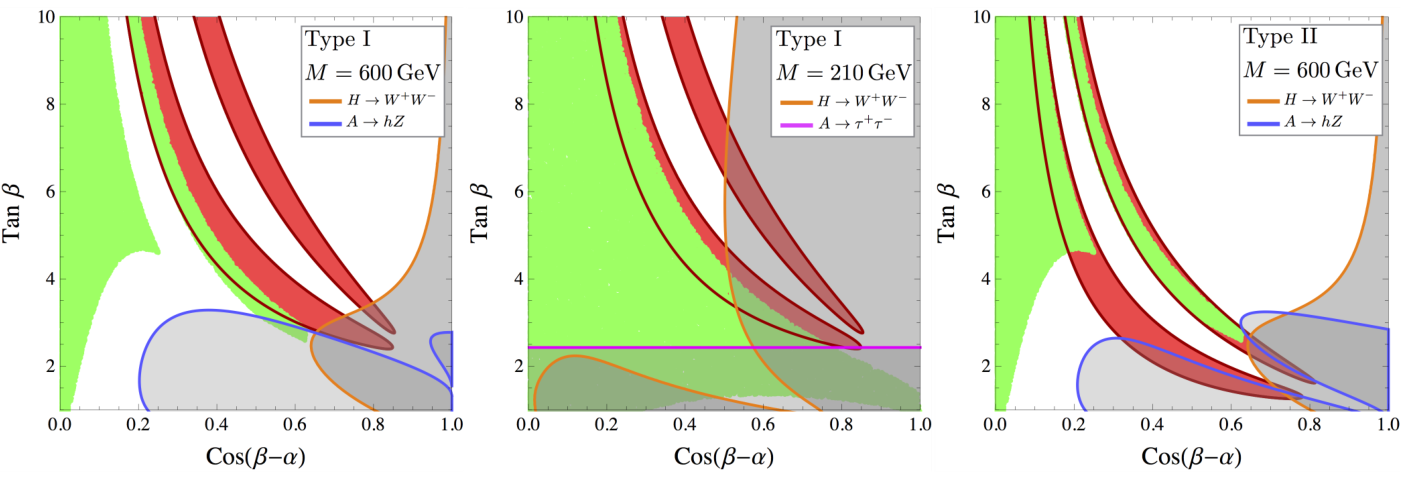In Fig. 2, we show in green the regions allowed by all the above constraints for the type I 2HDFM and $M=600$ GeV ($M=210$ GeV) in the left (center) panel, as well as for type II 2HDFM and $M=600$ GeV in the right panel. Fig. 2 includes perturbativity and unitarity conditions, as well as bounds from electroweak precision measurements (EWPM) at the $2\sigma$ level, based on the Two-Higgs-Doublet Model Calculator [9] and the values provided by the Gfitter analysis [10].

References

- [1] C. Froggatt and H. B. Nielsen, Nucl.Phys. B147, 277 (1979).
- [2] K. Babu and S. Nandi, Phys.Rev. D62, 033002 (2000), arXiv:hep-ph/9907213 [hep-ph] .
- [3] G. F. Giudice and O. Lebedev, Phys.Lett. B665, 79 (2008), arXiv:0804.1753 [hep-ph] .
- [4] M. Bauer, M. Carena, and K. Gemmler, JHEP 11, 016 (2015), arXiv:1506.01719 [hep-ph] .
- [5] G. Branco, P. Ferreira, L. Lavoura, M. Rebelo, M. Sher, et al., Phys.Rept. 516, 1 (2012), arXiv:1106.0034 [hep-ph] .
- [6] M. Bona et al. (UTfit), JHEP 0803, 049 (2008), Updates available on http://www.utfit.org., arXiv:0707.0636 [hep-ph] .
- [7] V. Khachatryan et al. (CMS), JHEP 1410, 160 (2014), arXiv:1408.3316 [hep-ex] .
- [8] M. Misiak et al., Phys. Rev. Lett. 114, 221801 (2015), arXiv:1503.01789 [hep-ph] .
- [9] D. Eriksson, J. Rathsman, and O. Stal, Comput.Phys.Commun. 181, 189 (2010), arXiv:0902.0851 [hep-ph] .
- [10] M. Baak et al. (Gfitter Group), Eur.Phys.J. C74, 3046 (2014), arXiv:1407.3792 [hep-ph] .
- [11] ATLAS-CONF-2015-007 (2015).
- [12] Scalar: CMS Run 1 final results, prospectives for Run 2 (and HL-LHC), talk by Josh Bendavid at the 50th Rencontres de Moriond EW 2015.
- [13] M. Spira, (1995), arXiv:hep-ph/9510347 [hep-ph] .
- [14] S. Dittmaier et al. (LHC Higgs Cross Section Working Group), (2011), 10.5170/CERN-2011-002, arXiv:1101.0593 [hep-ph] .
- [15] S. Heinemeyer et al. (LHC Higgs Cross Section Working Group), (2013), 10.5170/CERN-2013-004, arXiv:1307.1347 [hep-ph] .
- [16] A. Djouadi, J. Kalinowski, and P. Zerwas, Z.Phys. C70, 435 (1996), arXiv:hep-ph/9511342 [hep-ph] .
- [17] V. Khachatryan et al. (CMS), (2015a), arXiv:1504.00936 [hep-ex] .
- [18] V. Khachatryan et al. (CMS), (2015b), arXiv:1504.04710 [hep-ex] .
- [19] G. Aad et al. (ATLAS), Phys.Lett. B744, 163 (2015), arXiv:1502.04478 [hep-ex] .
- [20] CMS-PAS-HIG-13-022 (2013).