Measuring the Higgs-bottom coupling in weak boson fusion
Abstract
We study Higgs production through weak boson fusion with subsequent decay to bottom quarks. By combining jet substructure techniques and matrix element methods in different limits we motivate this channel as a probe of the bottom-Yukawa interactions in the boosted regime. In particular we ameliorate the “no-go” results of cut-and-count analyses in this channel. After applying a data-driven reconstruction approach we find that the Higgs-bottom coupling can be limited to with .
I Introduction
After the Higgs discovery [1, 2] and a growing consistency of Higgs measurements by ATLAS and CMS with the Standard Model (SM) hypothesis [3], diversifying and extending Higgs to all available production and decay channels is of utmost importance. On the one hand, this strategy will us allow to over-constrain fits to, e.g., the dimension six extension of the Higgs sector, or, on the other hand, could facilitate a new physics discovery in non-standard and less “traditional” Higgs search channels.
The coupling of the Higgs boson to bottom quarks is outstandingly important in this regard, because we expect a Higgs decay to bottom final states at around 60% [4]. Yet, none of the currently available analyses is directly sensitive to this coupling. Even the smallest deviation of the Higgs coupling to bottom quarks has far reaching consequences for the Higgs lifetime; a modification of which might, e.g., point to a possible relation of the TeV scale with a hidden sector. Since a modified Higgs phenomenology can arise from multiple sources, fingerprinting the bottom Yukawa interaction is mandatory to experimentally verify mass generation of the third generation down sector, especially because the standard ways of looking for Yukawa interactions such as Higgs production or bottom-quark associated Higgs production suffer either from dominant virtual top-quark contributions or a small total rate in light of a huge background.
In fact, there are only a few processes that contribute to a direct measurement of the bottom-Yukawa coupling: associated Higgs production [5, 6, 7] and top-associated Higgs production [8, 9, 10], with subsequent decay , both of which are challenging to probe at the LHC, even with large statistics.
It is the purpose of this work to add another sensitive channel to this list: weak boson fusion (WBF)-like Higgs production with decay to bottom quarks. This channel has been studied in Ref. [11], which quoted a very small signal vs. background ratio, effectively removing this process from the list of interesting Higgs processes. This is mainly due to large backgrounds and little handle (such as a missing central jet veto [12, 13, 14]) to control them. In this work we extend the analysis of [11] by employing novel reconstruction and all-information approaches through combining shower deconstruction [15, 16], an all-order matrix element method to analyse fat jets, with the fix-order matrix element method techniques [17, 18] for the hard process. We show that the large backgrounds can be significantly reduced, while a major part of the signal can be retained. This allows us to ameliorate the no-go expectation of “traditional” cut-and-count analyses for WBF Higgs production with -quark final states.
This work is organised as follows. In Sec. II, we comment on our event generation and the used analysis tools. Specifically, we review the matrix element method and shower deconstruction in Secs. II.2 and II.3 to make this work self-contained. Sec. III is devoted to our results. We perform a naive cut-and-count analysis and show that kinematic handles alone do not provide enough discriminating power to sufficiently isolate signal from background. We show that the latter can be achieved with a combination of matrix element method and shower deconstruction techniques, leading to an expected sensitivity to the SM WBF contribution with around luminosity. Sec. IV provides a summary and gives our conclusions.
II Event generation and analysis tools
II.1 Event generation
We generated events at Leading Order in the four flavor scheme with MadGraph5_aMC@NLO [19, 20, 21]/Pythia8.2 [22] using NNPDF2.3 [23] for the parton distribution functions. The generation was split into five independent samples: two for the signal and three for the background. The two signal samples are the Higgs production in association with two light jets via either weak boson fusion (WBF) or via gluon fusion (GF) with the Higgs decaying into a pair. The gluon fusion process was generated via the new extension of MadGraph5_aMC@NLO supporting loop induced processes [24] and includes the full top and bottom mass effects. For the background we split the final state into pure QCD production (referred to as ) and electroweak production (referred to as ). The last background sample is the four light-flavor jet sample (), for which we limit ourselves to the pure QCD contribution. To avoid the double counting between the and the samples related to emission in the parton-shower, we ran a four flavor parton-shower for the sample.
At parton level a couple of loose cuts are applied in order to gain in efficiency. For all the samples with two quarks and two light jets in the final state, we apply the following cuts:
For the sample, the same cuts are applied with the index “” being identified as the two most forward jets and the index “” refers to the two central jets.
II.2 The Matrix Element method
The matrix element method [17, 18] is based on the Neyman-Person Lemma [25] stating that the best discriminant variable is the likelihood ratio where the likelihood is the product of probabilities evaluated on the sample. The probability of an event is computed in the matrix element method by calculating
where represents the measured momenta for a given event, is the partonic phase-space point which we integrate over with a phase-space measure that also includes the parton distribution functions. is the matrix element square for a given hypothesis and , named the transfer functions, is the conditional probability to observe the experimental event under consideration for a given partonic phase-space point.
Using the best discriminant variable allows us to perform measurements for processes with extremely small cross-section or small event rate. However, even if the above integral can be computed via dedicated tools [26], this is very CPU intensive when performed for the full sample of events. In order to analyse large background samples efficiently, we therefore simplify the method by approximating the transfer function by a delta function, allowing us to drop the computation of the integral entirely [15, 27]. This is conservative, since including such effect can only improve the sensitivity of the method** * Further improvements could be achieved by evaluating the matrix elements at NLO accuracy [28, 29]..
Therefore, for each event, the matrix element method is equivalent to computing the following likelihood ratio:
| (1) |
For additional speed efficiency, the gluon fusion matrix element is not computed using the one loop matrix element – like we did for the event generation – but at tree level with an effective vertex coming for the integrating out the top quark loop [30]. The signal matrix elements ( and ) are computed for a three body final state (with the Higgs momentum being identified with the reconstructed -pair momentum) while the backgrounds are computed for the four particle final state using the tagged subjet from the fat jet (see Sec. III). To avoid potential bias, we use different sets of PDFs for the analysis (CT10 [31]) compared to the one used for the event generation.
II.3 Shower Deconstruction
Shower deconstruction [15, 16] is an all-order matrix element method designed to discriminate hadronically decaying electroweak-scale resonances, i.e. tops, or Higgs boson, from QCD jets. First the constituents of a fatjet are reclustered into small inclusive jets, e.g. using the jet algorithm [32] with R=0.2 and GeV. One obtains a configuration of subjets with four-momenta . Using these subjets as input to the method, a likelihood ratio is calculated from first-principle QCD, quantifying whether the observed distribution of subjets was initiated by the decay of a signal process, e.g. a Higgs boson, or background, e.g. a gluon. To calculate the likelihood ratio
| (2) |
where represents the probability of obtaining the subjet distribution given the signal hypothesis, and is the probability for obtaining the same from background processes. To calculate and the method sums over all possible shower histories. In [33] it was shown that is insensitive to pileup and shows good agreement between data and Monte-Carlo prediction. We follow loosely the approach described in [34] to combine shower deconstruction with the fix-order matrix element method of Sec. II.2.
III Results
Based on the event generation detailed above, we first establish a baseline cut scenario inspired by [11, 35].


| WBF | GF | |||||
|---|---|---|---|---|---|---|
| (i) | fat jet | 48.50 | 17.32 | 205109 | 553.16 | |
| (ii) | wbf cuts | 21.23 | 4.11 | 48441.9 | 127.98 | |
| (iii) | mercedes star | 18.44 | 2.82 | 31674.5 | 84.975 | |
| (iv) | fatjet -tags | 4.59 | 0.578 | 3800.99 | 12.57 | 323.74 |
In the first step, we veto events with isolated leptons with and GeV. We then request a Cambridge-Aachen [36] fat jet†† † Jet finding and clustering is performed with FastJet [37]. with
| (3) | ||||
After having identified a fat jet, we remove its constituents from the final state, and the remaining constituents in the event are clustered using anti-kT jets [38] with GeV in . The two jets with largest rapidity we define as so-called tagging jets and .
In the next step, we impose typical and stringent WBF selection requirements on these two tagging jets; they need to have a large invariant mass, are required to lie in different detector hemispheres, and need to be separated by a large rapidity gap
| (4) | ||||
The first cut in particular decreases the gluon fusion contribution significantly which is a necessary requirement to end up with the clean WBF-like selection to separate the impact of new physics between the two production modes [27].
The typical WBF event topology that we want to isolate is a Mercedes star configuration. Hence, we veto events for which one of the tagging jets is central or collimated to the fat jet, i.e. we require
| (5) |
in the third step of the analysis.


Since the fat jet is produced centrally, we cannot use generic ways to reduce the hadronic backgrounds, such as central/mini-jet vetos which would also push the gluon fusion contribution to the percent level.
In the last step, we turn to the fat jet that we removed earlier from the event record. We recombine the constituents of the fat jet to so-called microjets with and GeV. Of these microjets we require the two with largest transverse momentum to be -tagged. We assume a flat tagging efficiency and fake rate. To facilitate a -tag, the microjets need to have GeV. We decay the -mesons, do not account for missing energy in the reconstruction (hence our result is conservative), and, in addition to the assumed tagging efficiency, for a -tag we match the -meson to the respective jet by requiring .
A cut flow of our analysis is shown in Tab. 1; distributions of signal and backgrounds are shown in Fig. 1. It is important to realise that after step (iii) we have exhausted all kinematic handles to suppress the backgrounds and find ourselves in the unfortunate situation that -tagging is not discriminative enough to cure a bad signal vs. background ratio.‡‡ ‡ We have checked that the top pair background also contributes at this stage, but becomes completely negligible in the matrix element method+shower deconstruction signal region detailed below. Increasing the invariant mass cut would lead to a further suppression of the backgrounds, however at an unacceptably large decrease of the signal yield, leading to a vanishing sensitivity to WBF.§§ § Our results in this regard are compatible with the earlier results of Ref. [11].
With all “traditional” means exhausted we are left with two approaches: (i) reverting to multivariate techniques such as boosted decision trees or neural networks which heavily rely on the treatment of systematics and training, combining a few observables that still show promise to increase signal over background (see e.g. the recent Ref. [40]), or (ii) improve the analysis in a way that is motivated by the asked physics question. The latter avenue is exactly provided by combining the matrix element method for the hard process with shower deconstruction, a matrix element method for soft and collinear QCD radiation. The former provides a statistical discrimination on the basis of expected signal and background contributions, while the latter isolates the decay from the irreducible backgrounds by comparing the different shower histories.
We separately calculate of Eq. (2) and of Eq. (1), see Fig. 2. Again, this approach is conservative, as the sensitivity of the analysis can be increased by combining shower deconstruction and the matrix element method, see [34] for a discussion. The two-dimensional correlation of matrix element method and shower deconstruction isolates a region of phase-space with a maximum signal-over-background ratio of , requiring at least 3 signal events in isolated bins at 100/fb. Since shower deconstruction can highly discriminate between and the continuum background, by integrating over adjacent bins in the shower deconstruction observable, we obtain this way 10 events for 100/fb at a reduced signal vs. background ratio of . While this constitutes a tremendous improvement over the cut and count analysis with , it is still obvious that background systematics can have a significant impact.
Since this would render a likelihood analysis of the matrix element method-shower deconstruction correlation unreliable, we instead turn to a data driven approach based on pre-selecting a matrix element likelihood regime favored by the signal and fitting the background distribution of the shower deconstruction output. In practice, a fit based on a product of a Gaussian and a polynomial of degree 2
| (6) |
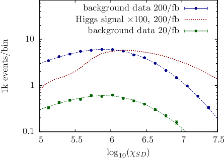
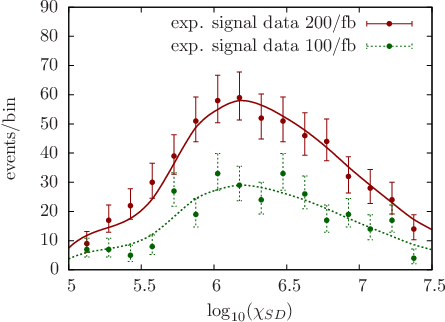
with fitted parameters works very well as the background template with , see Fig. 3. This opens the possibility to perform a search for the Higgs boson similarly to the search for the Higgs in other channels under the conditions that the background is not very well understood, leading to large systematics once theoretical uncertainties are treated at face value: one uses a background fit function that is motivated from MC analysis to fit the distribution, which then has small systematic uncertainty and looks for enhancements over the expected background model. With increased statistics the fit quality becomes better and systematic uncertainties become negligible quickly (again similar to the situation in searches). Concretely we find the signal to be clustered around while the background distribution is a smooth Gaussian-like distribution of Eq. (6) in the search region .
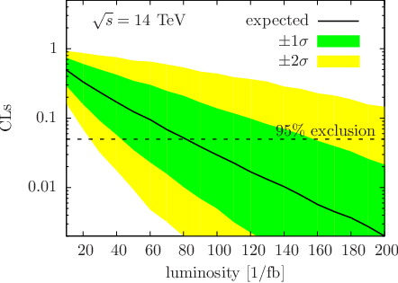
At a luminosity fb the total number of signal events, as well as the different shape of the signal distribution, Figs. 3 and 4, becomes resolvable on the basis of the binned log likelihood method of [42, 39] (we stress again that the error bars in Figs. 3 and 4 are purely exemplary; the correct combined background+signal distributions are sampled in using the methods of [42, 39] and taken into account in the limits we quote). This means we can start excluding the SM at 95% confidence level in case the Higgs has a suppressed bottom Yukawa interaction, Fig. 5. On the other hand, assuming a SM-like Higgs boson, we can turn this exclusion into a coupling measurement. Projecting to , we obtain a constraint
at 95% confidence level by propagating the impact of the modified bottom Yukawa interaction through the Higgs production and decay phenomenology while keeping all other Higgs couplings fixed to their SM values.
IV Summary and Conclusions
In this paper we have performed an analysis of Higgs production via weak boson fusion (WBF) with subsequent decays . While this process is heavily plagued with backgrounds due to the non-availability of signal vs. background enhancing strategies like the central jet veto, we have shown that by combining novel analysis strategies, we can elevate the discouraging result of a simple cut-and-count analysis that exploits the basic kinematic features of WBF to a sensitive strategy at a luminosity of about . Our strategy has the additional advantage that it relies on a data-driven fit of the background template, which is derived from first principle QCD and fixed-order calculations instead of relying on nontransparent multivariate techniques. Crucial to this strategy is that the matrix element method and shower deconstruction combine complementary information - an analysis solely based on one of these tools does not provide enough discriminating power to increase the sensitivity to WBF Higgs production in the bottom final state. As a result, during the upcoming run of the LHC, ATLAS and CMS will be able to probe the Higgs-bottom coupling in a complementary way to well established measurements in and .
Acknowledgements.
M.S. acknowledges financial support by HiggsTools ITN under grant agreement PITN-GA-2012-316704. O.M. is a Durham International Junior Research Fellow.References
- [1] G. Aad et al. [ATLAS Collaboration], Phys. Lett. B 716 (2012) 1.
- [2] S. Chatrchyan et al. [CMS Collaboration], Phys. Lett. B 716 (2012) 30 [arXiv:1207.7235 [hep-ex]].
- [3] F. Englert and R. Brout, Phys. Rev. Lett. 13 (1964) 321. P. W. Higgs, Phys. Lett. 12 (1964) 132 and Phys. Rev. Lett. 13 (1964) 508. G. S. Guralnik, C. R. Hagen and T. W. B. Kibble, Phys. Rev. Lett. 13 (1964) 585.
- [4] S. Dittmaier et al. [LHC Higgs Cross Section Working Group Collaboration], arXiv:1101.0593 [hep-ph].
- [5] J. M. Butterworth, A. R. Davison, M. Rubin and G. P. Salam, Phys. Rev. Lett. 100, 242001 (2008) doi:10.1103/PhysRevLett.100.242001 [arXiv:0802.2470 [hep-ph]].
- [6] D. E. Soper and M. Spannowsky, JHEP 1008, 029 (2010) doi:10.1007/JHEP08(2010)029 [arXiv:1005.0417 [hep-ph]].
- [7] J. M. Butterworth, I. Ochoa and T. Scanlon, Eur. Phys. J. C 75, no. 8, 366 (2015) doi:10.1140/epjc/s10052-015-3592-5 [arXiv:1506.04973 [hep-ph]].
- [8] T. Plehn, G. P. Salam and M. Spannowsky, Phys. Rev. Lett. 104, 111801 (2010) doi:10.1103/PhysRevLett.104.111801 [arXiv:0910.5472 [hep-ph]].
- [9] P. Artoisenet, P. de Aquino, F. Maltoni and O. Mattelaer, Phys. Rev. Lett. 111, no. 9, 091802 (2013) doi:10.1103/PhysRevLett.111.091802 [arXiv:1304.6414 [hep-ph]].
- [10] N. Moretti, P. Petrov, S. Pozzorini and M. Spannowsky, arXiv:1510.08468 [hep-ph].
- [11] M. L. Mangano, M. Moretti, F. Piccinini, R. Pittau and A. D. Polosa, Phys. Lett. B 556 (2003) 50 [hep-ph/0210261].
- [12] Y. Dokshitzer, V. Khoze, and S. Troyan, in M. Derrick (ed.), “Physics In Collision 6. Proceedings, 6th International Conference, Chicago, USA, September 3-5, 1986,” Singapore, Singapore: World Scientific (1987) 542 p.
- [13] J. D. Bjorken, Int. J. Mod. Phys. A 7 (1992) 4189. J. D. Bjorken, Phys. Rev. D 47 (1993) 101.
- [14] U. Baur and E. W. N. Glover, Phys. Lett. B 252 (1990) 683. V. D. Barger, K. -m. Cheung, T. Han and D. Zeppenfeld, Phys. Rev. D 44 (1991) 2701 [Erratum-ibid. D 48 (1993) 5444]. D. L. Rainwater, R. Szalapski and D. Zeppenfeld, Phys. Rev. D 54 (1996) 6680.
- [15] D. E. Soper and M. Spannowsky, Phys. Rev. D 84, 074002 (2011) doi:10.1103/PhysRevD.84.074002 [arXiv:1102.3480 [hep-ph]].
- [16] D. E. Soper and M. Spannowsky, Phys. Rev. D 87, 054012 (2013) doi:10.1103/PhysRevD.87.054012 [arXiv:1211.3140 [hep-ph]].
- [17] K. Kondo, J. Phys. Soc. Jap. 57, 4126 (1988). doi:10.1143/JPSJ.57.4126
- [18] V. M. Abazov et al. [D0 Collaboration], Nature 429, 638 (2004) doi:10.1038/nature02589 [hep-ex/0406031].
- [19] J. Alwall et al., JHEP 1407, 079 (2014) doi:10.1007/JHEP07(2014)079 [arXiv:1405.0301 [hep-ph]].
- [20] C. Degrande, C. Duhr, B. Fuks, D. Grellscheid, O. Mattelaer and T. Reiter, Comput. Phys. Commun. 183, 1201 (2012) doi:10.1016/j.cpc.2012.01.022 [arXiv:1108.2040 [hep-ph]].
- [21] P. de Aquino, W. Link, F. Maltoni, O. Mattelaer and T. Stelzer, Comput. Phys. Commun. 183, 2254 (2012) doi:10.1016/j.cpc.2012.05.004 [arXiv:1108.2041 [hep-ph]].
- [22] T. Sjstrand et al., Comput. Phys. Commun. 191, 159 (2015) doi:10.1016/j.cpc.2015.01.024 [arXiv:1410.3012 [hep-ph]].
- [23] R. D. Ball et al., Nucl. Phys. B 867, 244 (2013) doi:10.1016/j.nuclphysb.2012.10.003 [arXiv:1207.1303 [hep-ph]].
- [24] V. Hirschi and O. Mattelaer, JHEP 1510, 146 (2015) doi:10.1007/JHEP10(2015)146 [arXiv:1507.00020 [hep-ph]].
- [25] Neyman, Jerzy; Pearson, Egon S. Philosophical Transactions of the Royal Society A: Mathematical, Physical and Engineering Sciences 231 (694706): 289337. doi:10.1098/rsta.1933.0009
- [26] P. Artoisenet, V. Lemaitre, F. Maltoni and O. Mattelaer, JHEP 1012, 068 (2010) doi:10.1007/JHEP12(2010)068 [arXiv:1007.3300 [hep-ph]].
- [27] J. R. Andersen, C. Englert and M. Spannowsky, Phys. Rev. D 87 (2013) 1, 015019 [arXiv:1211.3011 [hep-ph]].
- [28] J. M. Campbell, W. T. Giele and C. Williams, arXiv:1205.3434 [hep-ph].
- [29] T. Martini and P. Uwer, JHEP 1509 (2015) 083 doi:10.1007/JHEP09(2015)083 [arXiv:1506.08798 [hep-ph]]. T. Martini and P. Uwer, Acta Physica Polonica B . Nov2015, Vol. 46 Issue 11, p2143-2148 doi:10.5506/APhysPolB.46.2143 [arXiv:1511.07150 [hep-ph]].
- [30] J. Alwall et al., JHEP 0709, 028 (2007) doi:10.1088/1126-6708/2007/09/028 [arXiv:0706.2334 [hep-ph]].
- [31] M. Guzzi, P. Nadolsky, E. Berger, H. L. Lai, F. Olness and C.-P. Yuan, arXiv:1101.0561 [hep-ph].
- [32] S. D. Ellis and D. E. Soper, Phys. Rev. D 48, 3160 (1993) doi:10.1103/PhysRevD.48.3160 [hep-ph/9305266].
- [33] The ATLAS collaboration [ATLAS Collaboration], ATLAS-CONF-2014-003.
- [34] D. E. Soper and M. Spannowsky, Phys. Rev. D 89, no. 9, 094005 (2014) doi:10.1103/PhysRevD.89.094005 [arXiv:1402.1189 [hep-ph]].
- [35] V. A. Khoze, W. J. Stirling and P. H. Williams, Eur. Phys. J. C 31, 91 (2003) doi:10.1140/epjc/s2003-01328-8 [hep-ph/0307292].
- [36] Y. L. Dokshitzer, G. D. Leder, S. Moretti and B. R. Webber, JHEP 9708 (1997) 001 [hep-ph/9707323].
- [37] M. Cacciari, G. P. Salam and G. Soyez, Eur. Phys. J. C 72 (2012) 1896 [arXiv:1111.6097 [hep-ph]].
- [38] M. Cacciari, G. P. Salam and G. Soyez, JHEP 0804 (2008) 063 [arXiv:0802.1189 [hep-ph]].
- [39] A. L. Read, J. Phys. G 28 (2002) 2693. doi:10.1088/0954-3899/28/10/313
- [40] V. Khachatryan et al. [CMS Collaboration], Phys. Rev. D 92 (2015) 3, 032008 doi:10.1103/PhysRevD.92.032008 [arXiv:1506.01010 [hep-ex]].
- [41] G. Cowan, “Burning Issues for the Statistics Forum”, presentation at ATLAS Statistics Forum, 5 October, 2010
- [42] T. Junk, Nucl. Instrum. Meth. A 434 (1999) 435 [arXiv:hep-ex/9902006]. T. Junk, CDF Note 8128 [cdf/doc/statistics/public/8128]. T. Junk, CDF Note 7904 [cdf/doc/statistics/public/7904]. H. Hu and J. Nielsen, in 1st Workshop on Confidence Limits, CERN 2000-005 (2000) [arXiv:physics/9906010].