Active processes make mixed lipid membranes either flat or crumpled

Cell membranes are generally made of several lipids and have complex structures [1]. The dynamics of cell membranes are affected by biological active (nonequilibrium) processes (e.g., nonequilibrium fluctuations of cell cytoskeletons [2] and active proteins in the lipid membrane [3]); see also Ref. [4]. Miscibility phase transitions (MPTs) in equilibrium heterogeneous or mixed model lipid bilayers and giant plasma membrane vesicles (GPMVs) are well studied [5, 6]. In contrast, occurrence of MPTs in eukaryotic cell membranes, remains controversial till date [7]. Whether cellular active processes can control membrane fluctuations and associated MPTs in mixed membranes and if so, how, form general motivations for the present study.

Structural and dynamical complexities of cell membranes preclude simple physical understanding of MPTs in cell biological context. This calls for studying this question within a simpler nonequilibrium model appropriate for an in-vitro setting, where this issue may be addressed systematically and possibly verified in suitably designed in-vitro experiments. To this end, in this article we construct a hydrodynamic theory for planar active mixed lipid (fluid) membranes [1]. Hydrodynamic approaches have a long history of applications in both equilibrium [9, 8] and nonequilibrium [10, 11] systems and are successful in predicting general physical properties at large scales independent of the microscopic (molecular) details of the systems. In particular, our theory is applicable to a variety of systems, e.g., a lipid bilayer in an orientable active fluid [10] in its isotropic phase [12] or a lipid bilayer with an active component, e.g., active proteins, immersed in a passive fluid [3]. We use it to study the membrane conformation fluctuations and the associated active or nonequilibrium MPTs. Both second order MPT (through critical and tricritical points), and first order MPT are considered. We uncover a direct correspondence between membrane fluctuations and the nature of the MPTs, potentially opening up a new experimental route to study the MPTs. Our predictions are quite general; we expect that our characterisations of the membrane fluctuations and MPTs should serve as references for experimental observations on MPTs in mixed model lipid bilayers and GPMVs in isotropic actomyosin extracts with adenosine triphosphate (ATP) molecules or solutions of live orientable bacteria [13], and lipid membranes with active protein inclusions embedded in passive fluids. From perspectives of nonequilibrium physics, our model provides an intriguing example where the same underlying microscopic active processes control two distinct phenomena, viz. MPTs of the membrane composition and the nature of fluctuations of the membrane conformation, ultimately linking the two in a definitive way.

In order to focus on the essential physics of the problem, we consider a planar, tensionless, two-component, inversion-symmetric [14], single-layered lipid membrane [15] of linear size $L$. In stark contrast to equilibrium lipid membranes [16, 17], our model membrane displays generic stiffening and statistical flatness for positive active tensions $\sigma_{a}$, but softening and crumpling for $\sigma_{a}<0$ at any temperature $T$. We describe the planar membrane conformations by a single-valued height field $h({\bf x},t)$ in the Monge gauge [18, 9], in two dimensions ($2d$) with the local normal ${\bf n}=(-{\boldsymbol{\nabla}}h,1)=({\delta\bf n},1)$ [18, 9]. Then, for positive $\sigma_{a}$, away from the critical point for second order MPT and across first order MPT we find variances

in the thermodynamic limit (TL). These imply orientational long range order (LRO), hence statistical flatness and positional quasi long range order (QLRO); here $\langle..\rangle$ implies averaging over noises; see dynamical equations (8) and (9), respectively, below. Near the critical point, the membrane becomes super stiff: in a mean-field like treatment, we show

in TL, an $L$-dependence weaker than in QLRO, which we call positional nearly long range order (NLO). Moreover, $\Delta_{n}$ is further suppressed near the critical point. In contrast, for $\sigma_{a}<0$, $\Delta_{n}$ and $\Delta_{h}$ diverge for membranes larger than a persistence length, i.e., $L>\zeta$ [17], indicating orientational and positional short range orders (SRO). The rest of this article is organised as follows. In Sec. II, we set up our coarse-grained equations of motion. Then in Sec. III we discuss our results on the membrane conformation fluctuations at or across various MPTs. Section IV discusses the various MPTs possible within our model. Finally, in Sec. V we summarise our results. A glossary of our results has been added in Sec. VI for the convenience of the readers. Some technical aspects of the calculations involved and a few additional discussions related to the main results of this work are made available in Appendices A to G for interested readers.

We consider an incompressible mixed permeable membrane composed of two lipids A and B of equal amount with local concentrations $n_{A}({\bf x},t)$ and $n_{B}({\bf x},t)$, respectively [17], $n_{A}+n_{B}=1$. The local inhomogeneity $\phi~(=n_{A}-n_{B}$) is the order parameter for the MPT. Since the active processes may in general interact differently with A and B, we relax the usual inversion symmetry of $\phi$ for a binary mixture [19] when coupled to local mean curvatures in the present model (see Refs. [17, 20, 21] in this context).

Now, consider a nearly flat permeable membrane spread parallel to the $xy$-plane, i.e., with local normals parallel to the $z$-axis on average; see Fig. 1 for a schematic diagram.

While the height field $h$ is a nonconserved broken symmetry variable, the order parameter field $\phi$ is a conserved density, since $n_{A}$ and $n_{B}$ are conserved. The relevant equations of motion for $h$ and $\phi$ may be derived as follows. The membrane, treated as a permeable fluid film [22], has a local velocity in the normal direction (along $z$ direction in this case) $v_{mz}$ given by

Here, $v_{hydro_{z}}$ is the $z$-component of the local three-dimensional ($3d$) hydrodynamic velocity ${\bf v}_{hydro}$ [12], and $v_{perm}$ represents the local permeative flows [12]. In general, both $v_{perm}$ and ${\bf v}_{hydro_{z}}$ may contain equilibrium (controlled by a free energy $\mathcal{F}$; see below) and active parts. The latter contributions cannot be obtained from $\mathcal{F}$. Instead, symmetry considerations (e.g., translation, in-plane rotation, inversion symmetry of $h$ and invariance under tilt for the membrane) may be used to enforce the general forms of the active contribution to $v_{perm}$. We write

to the lowest order in nonlinearities and gradients satisfying the relevant invariances. The first term on the rhs of (5) with coefficients $\lambda$ and $\tilde{\lambda}$ is the active contribution to $v_{perm}$; $\mu_{p}$ is a (constant) kinetic coefficient for the equilibrium contribution to the permeative flows. The active terms with coefficients $\lambda$ and $\tilde{\lambda}$ are forbidden in equilibrium due to the tilt invariance of the associated free energy $\mathcal{F}$ (see below)  [17]. They are, however, permitted here as the tilt invariance in the present problem must hold at the level of the equations of motion [11]. All of $\lambda,\tilde{\lambda},\mu_{p}$ vanish for impermeable membranes. Furthermore, $\lambda$ and $\tilde{\lambda}$ control the strength of $\sigma_{a}$, the active tension (see below); a non-zero $\tilde{\lambda}$ models the asymmetric dependence of the active processes on lipids A and B. Symmetry arguments cannot determine the signs of $\lambda,\tilde{\lambda}$. In this work, we examine the consequences of both positive and negative $\lambda$; the sign of $\tilde{\lambda}$ can be absorbed within the definition of $\phi$. Further, for a membrane with a fixed background there are no active contributions to $v_{hydro_{z}}$ that are more relevant than the $\lambda,\tilde{\lambda}$-terms above [23]; $v_{hydro_{z}}=-\Gamma_{0}\delta{\mathcal{F}}/\delta h$ with kinetic coefficient $\Gamma_{0}$ being a constant. The dynamics of $\phi$ should generally follow a conservation law form advection-diffusion equation [8]. To proceed further, we assume $\mathcal{F}$ for a tensionless, mixed lipid membrane to have the simple generic form

Here $r=T-T_{c}$, $u,v>0$. Couplings $g$ and $\tilde{h}$ can be of either sign; for a symmetric binary mixture $g=0=\tilde{h}$. Coupling $v$ has been added for reasons of thermodynamic stability (see below) and is irrelevant in equilibrium with $u>0$. Free energy (6) without membrane fluctuations ($h=const.$) describes MPTs identical to the standard liquid-gas phase transition that is generally first order in nature, and admits a second order MPT at a critical point that can be accessed only by setting $T=T_{c}$ and also tuning $\tilde{h}$ to a critical value (equivalently setting pressure $p=p_{c}$, the critical pressure), in analogy with magnetic systems [9]. This analogy can be made more precise by expanding $\mathcal{F}$ about $\phi=\phi_{0}$, with $\phi_{0}$ is chosen such that the $g\phi^{3}$-term in $\mathcal{F}$ above vanishes. The resulting transformed free energy has the form same as that of the Ising model at a finite external magnetic field $\tilde{h}_{0}$ (related to $\tilde{h}$ and depends upon the chemical potential and temperature) that has generic first order MPTs (or may show no transitions) if $\tilde{h}_{0}$ is tuned at any general $T$; furthermore, second order MPT belonging to the $2d$ Ising universality class is found if both $T$ and $\tilde{h}_{0}$ are tuned; the corresponding critical point is located in a $T-\tilde{h}_{0}$-plane at $r=0$ or $T=T_{c}$ (in a mean-field description) and $\tilde{h}_{0}=0$ [9]. In fact, the path in the temperature - pressure plane of a binary mixture that directly resembles the zero magnetic field path in a magnet (which shows a second order transition) is the one with the density fixed at the critical density, i.e., the critical isochore. Notice that the coexistence curve for $\mathcal{F}$ above is similar to that for the Ising model, except now being asymmetric with respect to the order parameter $\langle\phi\rangle=m$ due to the lack of any symmetry of $\mathcal{F}$ under inversion of $\phi$ [9]. The inclusion of $h$-fluctuations in (6) via the couplings $\lambda_{1},\lambda_{2}$ does not alter this picture [6, 17]. This may be easily seen from the form of $\mathcal{F}$: the $\lambda_{1}$ and $\lambda_{2}$ terms effectively only induce fluctuation-corrections to $r$ and $\tilde{h}$, respectively. To what degree this equilibrium physical picture is affected by the activity remains to be seen (see below).

Notice that $\mathcal{F}$ implies an effective composition-dependent bending modulus $\tilde{\kappa}(\phi)$ of the form [17]

Parameters $\lambda_{1},\lambda_{2}$ should be chosen to ensure $\tilde{\kappa}(\phi)>0$ for all $\phi$, that guarantees a thermodynamically stable flat phase, given by the minimum of $\mathcal{F}$, in equilibrium. We choose $\lambda_{1}>0$ [17]. The sign of $\lambda_{2}$ is arbitrary and can be absorbed within the definition of $\phi$; for concreteness we choose $\lambda_{2}>0$. While the individual signs of $\tilde{\lambda}$ and $\lambda_{2}$ are arbitrary, the sign of the product $\lambda_{p}\equiv\tilde{\lambda}\lambda_{2}$ is crucial to what follows below and controls the ensuing macroscopic behaviour.

Putting together everything, the dynamical equations for $h$ (with $\partial_{t}h=v_{mz}$) and $\phi$ to the lowest order in spatial gradient expansions, in the long wavelength limit take the forms (for a fixed background medium)

Notice that the terms with coefficients $\lambda_{1},\lambda_{2}$ in (6) generate additional equilibrium terms in (8); these are however subleading in the hydrodynamic limit (in a scaling sense) to the active $\lambda,\tilde{\lambda}$-terms, respectively, and are hence omitted from (8) [25]. Kinetic coefficient $\Gamma_{h}=\mu_{p}+\Gamma_{0}$ is a constant for a membrane with a fixed background; $\Gamma_{\phi}$ is also a constant. Notice that separately Eq. (9) may be wholly obtained from $\mathcal{F}$ and is just of the “model B” conservation law form (in the nomenclature of Ref. [8]); this is because there are no active terms which are more relevant (in a scaling sense) than those already included in (9). In fact, the $\lambda_{1}-$ and $\lambda_{2}-$ nonlinear terms in (9) originate from the composition-dependent bending modulus $\kappa(\phi)$ in (7) in the free energy (6). This does not, however, in general imply that $\phi$ follows an equilibrium dynamics; its coupling with $h$ ensures that the resulting effective dynamics for $\phi$ is detailed balance breaking. Further, we have ignored any in-plane advection of $\phi$ for simplicity [26]. Noises $f_{h}$ and ${\bf f}_{\phi}$ are zero-mean, Gaussian distributed with variances given by

Here, $D_{h}\neq D_{\phi}$ in general; ${\bf q,q}^{\prime}$ are wavevectors and $\omega,\omega^{\prime}$ are frequencies, $q=|\bf q|$. Noises $f_{h}$ and $f_{\phi i}$ should contain both thermal as well as active contributions.

In this Sec. we first derive our results on membrane fluctuations without any (equilibrium) surface tension by using the model equation (8). We analyse Eq. (8) in a mean field-like spirit and compare its properties with an isolated tensionless fluid membrane at thermal equilibrium. We then establish their correspondence with the order of MPTs, the principal prediction of this work. Next, we briefly touch upon how a finite surface tension may affect our results. We now proceed to discuss these in details below.

There is no general framework available to study phase transitions in nonequilibrium systems. Nonetheless we are able to analyse the MPTs here by drawing analogy between the effective theory for composition fluctuations and standard equilibrium results.

Regardless of the nature of MPTs, we have for a symmetric membrane $\langle\nabla^{2}h\rangle=C=0$. Now, ignoring height fluctuations, if we substitute $\nabla^{2}h$ by $C=0$ in (9), it reduces to the standard equilibrium, conserved dynamics (model B in the nomenclature of Ref. [8]), corresponding to the free energy (6) [with $h=const.$] that yields phase behaviour identical to the standard liquid gas transition at temperature $D_{\phi}$: phase coexistence for $r<0$ or $T<T_{c}$ with an asymmetric coexistence curve about the critical density and a critical point at $T=T_{c}$ belonging to the $2d$ Ising universality class [9]. Thus any active modification of this equilibrium-like picture should be fluctuation induced. To investigate that further, we follow Ref. [39] and perturbatively integrate out $h$-fluctuations and obtain an effective dynamical equation for $\phi$ only. Operationally, to account for the fluctuation effects at the simplest level, we calculate the effective (fluctuation-corrected) parameters of (9) at the lowest order in perturbative expansions. We then express (9) in terms of the fluctuation-corrected parameters and substitute $\nabla^{2}h$ by $\langle\nabla^{2}h\rangle(=0)$, ignoring fluctuations. In this approximation, the $\phi$-dynamics is entirely described by a fluctuation-corrected free energy $F_{\phi}$, entirely decoupled from $h$ which has the form

with

as the attendant effective dynamical equation for $\phi$. In (32), $u_{e}$ and $g_{e}$ include one loop corrections to the bare couplings $u$ and $g$, respectively. Here we have ignored the corrections to $r$ and $v$ since these are not central to the analysis here; a correction to $r$ merely shifts $T_{c}$ and we assume $v$ is always positive. Further, $\tilde{h}$ has no active corrections at the lowest order. Thus the one-loop effective dynamics of $\phi$ follows the equilibrium model B dynamics with free energy $F_{\phi}$ at an effective temperature $D_{\phi}$.

With $\lambda>0$, retaining only the inhomogeneous active one-loop correction to $u$ and $g$ (this suffices for our arguments here) we obtain $u_{e}=u+\Delta u=u+\lambda_{p}\tilde{\lambda}^{2}D_{h}A$ and $g_{e}=g+\tilde{\lambda}^{2}\lambda_{2}D_{h}B_{1}+\lambda\lambda_{2}D_{h}B_{2}$ where, $\lambda_{p}=\lambda_{2}\tilde{\lambda}$ and $A,B_{1},B_{2}$ are numerical constants; see Appendix C. Thus effective couplings $u_{e}$ and $g_{e}$ can be independently positive, negative or zero.

The phase behaviour and transitions of $\phi$ can be directly obtained from $F_{\phi}$. First consider $u_{e}>0$. The term $v\phi^{6}$ in (32) is now redundant and we ignore it. Then $F_{\phi}$ has the same form as $\mathcal{F}$ in (6). As a result, the discussions that immediately follow $\mathcal{F}$ apply to $F_{\phi}$ as well: by making a suitable shift in $\phi$, the cubic term $g_{e}\phi^{3}$ may be eliminated from $F_{\phi}$, yielding a modified form for $F_{\phi}$ identical to the free energy for the Ising model in the presence of an external magnetic field $\tilde{h}_{\phi}$. Then, composition $\phi$ generally undergoes a first order MPT below a transition temperature. A critical point with a second order MPT may be accessed only by suitable tuning of both $T$ and $\tilde{h}_{\phi}$: in fact the critical point is located in the $(T,\tilde{h}_{\phi})$ plane at $r=0$ or $T=T_{c}$ and $\tilde{h}_{\phi}=0$, with an associated universal scaling behaviour belonging to the $2d$ Ising universality class [9]. Since $\tilde{h}_{\phi}$ in general does depend on the active coefficients $\lambda,\tilde{\lambda}$, tuning activity can make $\tilde{h}_{\phi}=0$. Further, $T_{c}$ too receives fluctuation corrections that depends on activity (not shown here). Thus the critical point for this nonequilibrium second order MPT can be accessed by controlling the activity. The role of $g_{e}\neq 0$ is only to introduce an asymmetry of the order parameter $\langle\phi\rangle=m$ about the critical density, reflected in the curvature of the coexistence curve at the criticality [9]. Since $g_{e}$ can be varied continuously and made positive, negative or zero by tuning the composition-membrane interactions parameters, the curvature at criticality and hence the location of the coexistence curve in the $\phi-D_{\phi}$ plane changes continuously with the active parameters. Experimental measurements of the coexistence curve for a given system can thus reveal valuable quantitative information about the active coefficients and the underlying active processes in the membrane.

To ensure thermodynamic stability for $u_{e}<0$, we need to include the $v\phi^{6}$-term into consideration. This then yields a first order MPT at temperature $T^{*}=T_{c}+2u_{e}^{2}/(3v)$ and $m^{2}=|u_{e}|/(2v)$ even for $\tilde{h}_{\phi}=0$ in direct analogy with the known equilibrium MF results [9]. At the tricritical point, $u_{e}=0$, i.e., $u=-\lambda_{p}\tilde{\lambda}^{2}D_{h}nA$ and $\tilde{h}_{\phi}=0$. Notice that, unlike equilibrium examples of tricritical points [9], here the condition for the tricritical point explicitly involves $D_{h}$, thus bearing the hallmark of nonequilibrium [40]. While the MPTs for $u_{e}>0$ are essentially indistinguishable from their equilibrium counterparts or the equilibrium liquid-gas phase transitions with a second order MPT accessible by setting $\tilde{h}_{\phi}=0$ and tuning $T$ to $T_{c}$, the prospect of a first order MPT for $u_{e}<0$ at $\tilde{h}_{\phi}=0$ at $T=T^{*}>T_{c}$ and the associated tricritical point are truly remarkable in that they have no analogues in the equilibrium limit of the MPTs or in the equilibrium liquid-gas phase transition. Fluctuation induced shifts in $T_{c}$ and $T^{*}$ due to $\lambda_{p}\neq 0$ are argued to be finite (see Appendix), suggesting $T_{c}$ and $T^{*}$ to be experimentally accessible at least for certain inversion-symmetric mixed membranes with proper choices for the model parameters. A schematic phase diagram of the model in the $\lambda_{p}-u$ plane with $\lambda>0$ and $\tilde{h}_{\phi}=0$) is shown in Fig. 6.

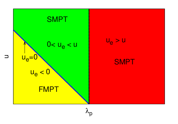
Our analysis of MPTs are only indicative in nature that may be confirmed by detailed numerical studies.

We have thus developed an active hydrodynamic theory for inversion-symmetric mixed membranes. There may be a variety of physical realisations which may be described by our model in the hydrodynamic limit, e.g., a mixed symmetric lipid membrane immersed in an isotropic active fluid or a a mixed symmetric lipid membrane with an active component in a passive fluid. We demonstrate that the interplay between heterogeneity and the active processes in the form of lipid-dependent active tensions leads to nontrivial fluctuation properties of mixed membranes. We establish a direct correspondence between membrane conformation fluctuations and MPTs in mixed lipid membranes, which forms a key result of this work. This can be tested in in-vitro experiments on various physical realizations of our model; membrane fluctuations may be measured by spectroscopic methods [38]. In particular, tagged particle diffusion measurements [7] may be used to validate our results. We welcome construction of lattice-gas type nonequilibrium models which will be particularly suitable to numerically study and verify the results obtained here; see, e.g., Ref. [41]. Our work clearly provides a way to ascertain the sign of $\lambda$ and the nature of MPTs without measuring $\phi$-fluctuations. For a jump in $\sigma_{a}$ or $\kappa_{e}$ at a given $T=T^{*}$, it must be first order MPT; else if $\sigma_{a}$ or $\kappa_{e}(q)$ rises smoothly and diverges at some $T=T_{c}$ as $q\rightarrow 0$, the system displays second order MPT. Furthermore, if $\sigma_{a}|_{disorder}<(>)\sigma_{a}|_{order}$, or equivalently, $\kappa_{e}|_{disorder}<(>)\kappa_{e}|_{order}$, then $\lambda>(<)0$. A mixed lipid membrane immersed in an active isotropic fluid made of actin filaments is a possible in vitro system to study our theory. This may be possible by reconstituted actomyosin arrays on a liposome; see, e.g., Ref. [42] for a related experimental study. ATP depletion methods [43] can be used to control the magnitude of $\lambda$ and $\tilde{\lambda}$. It would be interesting to see how contractile or extensile active fluids [10] affect the couplings $\lambda,\tilde{\lambda}$. The sign of $\lambda_{p}$, crucial in our theory for fixing the order of MPT, may be varied by using different sets of lipids. It may be noted that in the ordered phase separated state with A- and B-rich domains, one may define a $\kappa_{e}$ in a given domain that is A- or B-rich. Measurement of this domain-dependent $\kappa_{e}$ can further yield information about both $\lambda,\tilde{\lambda}$; see Appendix.

So far in the above, we ignored hydrodynamic friction [44]. Even when that is included in our analysis, our general conclusion of a one-to-one correspondence between the membrane conformation fluctuations and the nature of the MPTs holds good. Interestingly with hydrodynamic friction, our results hold true even if the membrane is impermeable, i.e., $v_{perm}=0$; see Appendix. We have neglected the geometric nonlinearities in our analysis above. These originate from the nonlinear forms of the area element and mean curvature in the Monge gauge; see Ref.  [18]. These are irrelevant near the critical point in a scaling sense in the presence of the existing nonlinearities. Across first order MPT these may affect the first order transition temperature $T^{*}$ and order parameter $m$ quantitatively; however, our general conclusions are expected to remain unchanged. We did not include any $\phi^{3}$ or $\phi^{5}$ term in (6) above, as we considered only second order MPT belonging to the Ising universality class in the equilibrium limit. A $\phi^{3}$-term in (6) above would yield an first order MPT in equilibrium; a $\phi^{5}$-term would be irrelevant in a scaling sense in the presence of the $\phi^{4}$-term in (6) above. Beyond its immediate applicability to suitable in-vitro systems, our theory should serve as a basis for studying the physics of phase transitions in live cell membranes. We expect our theory to introduce new directions in the physical understanding of living cell membrane dynamics with new vistas of striking nonequilibrium phenomena. We look forward to experimental tests of our predictions on GPMVs and live cell membrane extracts.

Below we provide a list of symbols and the principal results that form the basis of this work here.

where $\Omega$ is a frequency and $\langle|h(q,\Omega)|^{2}\rangle=\frac{\langle|f_{h}(q,\Omega)|^{2}\rangle}{\Omega^{2}+\Gamma_{h}^{2}\kappa_{e}^{2}q^{8}}=\frac{2D_{h}\Gamma_{h}}{\Omega^{2}+\Gamma_{h}^{2}\kappa_{e}^{2}q^{8}}$. Similarly,

We first assume $\lambda>0$. The membrane becomes generically stiff for all $T$.

Case I : first order MPT at $T=T^{*},\;(\lambda_{p}<0$; see main text). At all $T$

(i) $\Delta_{n}:$ finite. $\Rightarrow$ orientational LRO.

(ii) $\Delta_{h}\sim{\rm ln}~L\Rightarrow$: positional QLRO.

(iii) Effective bending modulus, $\kappa_{e}$ shows a jump across $T^{*}$: $\kappa_{e}(T>T^{*})<\kappa_{e}(T<T^{*})$.

Case II: second order MPT at $T=T_{c}$.

For any $T\neq T_{c}$,

(i) $\Delta_{n}$ is finite and smooth (no jump across $T_{c}$)$\Rightarrow$: orientational LRO.

(ii) $\Delta_{h}\sim{\rm ln}~L$ $\Rightarrow$: positional QLRO.

(iii) At $T=T_{c}$, $\Delta_{n}:$ finite (orientational LRO), in fact further suppressed than its value at $T\neq T_{c}$. On the other hand, $\Delta_{h}\sim{\ln\ln}~L$ at $T=T_{c}$, $\Rightarrow$ positional NLO.

(iv) Effective bending modulus, $\kappa_{e}$ rises smoothly as $T_{c}$ is approached.

Now assume $\lambda<0$: Generic crumpling is introduced at all $T$ giving a finite persistence length.

(i)second order MPT: $\zeta(T<T_{c})<\zeta(T>T_{c})$; $\zeta(T=T_{c})\ll\zeta(T\neq T_{c})$. $\zeta(T=T_{c})$ follows the equation

(ii) first order MPT: $\zeta(T<T^{*})<\zeta(T>T^{*})$.

The authors thank the Alexander von Humboldt Stiftung, Germany for partial financial support through the Research Group Linkage Programme (2016).

References

- [1] B. Alberts, D. Bray, J. Lewis, M. Raff, K. Roberts, J.D. Watson, Molecular Biology of the Cell, 3rd edition (Garland, New York, 1994).
- [2] D. Mizuno et al, Science 315, 370 (2007); B. Stuhrmann et al, Phys. Rev. E 86, 020901(R) (2012).
- [3] M.-J. Huang, H.-Yi Chen, and A. S. Mikhailov, Eur. Phys. J. E 35, 119 (2012); M.-J. Huang, R. Kapral, A. S. Mikhailov, and H.-Yi Chen, J. Chem. Phys. 138, 195101 (2013); see also H. Lodish, A. Berk, C. A. Kaiser, M. Krieger, M. P. Scott, A. Bretscher, H. Ploegh, and P. Matsudaira, Molecular Cell Biology, 6th ed. (W. H. Freeman, 2007).
- [4] S. Ramaswamy, J. Toner and J. Prost, Phys. Rev. Lett. 84, 3494 (2000) discuss a study on protein pumps in a fluid membrane; the membrane in this work, however, is asymmetric under inversion, and hence different from ours.
- [5] For recent reviews, see, e.g., F. A. Heberle and G. W. Feigen- son, Cold Spring Harb Perspect Biol 3, 004630 (2011); K. Simons and J. L. Sampaio, ibid., p. 4697; E. L. Elson et al, Annu. Rev. Biophys. 39, 207 (2010); see also M.E.Cates and J. Tailleur, Annu. Rev. Cond. Mat. Phys., 6, 219 (2015), R. Wittkowski et al, Nat. Comm., 5, 4351 (2014) and J. Stenhammar et al, Phys. Rev. Lett., 111, 145702 (2013) for some recent studies on active MPTs.
- [6] S. L. Veatch et al, Proc. Natl. Acad. Sci. U.S.A. 104, 17650 (2007); S. L Veatch, ACS Chem. Biol. 3, 287 (2008); A. R. Honerkamp-Smith et al, Biophys. J 95, 238 (2008); A. R. Honerkamp-Smith et al, Biochimica et Biophysica Acta 1788, 53 (2009). R. Honerkamp-Smith, B. B. Machta and S. L. Keller, Phys. Rev. Lett. 108, 265702 (2012).
- [7] See, e.g., I. Lee et al, J. Phys. Chem. 119, 4450 (2015) and references therein.
- [8] P. C. Hohenberg and B. I. Halperin. Rev. Mod. Phys. 49, 435 (1977).
- [9] P. M. Chaikin and T. C. Lubensky, Principles of condensed matter physics (Cambridge University Press, Cambridge 2000).
- [10] S. Ramaswamy, Annu. Rev. Condens. Matter Phys. 1, 323 (2010); J.-F. Joanny, J. Prost, in Biological Physics, Poincare Seminar 2009, edited by B. Duplantier, V. Rivasseau (Springer, 2009) pp. 1-32; M. C. Marchetti, J. F. Joanny, S. Ramaswamy, T. B. Liverpool, J. Prost, M. Rao, and R. A. Simha Rev. Mod. Phys. 85, 1143 (2013).
- [11] T. C. Adhyapak, S. Ramaswamy, J. Toner, Phys. Rev. Lett. 110, 118102 (2013); L. Chen and J. Toner, Phys. Rev. Lett. 111, 088701 (2013).
- [12] A. Maitra, P. Srivastava, M. Rao and S. Ramaswamy, Phys. Rev. Lett. 112, 258101 (2014).
- [13] S. Zhou et al, Proc. Nat. Acad. Sc. 111, (2014).
- [14] In-vitro model lipid bilayers are typically inversion-symmetric; see Ref. [6].
- [15] We ignore the bilayer structure; see, e.g., E. J. Wallace et al, Biophys J 88, 4072 (2005); T. Baumgart et al, Annu. Rev. Phys. Chem. 62, 483 (2011).
- [16] L. Peliti and S. Leibler, Phys. Rev. Lett., 54, 1690 (1985).
- [17] T. Banerjee and A. Basu, Phys. Rev. E 91 012119 (2015).
- [18] Statistical Mechanics of Membranes and Surfaces, edited by D. Nelson, T. Piran, and S. Weinberg World Scientific, Singapore (1989).
- [19] A. Safran, Statistical Thermodynamics of Surfaces, Interfaces, and Membranes (Westview Press, 2003).
- [20] G. S. Ayton, J. L. McWhirter, P. McMurtry and G. A. Voth, Biophys J., 88, 3855 (2005).
- [21] Actin filaments are known for lipid-specific interactions, e.g., phosphatidylinositol bisphosphate lipids promote actin polymerization on the membrane; see, e.g., Ref. [1]; see also J. Dinic et al, Biochimica et Biophysica Acta - Biomembranes 1828, 1102 (2013) for studies on lipid raft - actin filaments interactions.
- [22] W. Cai and T. C. Lubensky, Phys. Rev. E 52, 4251 (1995).
- [23] In principle, there can be “active tension” terms in which can originate from active stresses; see, e.g., Ref. [12] above. For a membrane with a fixed background, i.e., with a constant these are just as relevant as the -terms considered in Eq. (8) and are ignored here. See Appendix for additional technical discussions for hydrodynamic damping; see also Ref. [44] below.
- [24] For the full nonequilibrium model, is a temperature-like tunable parameter in the model; may be tuned by controlling the ambient temperature. Obviously, assumes the usual significance of thermodynamic temperature in the equilibrium limit.
- [25] To recover the correct equilibrium limit, one needs to drop the and -terms in (8) and reinsert the and terms in (8). The absence of the and terms in (8) does not affect our analysis of the active membrane fluctuations in the long wavelength limit.
- [26] We do not include active , or -terms. Such terms would survive even for , where as active processes here are assumed to couple with the membrane via mean curvature , and hence all active effects on the membrane should vanish for . This rules out an active term in Eq. (9). In any case, these are no more relevant (in a scaling sense) than those (of equilibrium origin) already exist in (9).
- [27] P.-G. de Gennes, J. Prost, The Physics of Liquid Crystals (Clarendon, Oxford, 1993).
- [28] N. Sarkar and A. Basu, Eur. Phys. J E 36, 86 (2013).
- [29] By this we mean a nonvanishing relaxation rate of in the limit of wavevector .
- [30] In general, should have a -independent constant piece that yields an effective surface tension term in (8); see below. We ignore this for simplicity.
- [31] C. Sykes, J. Prost, and J. F. Joanny, in Actin-based Motility: Cellular, Molecular and Physical Aspects, edited by Marie France Carlier (Springer, New York, 2010).
- [32] N. Gov, Phys. Rev. Lett. 93, 268104 (2004).
- [33] P. Girard et al, Biophys. J. 87, 419 (2004).
- [34] N. Sarkar and A. Basu, Phys. Rev. E 92, 052306 (2015).
- [35] N. Selve and A. Wegner, J. Mol. Biol. 187, 627 (1986).
- [36] S. Katira et al, eLife 5, e13150 (2016).
- [37] T. Banerjee, N. Sarkar and A. Basu, Phys. Rev. E 92, 062133 (2015).
- [38] T. Betz and C. Sykes, Soft Matter 8, 5317 (2012).
- [39] A. T. Dorsey, P. M. Goldbart and J. Toner, Phys. Rev. Lett. 96, 055301 (2006).
- [40] See, e.g., S. Lübeck, J. Stat. Phys. 123, 193 (2006).
- [41] B. B. Machta et al, Biophys. J 100, 1668 (2011).
- [42] M. Murrell, T. Thoresen and M. Gardel, Methods in Enzymology 540, 265 (2014).
- [43] P. Singh et al, Assay. Drug. Dev. Technol. 2, 161 (2004).
- [44] L. Kramer, J. Chem. Phys. 55, 2097 (1971).
- [45] C. DeDominicis, J. Phys. (Paris) 37, Colloque C-247 (1976).
- [46] J. A. Aronovitz, P. Goldbart and G. Muzurkewich, Phys. Rev. Lett. 64, 2799 (1990).
- [47] L. Onsager, Phys. Rev. 65, 117 (1944).