Two-site fluctuations and multipolar inter-site exchange interactions in strongly correlated systems
Abstract
An approach is proposed for evaluating dipolar and multipolar inter-site interactions in strongly-correlated materials. This approach is based on the single-site dynamical mean-field theory (DMFT) in conjunction with the atomic approximation for the local self-energy. Starting from the local-moment paramagnetic state described by DMFT we derive inter-site interactions by considering the response of the DMFT grand potential to small fluctuations of atomic configurations on two neighboring sites. The present method is validated by applying it to one-band and two-band Hubbard models on the simple-cubic 3 lattice. It is also applied to study the spin-orbital order in the parent cubic structure of ternary chromium fluoride KCrF3. We obtain the onset of a G-type antiferro-orbital order at a significantly lower temperature compared to that in real distorted KCrF3. In contrast, its layered A-type antiferromagnetic order and Néel temperature are rather well reproduced. The calculated full Kugel-Khomskii Hamiltonian contains spin-orbital coupling terms inducing a misalignment in the antiferro-orbital order upon the onset of antiferromagnetism.
I Introduction
Magnetic and orbital-ordering phenomena in strongly-correlated materials have been a hot topic in condensed matter research for many years. In particular, transition-metal (TM) oxides and fluorides have attracted a lot of attention due to a complex interplay of their spin and orbital orderings[1]. More recently a lot of research have been focused on the lanthanide and actinide compounds exhibiting ordering of high-ranking multipoles, e.g., CeB6 [2, 3], actinide dioxides AO2 (A=U, Np, Pu)[4], and URu2Si2, where the nature of the ”hidden-order” phase is still hotly debated [5]. Experimental determination of multipole-ordered structures is a complicated task, because the conventional neutron diffraction method is often not applicable in this case [4].
Dipolar and multipolar moments in those materials are carried by localized shells of correlated and electrons. First-principles description of such strongly correlated compounds is nowadays possible using a combination[6, 7] of density-functional-theory (DFT) band structure techniques with the dynamical mean-field theory (DMFT) treatment[8] of correlated electrons. This approach is particularly efficient in capturing the high-temperature symmetry-unbroken state. There are no principal limitations for applications of the same method to symmetry-broken ordered phases. However, typical low ordered temperatures and low symmetries of those phases as well as a vast configuration space of possible ordered states render direct predictive DFT+DMFT calculations in this case rather difficult. Moreover, the single-site DMFT method suffers from the usual mean-field drawbacks overestimating ordering temperatures, especially, for low-dimensional systems (see, for example, Ref. 9, 10, 11, 12, 13, 14).
Hence, a promising approach for a first-principles description of orbital and multipolar ordering phenomena consists in using the DFT+DMFT method to evaluate an effective low-energy Hamiltonian describing inter-site interactions between localized shells. Such Hamiltonians can then be solved by a variety of methods developed for Heisenberg and similar models in order to predict the ordered phase as a function of external parameters like pressure or temperature.
Several such techniques have been proposed [15, 16, 17, 18, 19, 20, 21] for evaluating low-energy spin Hamiltonians in conjunction with standard DFT methods. They were subsequently also extended to calculations, for example, of the magnetic crystalline anisotropy [22] and Dzyaloshinskii-Moriya interactions[23] . Generally, in those approaches effective exchange interactions are extracted by considering a first-order response of the grand potential upon a simultaneous change of magnetic configurations of two neighbouring sites. In particular in those approaches that have been to date generalized for correlated systems (Refs. 24, 25, 26), one computes the variation of the grand potential of a magnetically-ordered state upon simultaneous small tilting of two neighbouring spins.
The technique proposed in this work in order to calculate inter-site dipolar and multipolar interactions is similar in spirit to those methods. However, in contrast to them, we will calculate the variation of the DFT+DMFT grand potential of a paramagnetic (symmetry-unbroken) phase upon simultaneous small change of the atomic configurations of correlated shells of two neighboring sites. Hence, one can derive inter-site interactions directly from the high-temperature paramagnetic state, which is typically most readily accessible for DFT+DMFT. The approach is currently formulated using the atomic (Hubbard-I)[27] approximation for the DMFT local self-energy. It is fast and, in principle, able to calculate all terms of the low-energy Hamiltonian, including non-Ising spin-spin, spin-orbital and multipolar interactions. The formulation on the basis of Hubbard-I entails, however, certain limitations. In particular, the present approach is suitable for localized systems like TM oxides and local-moment lanthanide compounds and cannot be applied to metals.
As first application of this technique to real materials we study the spin-orbital ordering in the cubic phase of the Mott insulator KCrF3. In this compound the 3 shell of the Cr2+ ion is in the high-spin configuration with the spin of single electron aligned to that of the half-filled subshell by the Hund’s rule coupling, similarly to undoped peroxide manganese LaMnO3. KCrF3 adopts the cubic peroxide structure at high temperatures. At K it undergoes a first-order orbital-ordering transition accompanied by a tetragonal distortion (space group )[28]. Another structural transition to a low-temperature monoclinic phase (space group ) due to tilting of the CrF6 octahedra is observed at K[29]. Finally, a transition into an incommensurate layered antiferromangetic (AFM) phase with the ordering vector (1/2, 1/2, 0) in the monoclinic cell is taken place at K[30]. Below 46 K the AFM order becomes a fully commensurate A-type one with , a spin canting is detected below 9.5 K leading to formation of a small ferromagnetic moment [30].
As in other Jahn-Teller systems it is important to disentangle the lattice and purely electronic superexchange contributions into the spin-orbital ordering in KCrF3 to understand their relative importance. Previously the orbital ordering in the undistorted cubic structure has been studied theoretically within DFT+DMFT[31] and DFT+U[32, 33] approaches. In particular, the authors of Ref. 31 derived an effective DMFT impurity problem for the Cr subshell with a simplified treatment of its interactions with the spin, which was subsequently solved by a quantum Monte Carlo (QMC) method. They obtained a substantially underestimated value K when only the supexchange contribution was taken into account.
Here we compute all relevant superexchange interactions for the cubic phase of KCrF3 and then solve the resulting effective spin-orbital Hamiltonian within mean-field obtaining orbital and magnetic ordering temperatures and the corresponding phases. We find an underestimated value of in agreement with Ref. 31, in contrast, the calculated value for and the predicted A type of the AFM order agree with those experimentally observed in KCrF3. We show that the onset of the AFM phase produces a feedback effect on the orbital arrangement leading a loss of the perfect antiferro-orbital order even in the absence of lattice distortions.
The rest of paper is organized as follows: the method is derived in Sec. II. It is subsequently tested and its limitations explored by applying it to one-band and two-band Hubbard model on the simple-cubic lattice in Secs. III and IV, respectively. Finally, its application to KCrF3 and the obtained results are presented in Sec. V.
II Method
We start by deriving in Sec. II.1 variation of the Hubbard-I self-energy with respect a change of the atomic configuration of correlated shell . The derived expressions are then used in Sec. II.2 to calculate the variation of the DFT+DMFT grand potential upon simultaneous change of atomic configurations on two neighboring sites and, thus, to extract the corresponding inter-site interactions between those configurations. Finally, in Sec. II.3 we recast the obtained interactions into a more conventional dipolar and multipolar form. The full calculational procedure is shortly outlined in Sec. II.4.
II.1 Local fluctuations within the Hubbard-I approximation
Let us first outline the main features of the Hubbard-I approximation (HIA) as applied to the DMFT quantum impurity problem. In this case the HIA can be derived by a high-frequency expansion of the DMFT self-consistency condition (see, e.g., Ref. 34) to the first order in , leading to the following expression for the non-interacting level positions of the impurity:
| (1) |
where and are the Kohn-Sham(KS) Hamiltonian and ”projector” between the KS and correlated spaces for a given point in the Brillouin zone (BZ), respectively, is the double-counting correction for the self-energy, is the chemical potential, is the unit matrix. The DMFT bath Green’s function within the HIA takes a very simple form
| (2) |
where is the fermionic Matsubara frequency. Solving of the impurity problem is then reduced to the diagonalization of the effective atomic Hamiltonian , where () is the creation(annihilation) operator for the localized orbital labeled by relevant quantum numbers designated by (), is the on-site Coulomb repulsion.
The corresponding atomic Green’s function then reads
| (3) |
where and are eigenstates of the atomic Hamiltonian , and are the corresponding eigenenergies and Boltzmann weights, respectively, is the partition function, is the inverse temperature. The atomic self-energy can then be calculated through the Dyson equation:
| (4) |
In cases where the HIA is applicable and for reasonable temperatures the system is far from the intermediate-valence regime, hence, charge fluctuations can be safely neglected. Moreover, in localized systems the most important fluctuations are expected to occur among quasi-degenerate states belonging to the ground-state (GS) atomic multiplet. For example, for 4 shells this multiplet is defined by the occupancy as well as by the spin , orbital and total quantum numbers, in TM ions it is rather defined by the occupancy, , and crystal field. In solids the GS multiplet can be additionally split by smaller energy scales, like the crystal field in rare-earths and the spin-orbit coupling in TM ions. Hence, here we consider fluctuations only among the states belonging to GS multiplet. It is useful for the following to recast the atomic GF into a slightly more general form:
| (5) |
where the first term comprises all contributions to involving the states of the GS multiplet; those states will be in the following designated by capital Greek letters, for example, . The rest is collected in . The density matrix (throughout Sec. II we use the hat, , for any matrix in the basis of atomic states ) of the GS multiplet in the symmetry-unbroken (paramagnetic) state is defined within the HIA by
| (6) |
where is the Kronecker delta, and the corresponding element of the atomic GF matrix in the imaginary time domain reads , where is the time-ordering operator, and are eigenstates of belonging to the GS multiplet. By the Fourier transform one obtains, e.g., for the off-diagonal matrix elements of in the frequency space:
| (7) |
where , is the energy difference between the state belonging to the GS multiplet with the occupancy and the excited state . Similar, but simpler expressions can be obtained for the diagonal elements .
Let us now consider the change of the atomic Green’s function upon a small fluctuation of the density matrix with respect to its symmetry-unbroken Hubbard-I form (6). We define the fluctuation for diagonal elements as a diagonal matrix with the following elements:
| (8) |
where is the degeneracy of the ground-state multiplet, is a small parameter. As one may easily see, the fluctuation (8) conserves the trace of and induces a corresponding fluctuation of an angular moment of the shell. For example, if in the symmetry-unbroken state the value of an angular moment operator is zero, and , then the corresponding fluctuation of the moment is .
We also define the off-diagonal fluctuation of as an matrix with a single none-zero element:
| (9) |
Using the definition (5) for the atomic GF one then obtains the following expression for the variational derivative of over a fluctuation of the type (8) or (9):
| (10) |
The second term in (5), , does not contribute to the variational derivative (10), because the weights of the states not belonging to the GS multiplet are not affected by fluctuations of the types (8) and (9). Those fluctuations only redistribute the weights within the GS multiplet and do not change .
The corresponding variational derivative of the atomic self-energy (4) reads:
| (11) |
II.2 Response of the grand potential and effective inter-site interactions
| (12) | |||
where is the electronic density, is the Kohn-Sham one-electron potential, is the local GF, is the difference between the impurity self-energy and the double counting correction , is the DMFT interaction energy functional for the site , is the corresponding functional for the double-counting correction, is the chemical potential. The last term depends only on the electronic charge density , while all other terms collected in do not have an explicit dependence on . At the DMFT self-consistency the local GF of the lattice problem should be equal to the impurity GF . Within the HIA, however, the full DMFT self-consistency is never achieved because the hybridization function is neglected in the impurity problem, , but is included into the local GF of the lattice problem. Hence, within the HIA one should always keep the distinction between and , where and calculated within the HIA in accordance with (3) and (4), respectively.
Let us now introduce the basis of Kohn-Sham eigenstates , where labels Kohn-Sham bands. The corresponding real-space (Wannier) basis functions are defined by , where is the unit cell volume 11 1 The Wannier transformation is gauge-invariant with respect to a unitary transformation of . For the present derivation it is not important, hence, we assume that the corresponding unitary matrix is equal to unity.. We also introduce a real-space basis of (localized) Wannier orbitals representing correlated states, , where labels orbitals at the correlated shell , as well as corresponding projectors between the KS and correlated subspaces, . Using the real-space bases and and within the HIA one may rewrite as follows:
| (13) |
where elements of the real-space matrix read
| (14) | ||||
and are matrices in the band and correlated orbitals’ spaces, respectively, the matrix elements of the former are given by .
We will now calculated the response of the grand potential (12) upon simultaneous fluctuations of atomic configurations of correlated shells on two different atomic sites, i.e. we evaluate . First, in the usual ”force theorem” spirit [37, 19, 38] one may neglect, to the first order in , the contribution due to the renormalization of the charge density, i.e., the contribution from . One may also notice that all terms in (13), apart from the first one, are site-diagonal and will not contribute to a variational derivative over configurations of two different sites. Hence, the only non-zero contribution due to simultaneous fluctuations on two different sites and is due to the first term in (13). dependence on the correlated shell configuration stems from that of the atomic self-energy . The double-counting correction for a paramagnetic phase depends only on the total shell occupancy, which is not affected by the density-matrix variations (8) and (9). Performing the derivative and making use of the ”folding” property of projector matrices, one obtains
| (15) |
where the derivative over an on-site fluctuation is given by eq. (11), etc. is the relevant set of quantum numbers labeling the state and the ”inter-site” GF can be calculated as a Fourier transform of the DMFT lattice GF in the reciprocal space:
| (16) |
In eq. (15) we identify with the corresponding inter-site interaction of an effective low-energy Hamiltonian of the system:
| (17) |
where is the corresponding projection (Hubbard) operator between the atomic states and belonging to the ground-state multiplet of the site , is the one-site (crystal-field) term, is the inter-site interaction between the corresponding Hubbard operators on the sites and (here the label is suppressed and the short-hand notation is used).
The identification of the corresponding inter-site interaction in with (15) can be justified using, e.g., the approach of Refs. 39, 40, 36. Using this approach one may write a (Legendre-transformed) grand potential corresponding to (17) for a set of preassigned on-site occupancy matrices as , where and is the mean-field and beyond-mean-field contributions, respectively, is the one-site term. Setting the density matrices to their mean-field values in the symmetry-unbroken state and computing the variational derivative of over one obtains . Hence, one identifies the derivative (15) of the dynamical mean-field grand potential (12) as the corresponding inter-site interaction in (17). Of course, the usefulness of those interactions depends on whether the effective Hamiltonian (17) indeed describes the low-energy physics of (12). This should be the case for strongly-correlated local-moment systems, e. g., for rare-earth intermetallics above their Kondo temperature or for Mott insulators.
II.3 Multipolar formalism
The inter-site interactions between atomic states calculated in accordance with (15) can be used directly, e.g., in an effective Hamiltonian of the type (17). This Hamiltonian is written in terms of low-energy interactions between the on-site Hubbard operators defined above describing transitions between atomic states belonging to the ground-state multiplet.
However, the standard dipolar and multipolar tensor operators are, in fact, linear combinations of those Hubbard operators with coefficients written in terms of of the corresponding Wigner 3 symbols[4, 41]. Hence, instead of working directly with the Hubbard-operator form (17) one may recast this Hamiltonian to describe interactions between dipole and multipole (quadrupole, octopole, etc.) operators acting on neighboring sites. The low-energy Hamiltonian in this form is more standard (one may recall, for example, the spin Heisenberg and spin-orbit Kugel-Khomskii Hamiltonians) and also more compact when additional symmetries are present. Moreover, it is written in terms of operators which expectation values , i. e. dipole and multipole moments, are directly measured experimentally. In this section we derive a transformation relating inter-site interactions in the density-matrix (17) and more conventional dipolar-multipolar Hamiltonians.
We start by briefly summarizing properties of tensor operators. The spherical tensor operators in the basis of angular-momentum eigenstates are standardly defined as follows [4, 41]:
| (18) | ||||
where and label the multipole rank and component, respectively, states belong to the ground-state multiplet specified by the angular-momentum quantum number , , is the Hubbard operator acting within the ground-state multiplet, the coefficients read:
| (19) |
The set of operators with , (i.e., monopole, dipole etc. operators) and is complete in the subspace spanned by the states and any operator acting in this subspace can be represented as a linear superposition of . Other properties of those operators are discussed, e.g., in Refs. 4, 41. In particular, one may notice that the tensor operators (18) cannot represent observables as they are not self-adjoint[41], , for . However, the self-adjoint linear combinations of can be formed similarly to the real spherical harmonics:
| (20) |
where
| (21) | |||
for and , respectively. For example, for the dipole, , the components equal to , , and transform under rotations as Cartesian , , and , respectively, similarly to the corresponding real spherical harmonics.
One may introduce inter-site interaction between the tensor operators (20) acting at sites and as , where the tensor operators of the rank () and for the component () are defined for the ground-state multiplet of the corresponding atomic shell (), respectively. The label in is suppressed here to simplify the notation. It is easy to show that is equal to the inter-site interaction defined in (15) and (17).
By making use of the orthogonality relations of the 3-symbols one may also show that . Then by multiplying the inter-site interactions (15) by and and summing over the quantum numbers one obtains
| (22) |
Using (22) one may transform the inter-site interactions from the atomic-level, eq. (15), to mutipolar form 22 2 One may notice that off-diagonal interactions with and/or may carry an arbitrary complex phase, which will then be passed to . To avoid this we require that states used in (7) and (18) satisfy the usual phase convention with the matrix element of the ladder operator being a real positive number..
In many cases inter-site interactions and corresponding ordering temperatures come out to be much smaller than the crystal field (CF) splitting within the ground-state multiplet . In this case one may restrict oneself to determining inter-site interactions between the states belonging to the lowest CF level. For example, one may represent the state of an TM ion by a product of the ordinary spin and pseudo-spin quantum numbers, with the opposite directions of the pseudo-spin corresponding to the and orbitals, respectively. This representation is widely used for TM oxides [1]. In this case one may introduce another type of tensor operators, the double tensor, which is a direct product of two spherical tensors for and can be written using (21) as follows:
| (23) | ||||
where we again use the corresponding Hubbard operator . The subscripts and superscripts in are the ranks and components, respectively, of the single tensors forming the direct product. Then, for example, in the ”double” spin-orbital space and will designate the spin and orbital dipole tensors, respectively, with , , or . Analogously, spin-orbital combined tensors can be also introduced for the case of KCrF3 or other compounds with the high-spin shell, the only difference is that the tensor is used in this case to describe the spin.
Similarly to (22) the corresponding interactions read
| (24) |
where the short-hand notation is used. Finally, instead of using the tensors as defined in eqs. (20) and (23) one may wish to write the interactions in terms of more conventional spin operators for the dipole case and the unit matrix for the monopole one, respectively, by renormalizing the inter-site interactions as follows:
| (25) |
where the factor is equal to and for equal to 0 and 1, respectively [41].
We will label those interaction by and for the dipole orbital and spin moments, respectively, as well as by for the dipole-dipole (”quadrupole”) spin-orbital one. For example, is the spin-spin dipole-dipole interaction, is the orbital-orbital dipole-dipole one, is the orbital-(spin-orbital) dipole-quadrupole one and so on. Finally, for the case of one atom per unit cell we may always make use of the translational invariance, hence, can be substituted with .
II.4 Outline of calculation procedure
Let us summarize the sequence of steps for calculating inter-site interactions using the method described above.
First, one carries out full self-consistent DFT+DMFT calculations using the Hubbard-I approximation as the impurity solver. Second, one computes the atomic Green’s function matrix elements (7) and the variation derivative of the atomic self-energy (11) as well as the inter-site DMFT Green’s function in the real-space (16). Finally, the inter-site interactions are computed in accordance with (15) and then transfomed, if desired, into a suitable multipolar form using (22) or (24). The method is implemented numerically using the TRIQS library[42].
III One-band Hubbard model
In this section we benchmark the approach presented in Sec. II by applying it to a simple example of the one-band particle-hole symmetric Hubbard model on the 3 simple cubic lattice. The Hamiltonian of this model reads

| (26) |
where belongs to the first Brillouin zone of the simple cubic lattice, is the number operator for the site and spin . For the simple cubic lattice with the nearest-neigbour hopping the band energy , where are in units of the inverse lattice spacing . Applying the Hubbard-I approximation in the framework of DMFT to as described in Sec. II.1 and under the condition of one obtains and for the atomic GF (3) and self-energy (4), respectively. Then one may easily obtain inter-site interactions of the effective low-energy model at analytically by computing the inter-site GF using the Fourier transform (16) and the variational derivatives of the atomic self-energy using eqs. (7) and (11), respectively, and then inserting the result in (15). For example, by inserting the nearest-neigbour inter-site GF and the ”off-diagonal” derivative of the atomic self-energy ( is the same expression transposed)
into (15) and carrying out the summation over Matsubara frequencies and spins one obtains for the nearest-neighbor spin-off-diagonal matrix element (where the lattice vector connects nearest neighbors). This is indeed the correct value for this matrix element of the low-energy model for at , which is well known to be the spin-1/2 Heisenberg model
| (29) |
where the interaction is isotropic and depends only on the distance , i.e. on the coordination shell . In the lowest order in only the nearest neighbor anti-ferromagnetic interaction survives in .
We have calculated numerically all matrix elements of (29) for several first coordination shells as a function of U/t using (15) and then applied the transformation (22) to obtain the corresponding inter-site interactions between the dipole tensor operators for spin 1/2. As expected, those interactions come out to be isotropic and direction-independent, . Finally, the tensor interactions are renormalized, (cf. eq. 25), for the standard angular-momentum-operator form (29) of the Heisenberg Hamiltonian . Resulting are plotted in Fig. 1 as a function of . One sees that deviates stronger from the asymptote with increasing and, simultaneously, the second and third coordination sphere interactions increase though they still remain quite insignificant compared to .

The calculated interactions have been used to evaluate the value of Néel temperature for the model (26) within the mean-field approximation. The obtained values are compared in Fig. 2 to calculated within single-site DMFT using numerically-exact quantum Monte-Carlo (QMC) techniques [44, 43, 10]. The agreement with these numerically-exact is good for . We note that within the dynamical mean-field theory Heisenberg not only define the transition temperature but also directly impact spectral properties of the Néel phase. In fact determine the spin-polaron peak structure within the Hubbard bands[45, 46], which can be in some cases detected in real Mott insulators[46]. Hence, one may suggest that the present approach can be possibly used to provide parameters for -like models aimed at investigating those phenomena.
For the present approach deviates significantly from the exact mean-field values, though less strongly than the simplest large- asymptote. The value of at which the maximum of exact mean-field is reached is very close to the critical value of for the metal-insulator transition in the paramagnetic phase [47]. Hence, one concludes that the present approach is reliable in the Mott-insulating regime.
IV -orbital Hubbard model
Here we apply the method of Sec. II to a more complex model system, a two-band Hubbard model on the 3 simple cubic lattice, given by
| (30) |
where runs over nearest-neighbor bonds, and label orbitals, is the corresponding element of the hopping matrix, is the on-site interaction term. We assume the orbitals to belong to the representation of the cubic group for , and , and employ the corresponding relations between the nearest-neighbor hopping integrals , in which case the Fourier-transformed hopping matrix reads:
| (31) |
where is the hopping between two orbitals for along the axis. By diagonalizing (31) one obtains band dispersions with the total bandwidth .
| (32) | ||||
where and are the Coulomb and Hund’s rule interactions, respectively.
We study the case of one-quarter filling, , for which the model (30) is relevant for a number of transition-metal compounds, for example, potassium copper fluorite KCuF3 [1, 50, 48] and rare-earth nickelates NiO3[51, 52, 53]. Essentially the same model was studied within DMFT in various parameter regimes to understand the behavior of nickelate-based heterostructures[54, 55, 56]. The magnitude of super-exchange antiferromagnetic coupling is believed to be a crucial parameter controlling the physics of those heterostructures [54, 57].
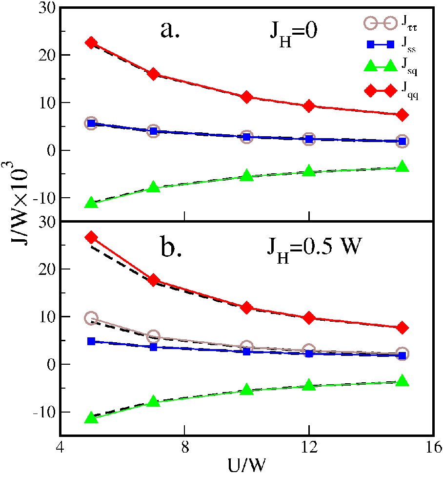
We first carried out DMFT calculations employing the HIA with set either to 0 or to 0.5 and being in the range from 5 to 15. The lower limit of is chosen to be above the critical value (where the prefactor lies in the range from 1.5 to 2.5 depending on the lattice type under consideration) for the Mott transition in the two-band Hubbard model at quarter filing [58, 59, 53]. Then the superexchange inter-site interactions at the first coordination shell between four one-electron states , , , and were computed in accordance with (15). Finally, we employed eqs. (24) and (25) to recast them into the standard Kugel-Khomskii[1] form of interacting spin-1/2 operators and representing spin and orbital degrees of freedom, respectively ( and designate occupied and , respectively). The resulting effective Hamiltonian for the [001] bond, , reads
| (33) |
where , , , and are the spin-spin, orbital-orbital, spin-(spin-orbital) and (spin-orbital)-(spin-orbital) interactions defined in Sec. II.3, respectively, runs over , , and . As expected, the calculated effective Hamiltonians for the [100] and [010] bonds are related by the cubic symmetry to and can be obtained from it by the corresponding rotation in the space, i. e., by substituting in (33) with and , respectively.
The calculated values of , , , and vs. are displayed in Fig. 3 together with the corresponding values of those superexchange interactions obtained from the analytical expressions derived in Refs. [50, 48]:
| (34) |
where , with being the average Coulomb repulsion between electrons with opposite spins. One may note a perfect agreement between the calculated and analytical values in Fig. 3a for the case , for which eqs. (34) reduce to . In the case of (Fig. 3b) there are small discrepancies between the present approach and the analytical formulas (34) at low values of . This is apparently due to the fact that the formulas (34) were derived[48] by the first-order expansion in and become less accurate with increasing .
V Spin and orbital ordering in KCrF3
In this section we calculate ab initio superexchange interactions for the cubic phase of KCrF3 and then employ the resulting effective Hamiltonian to compute ordered phases and transition temperatures within the mean-field approximation.
First we carried out DFT+DMFT calculations of KCrF3 using the linearized augmented plain-wave (LAPW) band structure method as implemented in the Wien2k[60] code in conjunction with the DMFT and HIA implementations provided by the TRIQS library[42, 61]. The Wannier orbitals representing correlated Cr 3 states were constructed using the projective approach of Ref. 62 from the Kohn-Sham (KS) states in the window [-2.7:2.7] eV around the Fermi level, this window encloses both and -like KS bands. The self-consistency over the charge density in the DFT+DMFT calculations was implemented as described in Ref. 63, the spin-orbit coupling was neglected.

The rotationally-invariant local Coulomb repulsion between all five Cr 3 orbitals was parametrized by the Slater integrals eV, as well as eV and eV corresponding to the Hund’s rule coupling eV. Those values of and eV were computed for KCrF3 in Ref. 31 using a constrained-LDA technique. We also performed calculations with eV for the sake of comparison. We employed the fully-localized-limit form for the double counting correction term calculated with the nominal Cr 3 shell occupancy of 4, this choice was shown to be appropriate for the HIA [34].
KCrF3 was calculated in its high-temperature cubic peroxide structure with the experimental[28] lattice parameter of 4.23 Å. We employed the atomic sphere radii of 2.5, 2.0 and 1.78 a.u. for K, Cr and F, respectively. The Brillouin zone (BZ) integration was carried out using 4000 k-points in the full BZ, test calculations showed that increasing further the density of the k-mesh had a negligible effect on the values of superexchange interactions.
Our DFT+DMFT calculations within HIA predict KCrF3 to be a Mott insulator. Its spectral function features a Mott-Hubbard gap of about 2 eV, with the gap edges formed by -like bands, see Fig. 4. The high-spin configuration with the total spin is predicted to be the ground-state multiplet of the Cr 3 shell, as expected. Due to the orbital degeneracy of and the total degeneracy of the ground-state multiplet is .
Effective inter-site interactions (15) between those 10 states belonging to the ground-state multiplet were then calculated in accordance with the approach of Secs. II.1 and II.2. Then we again made use of eqs. (24) and (25) to recast them into the Kugel-Khomskii form.
The calculated interactions between second nearest neighbors and beyond are at least two orders of magnitude smaller then those between the nearest neighbors and were neglected. The calculated superexchange Hamiltonian between two nearest neighbors and along the [001] direction has the following form
| (35) | |||||
where and run over , , and , , respectively. The spin operators act in the space of the total spin of the site , the and quantum numbers designate the and shell configurations, respectively. The meaning of , , and is the same as in eq. (33) of Sec. IV. Comparing (35) to (33) one notices the appearance of new and terms. Because there is no inter-orbital hopping within the subshell along the axis those terms should be related to virtual hopping of electrons (hence, they are absent from the pure model, eq. 33 )33 3 While there is no symmetry reason for the interactions of and to be equal we found them to be almost coinciding..
| U (eV) | ||||||
|---|---|---|---|---|---|---|
| 3.75 | 0.94 | 37.3 | 1.71 | -1.77 | 7.12 | 0.28 |
| 5 | 0.96 | 24.7 | 1.20 | -1.43 | 4.93 | 0.21 |
In Table 1 we list the values of the inter-site interactions calculated with eV and eV. One sees that the orbital-orbital and (spin-orbital)-(spin-orbital) interactions are the most significant ones, even if one takes into account the different lengths of and spins. These interactions exhibit a strong reduction upon increasing and decreasing , cf. (34). The (spin-orbital)-(spin) term is also significant. and are more than one order of magnitude smaller than and , respectively.
We have then solved the calculated nearest-neighbor superexchange Hamiltonian defined by eq. 35 (the nearest-neighbor interactions along the [100] and [010] directions are obtained from (35) using rotations in the space as described in Sec. IV) within the mean-field approximation using McPhase package [64] obtaining the total and free energies as well as stable ordered phases as a function of temperature.
The calculated temperature dependence of the specific heat (see Fig. 5a) features two clear phase transitions at temperatures of 340 and 102 K. The high-temperature one is an orbital-ordering transition, the obtained antiferro-orbital structure is displayed in Fig. 5b. The occupied states on two inequivalent sites, (which are the nearest neighbors in the simple-cubic Cr sublattice, see Fig. 5b) in this structure can be written as
| (36) | |||
| (37) |
with , hence, the obtained structure corresponds to a G-type antiferro-orbital order with the empty orbital on the site one being occupied on the site two 44 4 The notation used in eqs. (36) and (37) follows that used in Ref. 28. Another representation of the G-type antiferro-orbital order is more standard in the case of LaMnO3 (see, for examle, Ref. 68) and obtained by substituting in (36) and in (37) with and , respectively. The actual value of the angle is not defined by the Hamiltonian (35) in the absence of the spin ordering, experimentally it is fixed by the tetragonal lattice distortion and equal to 30∘[28]. In fact, neglecting the lattice distortion leads to a strongly underestimated value of the temperature for the orbital ordering compared to experimental 973. The same result was obtained by Autieri et al. [31] using direct DMFT+QMC calculations and was shown to be due to the on-site crystal field splitting, the renormalization of hopping integrals due to the tetragonal (and subsequent monoclinic) distortion had an insignificant effect on .

The low-temperature transition at K is due to ordering of Cr spins into the AFM A-type structure shown in Fig. 5c. This structure consists of an antiferromagnetic stacking of ferromagnetically-ordered layers, with each Cr site having four in-plain neighbours with the same spin and two out-of-plain ones with the opposite spin. This, in fact, is the collinear spin structure observed experimentally in KCrF3. The obtained Néel temperature is in good agreement with experimental value of 80 K[30], if one takes into account the usual mean-field overestimation of ordering temperatures. Hence, one sees that once the orbital order sets in the superexchange is able to account for the value of and observed collinear magnetic structure even without including lattice distortions 55 5 A possibility for slight non-collinearity as the one present in KCrF3 between 46 and 80 K was not considered in the mean-field solution of the effective Hamiltonian. Also our simulations neglect the spin-orbit couping and, hence, are not able to reproduce the spin canting observed below 9 K.
We have also performed the same mean-field calculations with the effective interactions computed with eV, obtaining the same orbitally-ordered structure at somewhat lower temperature of 225 K. The obtained low-temperature spin structure is, however, different, it is of the C-type and consists of an anitferromagnetic stacking of ferromagnetically-ordered [101] plains. Hence, each site has two nearest-neighbors with the same spin and four with the opposite one, see Fig. 5d.
In order to clarify the origin of this change of magnetic order with increasing one may carry out a simple estimate of the energy of the A-type and C-type AFM spin structures. First, keeping in (35) only the most important and contributions and summing over all nearest-neighbors one obtains for the mean-field spin-ordering energy (per formula unit, f.u.) of the A-type structure
| (38) |
where is the overall spin factor, which for the case of high-spin Cr2+ can be rather well approximated by the square of its classical length, at the full saturation, and label two sublattices of the G-type antiferro-orbital structure. The energy of the C-type structure is given by the same expression with the minus sign.
The energies of the ferromagnetic (FM) and G-type AFM (all nearest neighbors having the opposite spin) phases are
| (39) |
where the plus/minus sign is for the FM/AFM case, respectively. One may notice that is always equal to -1/4 for the fully saturated G-type antiferro-orbital order and does not dependent on the angle in eqs. (36) and (37). Hence, the total energy of the FM and G-type AFM order is also independent of .
Assuming a fully-saturated G-type antiferro-orbital order, i. e. , and , and minimizing (38) one obtains with the orbital state fixed at and , defined by in (36). For the C-type structure one has and the orbital state locked at and , corresponding to (which is, in fact, the experimental orbital state in tetragonal KCrF3). The energies of the FM and G-type AFM orders do not dependent on as explained above and are equal to , respectively. Hence, one sees that the spin order is defined by the ratio of , which increases with decreasing (increasing ), see Table 1. For eV and eV one obtains for the energy difference the values of 2.75 and 0.4 meV per f.u., respectively. Hence, at the realistic value of eV those two structures are almost degenerate, though is still the most stable. The G-type AFM and FM structures are always higher in energy, in particular, for eV their energies are 6.7 and 7.9 meV per f.u. above .

Further analysis shows that the A-type structure is stabilized at eV due to the term, which upon the onset of antiferromagnitism acts as a canting field in the orbital space. For the C-type structure it takes the form and one may show that under the corresponding G-type antiferro-orbital order given by it is not active as long as . The system stays in the same antiferro-orbital state with , for which the contribution of the term to the energy is zero. For the A-type structure it takes the same form with the minus sign, but now under the different orbital state given by and () it does play a role leading to a loss of the perfect G-type antiferro-orbital order. Namely, upon the onset of the A-type spin order the angles and defining the corresponding orbital states (36) and (37) on two sublattices start deviating from each other, the corresponding loss in the orbital ordering energy is compensated by the ”orbital field” due to . The corresponding difference (extracted from mean-field solution of the full effective Hamiltonian, eq. 35) grows with decreasing temperature due to increasing spin moment, as shown in Fig. 6. This orbital misalignment stops increasing once the magnetic moment fully saturates below approximately 30 K. The total gain in energy due to this misalignment of about -1.4 meV/(f.u.) is rather small compared to the total energy of the spin-orbital ordering of -22.9 meV/(f.u.), but it is sufficient to stabilize the A-type antiferromagnetic order.
Previously the interplay of orbital ordering and the A-type AFM structure has been intensively studied in the case of the Mn peroxide LaMnO3, where Jahn-Teller lattice distortions were proposed to be at the origin of this AFM structure, see, for example, Refs. 23, 67, 68. The dependence of the relative stability of different magnetic phases of LaMnO3 on was previously demonstrated in a model study of Ref. [69]. KCrF3 features some similarities to this system, though in LaMnO3 the orbital order is of the C-type instead of the G-type. Direct ab initio DFT+U calculations[32, 33] for cubic KCrF3 predicted a ferro-orbital order to be stabilized in conjunction with the A-type AFM, in disagreement with our results and experiment. Apparently, this is due to an incorrect relative scale of spin- and orbital-ordering energies in DFT+U within the local spin-density approximation, where the orbital order is seen to be induced by the underline AFM state[32]. As one sees from Table 1, the inter-orbital superexchange is the strongest interaction, hence the AFM state emerges well below from an almost completely saturated G-type antiferro-orbital order, in agreement with experiment. In our description the angle , which defines the orbital state (36) , is fixed by the lowest-energy AFM order, in real KCrF3 it is rather fixed by the distorted lattice. The tetragonal distortion favors the C-type AFM in accordance with our calculations, however, experimentally the magnetic order emerges in the lower-temperature monoclinic structure, in which the orbital state is possibly more favorable to the A-type magnetic order. It is interesting to observe that even in the absence of any lattice distortions the feedback effect described above leads to a canted orbital order in conjunction with the A-type AFM. Experimentally one may also expect to observe an additional small titling/distortion of the CrF6 octahedra upon the onset of antiferromagnitism, though our calculations predict a rather small energy scale associated with this process, of the order of 1 meV.
VI Summary
We have presented a method for computing inter-site exchange interactions in correlated materials in the framework of the DFT+DMFT in conjunction with the Hubbard-I approximation to the DMFT self-energy. The expressions for inter-site interactions are derived by considering the first-order change in the DFT+DMFT grand potential to simultaneous small fluctuations on two atomic sites with respect to their symmetry-unbroken paramagnetic configuration. The resulting expression (15) combines the variational derivatives of the Hubbard-I self-energy (11) over a given fluctuation in the on-site density matrix with the DMFT inter-site Green’s functions (16). The method is benchmarked by applying it to the well-known cases of one-band and two-band Hubbard models on the simple-cubic 3 lattice.
The presented technique has been already employed to compute spin-spin superexchange interactions in cubic and quasi-two-dimensional tetragonal TM oxides [14]. Here we have applied it to a more complex case of spin-orbital ordering in KCrF3 in its parent undistorted peroxide structure. We obtained an effective Hamiltonian (35) featuring strong antiferro-orbital nearest-neighbor interactions and a complex anisotropic coupling between orbital and spin moments. By solving it within the mean-field approximation we found the onset of a G-type orbital order at a significantly lower temperature as compared to experiment. In contrast, the appearence of experimentally-observed A-type antiferromagnetic structure is predicted at K in good agreement with experiment. The onset of A-type antiferromagnetism is explained by purely superexchange mechanism as arising due to an interplay of the spin-spin and (spin-orbit)-(spin-orbit) inter-site couplings in conjunction with a canting of the G-type antiferro-orbital order. Further applications of this technique to the tetragonal and monoclinic structures of KCrF3 should help to clarify whether this mechanism for the stabilization of the A-type magnetic structure is qualitatively affected by the lattice distortions.
The present method is promising for applications to a wide range of strongly-correlated materials, like spin-orbital order in TM oxides and florides as well as multipolar ordering due to localized shells in rare-earth and actinide materials. It would be interesting to consider its generalizations beyond the Hubbard-I approximation to widen its range of applicability to materials located close to the Mott point like, e.g., rare-earth nickelates. One might also try to extend the present formalism in order to incorporate contributions to spin-orbital ordering from Jahn-Teller-type distortions.
VII Acknowlegments
The author is grateful to A. Georges for his invaluable help in the beginning of this work. J. Mravlje and O. Peil are acknowledged for useful discussions. The author acknowledges the financial support of the Ministry of Education and Science of the Russian Federation in the framework of Increase Competitiveness Program of NUST MISiS (No. K3-2015-038) as well as computational resources provided by the National Supercomputer Centre in Linköping (NSC) at Swedish National Infrastructure for Computing (SNIC).
References
- [1] K. I. K I Kugel’ and D. I. Khomskii, Sov. Phys. Uspekhi 25, 231 (1982).
- [2] R. Shiina, H. Shiba, and P. Thalmeier, Journal of the Physical Society of Japan 66, 1741 (1997).
- [3] Y. Kuramoto, H. Kusunose, and A. Kiss, Journal of the Physical Society of Japan 78, 072001 (2009).
- [4] P. Santini, S. Carretta, G. Amoretti, R. Caciuffo, N. Magnani, and G. H. Lander, Rev. Mod. Phys. 81, 807 (2009).
- [5] J. A. Mydosh and P. M. Oppeneer, Rev. Mod. Phys. 83, 1301 (2011).
- [6] V. I. Anisimov, A. I. Poteryaev, M. A. Korotin, A. O. Anokhin, and G. Kotliar, J. Phys.: Condens. Matter 9, 7359 (1997).
- [7] G. Kotliar, S. Y. Savrasov, K. Haule, V. S. Oudovenko, O. Parcollet, and C. A. Marianetti, Rev. Mod. Phys. 78, 865 (2006).
- [8] A. Georges, G. Kotliar, W. Krauth, and M. J. Rozenberg, Rev. Mod. Phys. 68, 13 (1996).
- [9] G. Rohringer, A. Toschi, A. Katanin, and K. Held, Phys. Rev. Lett. 107, 256402 (2011).
- [10] D. Hirschmeier, H. Hafermann, E. Gull, A. I. Lichtenstein, and A. E. Antipov, Phys. Rev. B 92, 144409 (2015).
- [11] T. A. Maier, M. Jarrell, T. C. Schulthess, P. R. C. Kent, and J. B. White, Phys. Rev. Lett. 95, 237001 (2005).
- [12] T. Schäfer, F. Geles, D. Rost, G. Rohringer, E. Arrigoni, K. Held, N. Blümer, M. Aichhorn, and A. Toschi, Phys. Rev. B 91, 125109 (2015).
- [13] T. Ayral and O. Parcollet, Phys. Rev. B 92, 115109 (2015).
- [14] A. Horvat, L. Pourovskii, M. Aichhorn, and J. Mravlje, arXiv:1501.03033 (unpublished).
- [15] R. E. Prange and V. Korenman, Phys. Rev. B 19, 4691 (1979).
- [16] C. S. Wang, R. E. Prange, and V. Korenman, Phys. Rev. B 25, 5766 (1982).
- [17] T. Oguchi, K. Terakura, and N. Hamada, Journal of Physics F: Metal Physics 13, 145 (1983a).
- [18] T. Oguchi, K. Terakura, and A. R. Williams, Phys. Rev. B 28, 6443 (1983b).
- [19] A. Liechtenstein, M. Katsnelson, V. Antropov, and V. Gubanov, Journal of Magnetism and Magnetic Materials 67, 65 (1987).
- [20] P. Bruno, Phys. Rev. Lett. 90, 087205 (2003).
- [21] A. V. Ruban, S. Shallcross, S. I. Simak, and H. L. Skriver, Phys. Rev. B 70, 125115 (2004).
- [22] I. V. Solovyev, P. H. Dederichs, and I. Mertig, Phys. Rev. B 52, 13419 (1995).
- [23] I. Solovyev, N. Hamada, and K. Terakura, Phys. Rev. Lett. 76, 4825 (1996).
- [24] M. I. Katsnelson and A. I. Lichtenstein, Phys. Rev. B 61, 8906 (2000).
- [25] S.-T. Pi, R. Nanguneri, and S. Savrasov, Phys. Rev. Lett. 112, 077203 (2014).
- [26] A. Secchi, A. Lichtenstein, and M. Katsnelson, Annals of Physics 360, 61 (2015).
- [27] J. Hubbard, Proc R. Soc. Lond. A 276, 238 (1963).
- [28] S. Margadonna and G. Karotsis, J. Mater. Chem. 17, 2013 (2007).
- [29] S. Margadonna and G. Karotsis, Journal of the American Chemical Society 128, 16436 (2006).
- [30] Y. Xiao, Y. Su, H.-F. Li, C. M. N. Kumar, R. Mittal, J. Persson, A. Senyshyn, K. Gross, and T. Brueckel, Phys. Rev. B 82, 094437 (2010).
- [31] C. Autieri, E. Koch, and E. Pavarini, Phys. Rev. B 89, 155109 (2014).
- [32] G. Giovannetti, S. Margadonna, and J. van den Brink, Phys. Rev. B 77, 075113 (2008).
- [33] M. Xing, X. Liang-Bin, X. Huo-Xi, D. Fei, W. Chun-Zhong, and C. Gang, Chinese Physics B 23, 37401 (2014).
- [34] L. V. Pourovskii, B. Amadon, S. Biermann, and A. Georges, Phys. Rev. B 76, 235101 (2007).
- [35] S. Y. Savrasov and G. Kotliar, Phys. Rev. B 69, 245101 (2004).
- [36] A. Georges, AIP Conference Proceedings 715, 3 (2004).
- [37] A. R. Mackintosh and O. K. Andersen, in Electrons at the Fermi Surface, edited by M. Springford (Cambridge University Press, Cambridge, England, 1980), p. 145.
- [38] I. V. Solovyev and K. Terakura, Phys. Rev. B 58, 15496 (1998).
- [39] T. Plefka, Journal of Physics A: Mathematical and General 15, 1971 (1982).
- [40] A. Georges and J. S. Yedidia, Journal of Physics A: Mathematical and General 24, 2173 (1991).
- [41] K. Blum, Density matrix theory and applications (Plenum Press, New York, 1996).
- [42] O. Parcollet, M. Ferrero, T. Ayral, H. Hafermann, I. Krivenko, L. Messio, and P. Seth, Computer Physics Communications 196, 398 (2015), URL http://ipht.cea.fr/triqs/.
- [43] M. Ulmke, V. Janiš, and D. Vollhardt, Phys. Rev. B 51, 10411 (1995).
- [44] M. Jarrell, Phys. Rev. Lett. 69, 168 (1992).
- [45] R. Strack and D. Vollhardt, Phys. Rev. B 46, 13852 (1992).
- [46] G. Sangiovanni, A. Toschi, E. Koch, K. Held, M. Capone, C. Castellani, O. Gunnarsson, S.-K. Mo, J. W. Allen, H.-D. Kim, et al., Phys. Rev. B 73, 205121 (2006).
- [47] M. J. Rozenberg, G. Kotliar, and X. Y. Zhang, Phys. Rev. B 49, 10181 (1994).
- [48] A. M. Oleś, L. F. Feiner, and J. Zaanen, Phys. Rev. B 61, 6257 (2000).
- [49] A. Georges, L. de’ Medici, and J. Mravlje, Annual Review of Condensed Matter Physics 4, 137 (2013).
- [50] L. F. Feiner, A. M. Oleś, and J. Zaanen, Phys. Rev. Lett. 78, 2799 (1997).
- [51] S. B. Lee, R. Chen, and L. Balents, Phys. Rev. B 84, 165119 (2011).
- [52] H. Park, A. J. Millis, and C. A. Marianetti, Phys. Rev. Lett. 109, 156402 (2012).
- [53] A. Subedi, O. E. Peil, and A. Georges, Phys. Rev. B 91, 075128 (2015).
- [54] P. Hansmann, X. Yang, A. Toschi, G. Khaliullin, O. K. Andersen, and K. Held, Phys. Rev. Lett. 103, 016401 (2009).
- [55] M. J. Han, X. Wang, C. A. Marianetti, and A. J. Millis, Phys. Rev. Lett. 107, 206804 (2011).
- [56] S. Middey, J. Chakhalian, P. Mahadevan, J. Freeland, A. Millis, and D. Sarma, Annual Review of Materials Research 46, 305 (2016).
- [57] P. Hansmann, A. Toschi, X. Yang, O. K. Andersen, and K. Held, Phys. Rev. B 82, 235123 (2010).
- [58] Y. Ōno, M. Potthoff, and R. Bulla, Phys. Rev. B 67, 035119 (2003).
- [59] A. Rüegg, H.-H. Hung, E. Gull, and G. A. Fiete, Phys. Rev. B 89, 085122 (2014).
- [60] P. Blaha, K. Schwarz, G. Madsen, D. Kvasnicka, and J. Luitz, WIEN2k, An augmented Plane Wave + Local Orbitals Program for Calculating Crystal Properties (Techn. Universitat Wien, Austria, ISBN 3-9501031-1-2., 2001).
- [61] M. Aichhorn, L. Pourovskii, P. Seth, V. Vildosola, M. Zingl, O. E. Peil, X. Deng, J. Mravlje, G. J. Kraberger, C. Martins, et al., Computer Physics Communications 204, 200 (2016).
- [62] M. Aichhorn, L. Pourovskii, V. Vildosola, M. Ferrero, O. Parcollet, T. Miyake, A. Georges, and S. Biermann, Phys. Rev. B 80, 085101 (2009).
- [63] M. Aichhorn, L. Pourovskii, and A. Georges, Phys. Rev. B 84, 054529 (2011).
- [64] M. Rotter, Journal of Magnetism and Magnetic Materials 272-276, Supplement, E481 (2004), URL http://www.mcphase.de/.
- [65] A. Kokalj, Computational Materials Science 28, 155 (2003).
- [66] J. Kuneš, R. Arita, P. Wissgott, A. Toschi, H. Ikeda, and K. Held, Computer Physics Communications 181, 1888 (2010).
- [67] H. Sawada, Y. Morikawa, K. Terakura, and N. Hamada, Phys. Rev. B 56, 12154 (1997).
- [68] D. Feinberg, P. Germain, M. Grilli, and G. Seibold, Phys. Rev. B 57, R5583 (1998).
- [69] R. Maezono, S. Ishihara, and N. Nagaosa, Phys. Rev. B 58, 11583 (1998).