Efficient inclusion of total variation type priors in quantitative photoacoustic tomography
Abstract
Quantitative photoacoustic tomography is an emerging imaging technique aimed at estimating the distribution of optical parameters inside tissues from photoacoustic images, which are formed by combining optical information and ultrasonic propagation. This optical parameter estimation problem is ill-posed and needs to be approached within the framework of inverse problems. Photoacoustic images are three-dimensional and high-resolution. Furthermore, high-resolution reconstructions of the optical parameters are targeted. Therefore, in order to provide a practical method for quantitative photoacoustic tomography, the inversion algorithm needs to be able to perform successfully with problems of prominent size. In this work, an efficient approach for the inverse problem of quantitative photoacoustic tomography is proposed, assuming an edge-preferring prior for the optical parameters. The method is based on iteratively combining priorconditioned LSQR with a lagged diffusivity step and a linearisation of the measurement model, with the needed multiplications by Jacobians performed in a matrix-free manner. The algorithm is tested with three-dimensional numerical simulations. The results show that the approach can be used to produce accurate and high quality estimates of absorption and diffusion in complex three-dimensional geometries with moderate computation time and cost.
keywords
quantitative photoacoustic tomography, priorconditioning, Perona–Malik, LSQR, matrix-free implementation, total variationAMS
65N21, 35R30, 35Q601 Introduction
In photoacoustic tomography (PAT), high-contrast, high-resolution images of biological tissue are produced by utilising the photoacoustic effect caused by an externally introduced light pulse. Absorption of the light pulse in a target generates an initial acoustic pressure distribution that is proportional to the absorbed energy density of the light. Due to the elastic nature of tissue, the initial pressure distribution propagates as an ultrasonic wave and can be measured on the surface of the tissue. These measurements are then used to reconstruct the initial pressure and to form images of the target. Photoacoustic imaging combines the benefits of optical contrast and ultrasound propagation. The optical methods provide information about the distribution of chromophores which are light absorbing molecules within the tissue. The chromophores of interest are e.g. haemoglobin, melanin and various contrast agents. The ultrasonic waves carry this optical information directly to the surface with minimal scattering, thus retaining accurate spatial information as well. PAT has successfully been applied to the visualisation of different structures in biological tissues such as human blood vessels, microvasculature of tumours and cerebral cortex in small animals. For more information about PAT, see e.g. [51, 29, 50, 6] and the references therein.
Quantitative photoacoustic tomography (QPAT) is a technique aimed at estimating the concentrations of the chromophores [12]. The inverse problem associated with QPAT is two-fold. First, the initial acoustic pressure distribution is estimated from the measured acoustic waves. This is an inverse initial value problem of acoustics and it has been studied extensively; see e.g. [51, 27, 50] and the references therein. The second stage of QPAT consists of the optical inverse problem of determining the concentrations of chromophores. These concentrations can be reconstructed either by directly estimating them from photoacoustic images obtained at various wavelengths [13, 28, 5, 36] or by first recovering the absorption coefficients at different wavelengths and then calculating the concentrations based on the absorption spectra [39, 13, 5]. In order to obtain accurate estimates, scattering effects need to be taken into account [4, 12, 47, 38]. As an alternative to the two-step approach, the estimation of the optical parameters directly from photoacoustic time-series has also been considered [45, 46, 21, 17, 15, 35].
In this work, the optical inverse problem of QPAT is studied assuming the corresponding acoustic inverse problem has already been solved. The estimation of absorption and diffusion at a single wavelength of light is considered, but the extension to multiple wavelengths is straightforward. Furthermore, it is assumed that the photoacoustic efficiency, which connects the acoustic pressure with the absorbed optical energy density and can be identified with the Grüneisen parameter for an absorbing fluid, is known. For discussion about the estimation of the Grüneisen parameter simultaneously with the optical parameters, see e.g. [44, 5, 31, 36, 1]. In the optical inverse problem of QPAT, two models of light propagation have been used: the radiative transfer equation (RTE) [47, 43, 30, 37, 21] and its diffusion approximation (DA) [19, 4, 44, 52, 47, 48, 31, 38, 40]. The forward model used here is based on the DA, although our approach could also be implemented with the RTE.
The optical inverse problem of QPAT is nonlinear and ill-posed. In order to overcome the ill-posedness, regularisation or Bayesian methods need to be used [26]. In this work, a Bayesian approach with a Gaussian model for the measurement noise and an edge-preferring prior for the to-be-estimated optical parameters are employed. To be more precise, we consider total variation [41] type priors (particularly Perona–Malik [34]), which are edge-preserving and support piecewise constant images which consist of a few homogeneous levels. Total variation priors/regularisation have previously been utilised in QPAT in e.g. [18, 19, 4, 47] and a Mumford–Shah type approach in [7].
PAT images are three-dimensional (3D) and high-resolution, and hence they contain a significant amount of data. Furthermore, QPAT aims at high-resolution 3D reconstructions of the optical parameters. In consequence, a practical inversion method for QPAT must be able to successfully tackle problems with tens, or even hundreds of thousands of data and unknowns. In this work, we propose an efficient algorithm for the optical inverse problem of QPAT, capable of handling edge-preferring, total variation type priors for the optical parameters. The approach is based on iteratively combining a lagged diffusivity step and a linearisation of the measurement model of QPAT with priorconditioned LSQR. The algorithm is a modified version of the one introduced for inverse elliptic boundary value problems in [22, 24]; see also [2] for the original ideas behind the technique. In particular, to facilitate the treatment of far greater amounts of data compared to [22, 24], we implement a matrix-free technique for multiplying vectors by the Jacobian of the measurement map, rendering it possible to painlessly handle (full) Jacobians with, say, rows and columns. This is one of the few studies where QPAT is investigated in 3D; for previous works see [42, 31, 35]. In particular, [18, 19] studied a gradient-based (bound-constrained) split Bregman method for handling TV regularization in 3D QPAT.
2 Measurement model
We assume the measurements are static in time and model the examined physical body as a bounded domain with a connected complement and a Lipschitz boundary. The domain is assumed to be isotropic and the associated diffusion and absorption coefficients are denoted by , respectively, with the definition
that takes into account the positivity of these physical quantities. In this work the DA of the RTE is used as the model for light transport. Compared to the full RTE, the DA generally allows faster reconstruction methods due to its simplicity. According to the DA, the photon fluence corresponding to the photon flux through satisfies the elliptic Robin boundary value problem
| (1) |
where is the exterior unit normal of (cf. [20]). We assume the available photoacoustic measurements are noisy samples of the absorbed energy density defined via
| (2) |
which obviously depends on the optical parameters and .
Lemma 1.
The Fréchet derivative of the measurement map
at is given by the linear mapping
where is the unique solution of (1) and that of the variational problem
| (3) |
for all .
Proof.
It is well known that the map
is Fréchet differentiable in and that the corresponding derivative is given by (cf. e.g. [14])
Since the bilinear map
is obviously continuous, the claim follows from the product and chain rules for Banach spaces. ∎
3 Bayesian framework and the choice of prior
Let us next consider the discretised version of (1)–(2). To begin with, we express the diffusion and the absorption as exponential quantities,
| (4) |
where
| (5) |
are representations of and with respect to a piecewise linear finite element (FE) basis corresponding to a chosen (tetrahedral) partition of . If there is no possibility of confusion, we denote by and both the corresponding vectors of coefficients, , and the functions defined in (5). The positive real numbers in (4) are the constant diffusion and absorption levels that produce an energy density that is the most compatible with the available measurements (cf. Algorithm 1 in Section 4). Notice that we have chosen the logarithms of the diffusion and absorption as the free variables since this automatically guarantees the positivity of the coefficient functions in (1).
We assume the available measurement is
| (6) |
where are the coefficients in an approximation of with respect to the FE basis ,11 1 In our numerical experiments, the actual measurement for given target optical coefficients — which are not originally represented in the basis — are simulated by approximating in a piecewise linear FEM basis on a denser simulation grid, interpolating the obtained node values onto the mesh corresponding to , and adding noise. In particular, the model (6) is clearly inexact as it does not account for the interpolation step in the data simulation; this corresponds to avoiding an obvious inverse crime.
| (7) |
Moreover, is a realisation of a normally distributed random variable with zero mean and a known, symmetric and positive definite covariance matrix . It easily follows that the probability density of the measurements given the parameters is
where the constant of proportionality is independent of and .
The prior information that the optical properties of the examined body are approximately homogeneous apart from clearly distinguishable inhomogeneities is taken into account by equipping the logarithms of the diffusion and absorption with the prior densities
| (8) |
where are free parameters and is of the form
| (9) |
with being a suitable, continuously differentiable, monotonically increasing function (cf. e.g. [2]). All numerical examples presented in this work are based on a Perona–Malik prior, i.e.,
| (10) |
where is a small parameter controlling the size of detectable edges [34]. However, exactly the same reconstruction algorithm could as well be employed in the context of e.g. (smoothened) TV or TVq regularisation by simply using another choice of (cf. [2, 24]).
Under the assumption that and are independent, the Bayes’ formula yields
where the constants of proportionality do not depend on and . The algorithm described in the following section seeks an (approximate) maximum estimate for this posterior (MAP estimate), or equivalently tries to approximate the minimiser for the functional
| (11) |
In the following, we denote and write occasionally and to shorten the notation.
Remark 2.
It is arguably unrealistic to assume that and are independent because both of them are prone to change at interfaces between different tissues. However, since assuming a dependence between the two parameters would make the setting less general as well as less illposed, we leave considerations on introducing a suitable joint prior for future studies.
4 The algorithm
In this section we briefly introduce our method for minimising (11); for more information, see [2, 22, 24]. The algorithm is only described here for a single boundary photon flux , but it trivially generalises to the case of multiple illuminations.
The basic version of the iterative algorithm starts at the initial guess , where corresponds to the constant diffusion (cf. (4)) and , with being the fluence corresponding to the homogeneous parameter values and . Note that the choice of is motivated by (2) and (4). Linearising around in (11) results in a new functional
| (12) |
where the matrix is the Jacobian of the map evaluated at and
For a given illumination , the coefficients in (7) are solved from (1)–(2) with the optical parameters defined via (4) by the finite element method (FEM) employing the aforementioned piecewise linear basis functions . The approximation of the elements in is based on Lemma 1 and the chain rule; the details are given in Appendix. In particular, the Jacobians are not formed explicitly, but the needed matrix-vector multiplications are performed row by row in a matrix-free manner. This enables painless handling of (full) Jacobians with tens of thousands of rows and columns in our numerical experiments. Details about the utilised FE meshes can be found in Section 5.
Taking the gradient of (12), one obtains the necessary condition for a minimiser, that is,
| (13) |
where . The gradient can be given as [2]
where is the FEM system matrix in the basis for the elliptic partial differential operator
| (14) |
with a natural boundary condition on and the positive-valued diffusion coefficient
It follows easily that is positive semidefinite with the one-dimensional kernel .
We rewrite (13) as
| (15) |
and get rid of its nonlinearity with respect to by substituting and for and , respectively. This corresponds to a single lagged diffusivity step [49]. Denoting a Cholesky factor of by and setting
| (16) |
we finally arrive at the equation
| (17) |
from which is to be solved.
Solving (17) is equivalent to determining the MAP or conditional mean (CM) estimate for the linear model
| (18) |
assuming a suitable additive Gaussian measurement noise model and for a zero-mean (improper) Gaussian prior with a scaled version of as the inverse covariance matrix. In our setting, the leading idea of priorconditioning [8, 9, 10, 11]22 2 Priorconditioning is related to transforming a Tikhonov functional into the standard form [16, 23, 25]. is to include the prior information in directly in the Krylov subspace structure produced by LSQR [32, 33]. As is only positive semidefinite with a nontrivial kernel, we approximate it in (17) by the positive definite matrix
| (19) |
where is a small positive constant, that is, we consider
| (20) |
in place of (17). In terms of the MAP estimate for (18), this corresponds to assuming that the inverse covariance matrix of the Gaussian prior is proportional to instead of , making the prior proper.
We formally introduce a (Cholesky) factorisation , but emphasise that such is not actually needed in the final algorithm because we resort to a version of LSQR that is compatible with symmetric preconditioning [2]. Subsequently, (20) is multiplied from the left by and is chosen to be zero, which altogether leads to the ill-posed linear equation
| (21) |
where . We solve (21) by combining LSQR [2] with an early stopping rule; loosely speaking, the regularisation provided by is replaced with the early stopping of a Krylov subspace method. Each round of LSQR includes one multiplication with , which is not overly expensive as results from a discretisation of an elliptic partial differential equation and is, in particular, sparse. If one starts the LSQR iteration from , it is easy to see that the approximate solution is in the range of regardless of the number of iterations; see [2, 22] for more details. As is proportional to the (fictive) prior covariance matrix for (20), this means that the prior information in — originating from the previous iterates and of the outer loop, cf. (16) and (19) — is indeed directly included in the candidate solutions for (21) produced by the LSQR sequence.
The LSQR iteration is terminated when the residual for (18) ceases to decrease substantially: We monitor the relative reduction of the residual over a window of LSQR steps,
| (22) |
where is the th element in the LSQR sequence. Once , for some user specified and , the latest iterate is named and one proceeds to the next linearisation of the measurement model (cf. (12)).
Including an overall stopping criterion based on tracking the decrease of the residual for the original nonlinear measurement model, our reconstruction algorithm is altogether as follows:
Algorithm 1.
Select , the ratio for (8), the parameters and related to (22), and . Let and determine as the minimising pair for
over . Solve and initialise , . Set and .
- 1.
Let , and . (Recall that is not built explicitly, but the corresponding matrix-vector multiplications are performed in a matrix-free manner as explained in Appendix.)
- 2.
- 3.
- 4.
The performance of Algorithm 1 is relatively insensitive to the choice of the free parameters , which are set to and in our numerical experiments. Moreover, we choose , which means that we assume as strong priors for and , cf. (8). The choice of and is a more delicate issue: via trial and error, we ended up setting and , that is, all LSQR iterations in our numerical tests are terminated when the residual for (18) decreases less than one percent over ten steps. These are certainly not optimal values for and , but they seem rather generic and result in adequate reconstructions.
With illuminations , the number of measurements increases from to , which in turn results in larger Jacobians and slower computations. Be that as it may, Algorithm 1 trivially generalises to such a setting: one just needs to stack the individual measurements in a vector of length , form the corresponding covariance matrix for the measurement noise as a block diagonal matrix of the original covariances, and build the ‘total Jacobian’ by piling the ‘sub-Jacobians’ on top of each other (in a matrix-free manner). The only essential change concerns the initialisation of the absorption coefficient: we form , , separately for each illumination as described in Algorithm 1 and subsequently choose the exponential of the actual initial guess to be their average.
Remark 3.
The early stopping of LSQR in step 3 of Algorithm 1 has previously been successfully implemented in the contexts of electrical impedance and optical tomography by resorting to the Morozov discrepancy principle [24, 22]. In our setting, this would lead to monitoring when the residual for (18) falls below the (whitened) noise level
However, according to our experience, such an approach does not work, in general, for quantitative photoacoustic tomography based on simulated interior measurements without committing an inverse crime or using a dubiously large ‘fudge factor’ to scale the noise level: The discrepancy associated to the interpolation of the target energy density , which is computed on a denser simulation grid (cf. (7)), onto the FEM mesh employed in Algorithm 1 is easily of the same order as the error corresponding to the one percent of artificial noise that is added to the data in the numerical experiments of Section 5. This effect is particularly pronounced if the target absorption and diffusion contain jumps that cause quick deviations in and therefore also lead to larger interpolation errors.
5 Numerical experiments


To demonstrate the performance of our algorithm, we present two numerical experiments. The first one considers a complicated target and several illuminations. The second test studies how the number and directions of illuminations affect the quality of reconstructions for a somewhat simpler phantom.
Test 1
We first examine the cylindrical body with constant background properties and embedded inhomogeneities visualised in Figure 1. The shapes of the target inclusions are described in Table 1 and the corresponding constant values of the optical parameters are listed in Table 2. In particular, the target diffusion corresponds to a reduced scattering coefficient that varies in the interval , which means that our values for the optical parameters could mimic e.g. those in breast tissue [3]. We illuminate the object in turns with photon fluxes that penetrate the boundary through rectangular regions located symmetrically around the curved side of the cylinder. The illuminations are homogeneous along the axis of the cylinder, their central polar angles are , , and the angular width of each illumination is . The amplitude of the input flux , , is modeled as
where is the polar angle with respect to the axis of the cylindrical domain.
| Absorption | Diffusion | ||
|---|---|---|---|
| rectangles: size | (1) | cylinder: radius , | |
| (1) | center | center , | |
| (2) | center | ||
| (3) | center | cubes: size , | |
| center , | |||
| helical cylinders: radius , | (2) | , | |
| center , | (3) | , | |
| , | (4) | , | |
| (4) | (5) | , | |
| (5) | (6) | , | |
| (7) | , | ||

To simulate the data for the numerical experiments, we first solve for each illumination the photon fluence from the equation (1) by using a fine FE mesh with nodes and tetrahedrons, and then calculate the corresponding node values of the absorbed energy density according to (2). Next, in order to avoid an obvious inverse crime, we project the absorbed energy density onto a coarser FE mesh ( nodes and tetrahedrons) which is also used in the reconstruction algorithm. In other words, the (noiseless) measurement, which is illustrated in Figure 2, consists of the nodal values
where the matrix describes the linear interpolation from the fine FE mesh onto the coarse one. Finally, we corrupt the measurement with of Gaussian noise, that is, we end up with the data , where
and for and .


In the initialisation phase of Algorithm 1, we choose the free parameters as described at the end of Section 4,
and obtain the approximate background values and for the optical parameters. To construct the initial guess for the absorption shown in Figure 3, we compute for and set , with
According to Algorithm 1, the initial guess for the logarithm of the diffusion is , which corresponds to the homogeneous estimate. However, starting from a homogeneous leads to somewhat slow convergence during the first rounds of Algorithm 1. To avoid this, we employ the (already quite reasonable) initial guess for the absorption to run a single LSQR iteration only for the diffusion. To be more precise, we include a ‘zeroth step’ in Algorithm 1 in between the initialisation and step 1:
- 0.
Set . Form the Jacobian (w.r.t. evaluated at ), set and build the matrix . Apply the LSQR algorithm to solve
stating from and terminating when . (Re)define the initial guess to be the corresponding solution. Reset and continue to step 1.
The resulting diffusion estimate is illustrated in Figure 4. It is not as accurate as the initial guess for the absorption, but inclusions have already started to form at the correct positions.
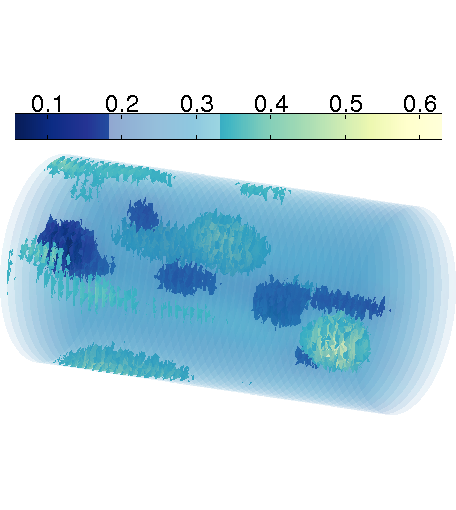


The algorithm then proceeds in the standard way, i.e., with the simultaneous reconstruction of the absorption and the diffusion; see steps 1–4 in Algorithm 1. The residuals for both the outer and the inner iteration are depicted in Figure 5. The algorithm terminates after five linearisations (including step 0), meaning that the reconstruction, presented in Figure 6, is a result of four linearisations of the measurement model (cf. step 4 of Algorithm 1). The reconstructions of both optical parameters are in accordance with the prior information: there are well localised inclusions in an approximately constant background. Moreover, the inclusions lie at approximately correct positions. On the negative side, the reconstruction of the diffusion exhibits some instability near the object boundary, which causes very high jumps at a few isolated nodes: the highest and the lowest point values are and , respectively. However, discarding the nodes at the boundary, one gets the reasonable extremal values and (which are used as the limits for the diffusion plot in Figure 6). In addition, in spite of the aforementioned outliers in the reconstructed diffusion, the mean values over the background and the inclusions presented in Table 2 are approximately correct for both parameters. Even though the reconstructed means are not exactly the same as the target values, they are very close to the corresponding mean values of the interpolated parameters and (except for the ‘most difficult’ diffusive inclusion (1) lying along the axis of ), which is arguably the best one can expect to achieve.
As mentioned after Algorithm 1, the reconstructions seem insensitive to the choice of the threshold parameter . Considering significantly higher noise levels (say, 10%) clearly deteriorates the quality of the reconstructions, with the diffusion coefficient exhibiting a higher level of instability. However, e.g., doubling the noise level does not considerably alter the performance of the algorithm. Moderate changes in the density of the reconstruction mesh mainly affect the reconstruction process via the computation time.
The running time of Algorithm 1 for this experiment was approximately minutes with a MATLAB (2014a) implementation on a laptop with GB RAM and an Intel Core i7-4600U CPU having clock speed GHz.
| Absorption | mean values () | Diffusion | mean values (mm) | ||||
|---|---|---|---|---|---|---|---|
| bg | 0.01 | 0.0101 | 0.00996 | bg | 0.3 | 0.300 | 0.304 |
| (1) | 0.05 | 0.0459 | 0.0456 | (1) | 0.05 | 0.0874 | 0.0708 |
| (2) | 0.02 | 0.0189 | 0.0188 | (2) | 0.05 | 0.0668 | 0.0628 |
| (3) | 0.002 | 0.00266 | 0.00263 | (3) | 0.15 | 0.163 | 0.165 |
| (4) | 0.05 | 0.0432 | 0.0425 | (4) | 0.6 | 0.579 | 0.595 |
| (5) | 0.002 | 0.00338 | 0.00335 | (5) | 0.05 | 0.0792 | 0.0764 |
| (6) | 0.15 | 0.169 | 0.174 | ||||
| (7) | 0.6 | 0.573 | 0.576 | ||||
Test 2
In practical applications it is not always possible to illuminate the target from several different directions. We next study the effect of the number and position of illuminations on the cubical target of size visualised in Figure 7(a). The absorption is composed of a homogeneous background with two embedded inhomogeneities: a cross-shaped inclusion lying along the plane with absorption and an origin-centered spherical shell with outer radius , inner radius and the absorption level (except at the intersection with the cross). The background diffusion level is and there are also two diffusive inhomogeneities: a cross-shaped inclusion lying along the plane with diffusion and a ball centered at the origin with radius and diffusion (except at the intersection with the cross).
To begin with, we illuminate the object through its bottom face with only one photon flux that is modeled as the characteristic function
where . The simulation of the data follows the same steps as in the previous example; in particular, the level of additive noise is still one percent. (In this case, the fine FE mesh has nodes and tetrahedrons whereas the coarse one has nodes and tetrahedrons.)


Using the same free parameters and forming the initial guesses and as in the first example, we get the approximate background levels and as well as the final reconstruction presented in Figure 7(b). The reconstruction of the absorption is reasonable, although it includes shadows of the diffusive inclusions. On the other hand, the diffusion produced by Algorithm 1 is almost constant, making it practically useless. This reconstruction, resulting in a (nonlinear) residual clearly under the noise level , was obtained after only two steps of LSQR already in step 0 of the algorithm. The reconstructions one gets by starting with , i.e., without step 0, or even by setting are essentially the same. In addition, changing the direction of the illumination does not seem to affect the results. We conclude that when using only one illumination, the absorption can explain the measurement (almost) completely, and hence one cannot simultaneously reconstruct the diffusion. This is not very surprising as it is well known that the optical inverse problem of QPAT is nonunique for one illumination; see [4, 13, 31, 37, 44]. However, to add an extra twist, [7] recently presented a uniqueness result for piecewise constant absorption and diffusion with only one illumination.
Let us then complement the measurement corresponding to the flux with a second one. To evaluate the effect of the chosen illumination directions, we consider two cases: illuminations through adjacent faces and through opposite sides. To study the first case, we combine with , i.e., a homogeneous flux through the right-hand face of the cube. In the second case, is accompanied by , i.e., a homogeneous flux through the top facet. Both and are modelled by the appropriate characteristic functions on . The reconstruction algorithm is run for the two cases with the same free parameters as previously. As a result, we get the same approximate background values as with one illumination, but the final reconstructions, presented in Figures 7(c)–7(d), are significantly better: two illuminations result in decent reconstructions of both optical parameters. It has to be noted, however, that the directions of the two employed photon fluxes play a significant role: for the illuminations through adjacent faces, the reconstructed diffusion is inaccurate close to the opposite edge, whereas the opposite illuminations lead to good quality reconstructions of both parameters in the whole domain.
Finally, we add a third measurement to the two-illumination settings considered above. The additional measurement is induced by a homogeneous photon flux through the back of the cube, with its amplitude modelled once again by the appropriate characteristic function. The triplet , and corresponds to illuminations around one corner of the cube, while the facet-wise fluxes , and for the other three-illumination test cover the boundary of the cube as evenly as possible. The resulting reconstructions are presented in Figures 7(e)–7(f). Compared to the two-illumination cases, the reconstructions of the diffusion are now somewhat sharper. However, as with two adjacent illuminations, when the three photon fluxes are supported around one corner, the reconstruction of the diffusion close to the opposite corner is far from satisfactory. For three illuminations, there should be no problem with the (theoretical) uniqueness, so it seems that the physics of the measurement setting limits the reconstruction quality: the light does not penetrate deep enough into the object in order to provide reliable information about the diffusion near the opposite corner, where the reconstruction mainly reflects the prior information. On the other hand, complementing the opposite illuminations with a third measurement leads to slightly more detailed reconstructions, but the difference between the two- and three-illumination cases is not substantial (cf. Figures 7(d) and 7(f)).
The reconstructions corresponding to two illuminations shown in Figures 7(c)–7(d) resulted from three linearisations of the measurement model in Algorithm 1 (including step 0), while it took four linearisations to produce the three-illumination reconstructions in Figures 7(e)–7(f). The corresponding computation times were about five and ten minutes, respectively, with the same hardware as in Test 1.
6 Concluding remarks
In this work, the inverse problem of QPAT was investigated. The aim of QPAT is to produce high-resolution reconstructions of the optical parameters of interest from given three-dimensional, high-resolution PAT images. A computationally efficient algorithm for the inverse problem of QPAT was introduced by combining priorconditioned LSQR, a lagged diffusivity step and linearisations of the measurement model in two nested iterations. To facilitate handling a high number of measurements and unknowns, all multiplications by Jacobians in the algorithm were implemented in a matrix-free manner. The numerical studies exclusively employed a Perona–Malik prior, although other types of edge-preserving priors can as easily be utilised in the described approach. The proposed reconstruction algorithm was tested with 3D numerical simulations. The results demonstrate that the approach is capable of producing accurate and good quality estimates of the absorption and diffusion in complex 3D geometries in a reasonable computation time, even when the tests are run on a standard laptop. This suggests that QPAT can be developed into a practical method without compromising the accuracy of the estimates or the good resolution the method can potentially provide.
Appendix: Matrix-free approximation of the Jacobians
The aim of this appendix is explaining how to efficiently approximate multiplications by the Jacobian of the map
where is the discretisation of the measurement , cf. (7), and
are the elementwise transformations of the parameters introduced in (4). As in Sections 3 and 4, we only consider here the case of one illumination, which corresponds to the photon flux , cf. (1). In the case of multiple illuminations, more bookkeeping of the indices is required, but otherwise the described methodology works as for a single flux of photons.
First of all, since and for all , we get the Jacobian by the chain rule
In particular, operating with boils, in essence, down to multiplying with .
According to Lemma 1, the Fréchet derivative of is
where is the solution of (1) and is the solution of the variational problem (3). To approximate at the optical parameters and corresponding to given and , we use the FEM with the piecewise linear basis appearing in (5) to evaluate , letting the perturbations and run in turns through . To be more precise, denoting the node values of the FEM approximations for , and by , and , respectively, we approximate
where
Accordingly, the (approximate) Jacobian is formed as
We still need to consider how to handle multiplications by and matrix-freely.
Based on the weak formulation of (1),
we first form the FEM system matrix and load vector corresponding to the basis , and solve the node values from the equation
Next, we approximate the derivative based on the variational problem (3). Since the left-hand side of (3) is identical to that in the weak formulation of (1), the FEM system matrix stays the same. Letting the perturbations on the right-hand side of (3) run in turns through , we get the load matrix and the equation
where
for .
Finally, instead of solving the huge system to form the Jacobian explicitly, we use the matrices and to implicitly operate on a given vector: multiplying by gives
We also need to be able to multiply a given vector with the transpose . Since matrices and are symmetric, we get
Numerically speaking, multiplying a vector by the Jacobian or its transpose is relatively cheap: one only needs to perform elementwise multiplications of vectors and matrix-vector multiplications with sparse matrices, and to operate with the inverse of the FEM system matrix on a vector. However, when the number of degrees of freedom and/or illuminations is very high, the sizes of the matrices and may become impractically large. In this case, one can continue the analysis to avoid forming the matrices and altogether, but the details are omitted here for brevity.
References
- [1] Alberti, G. S., and Ammari, H. Disjoint sparsity for signal separation and applications to hybrid inverse problems in medical imaging. Appl. Comput. Harmon. Anal. (2015). In Press.
- [2] Arridge, S., Betcke, M., and Harhanen, L. Iterated preconditioned LSQR method for inverse problems on unstructured grids. Inverse Problems 30 (2014), 075009.
- [3] Arridge, S. R. Optical tomography in medical imaging. Inverse Problems 15 (1999), R41–R93.
- [4] Bal, G., and Ren, K. Multi-source quantitative photoacoustic tomography in a diffusive regime. Inverse Problems 27 (2011), 075003.
- [5] Bal, G., and Ren, K. On multi-spectral quantitative photoacoustic tomography in a diffusive regime. Inverse Problems 28 (2012), 025010.
- [6] Beard, P. Biomedical photoacoustic imaging. Interface Focus 1 (2011), 602–631.
- [7] Beretta, E., Muszkieta, M., Naetar, W., and Scherzer, O. A variational method for quantitative photoacoustic tomography with piecewise constant coefficients. arXiv:1509.04982 (2015).
- [8] Calvetti, D. Preconditioned iterative methods for linear discrete ill-posed problems from a Bayesian inversion perspective. J. Comput. Appl. Math. 198 (2007), 378–395.
- [9] Calvetti, D., McGivney, D., and Somersalo, E. Left and right preconditioning for electrical impedance tomography with structural information. Inverse Problems 28 (2012), 055015.
- [10] Calvetti, D., and Somersalo, E. Priorconditioners for linear systems. Inverse problems 21 (2005), 1397–1418.
- [11] Calvetti, D., and Somersalo, E. Hypermodels in the Bayesian imaging framework. Inverse Problems 24 (2008), 034013.
- [12] Cox, B., Laufer, J. G., Arridge, S. R., and Beard, P. C. Quantitative spectroscopic photoacoustic imaging: a review. J. Biomed. Opt. 17 (2012), 061202.
- [13] Cox, B. T., R., S., Arridge, and Beard, P. C. Estimating chromophore distributions from multiwavelength photoacoustic images. J. Opt. Soc. Am. A 26 (2009), 443–455.
- [14] Dierkes, T., Dorn, O., Natterer, F., Palamodov, V., and Sielschott, H. Fréchet derivatives for some bilinear inverse problems. SIAM J. Appl. Math. 62 (2002), 2092–2113.
- [15] Ding, T., Ren, K., and Vallélian, S. A one-step reconstruction algorithm for quantitative photoacoustic imaging. Inverse Problems 31 (2015), 095005.
- [16] Eldén, L. A weighted pseudoinverse, generalized singular values, and constrained least squares problem. BIT 22 (1982), 487–502.
- [17] Gao, H., Feng, J., and Song, L. Limited-view multi-source quantitative photoacoustic tomography. Inverse Problems 31 (2015), 065004.
- [18] Gao, H., Osher, S., and Zhao, H. Quantitative photoacoustic tomography. In Mathematical Modeling in Biomedical Imaging II, H. Ammari, Ed. Springer, 2012, pp. 131–158.
- [19] Gao, H., Zhao, H., and Osher, S. Bregman methods in quantitative photoacoustic tomography. UCLA CAM Report 10-42 (2010).
- [20] Grisvard, P. Elliptic Problems in Nonsmooth Domains. Pitman, 1985.
- [21] Haltmeier, M., Neumann, L., and Rabanser, S. Single-stage reconstruction algorithm for quantitative photoacoustic tomography. Inverse Problems 31 (2015), 065005.
- [22] Hannukainen, A., Harhanen, L., Hyvönen, N., and Majander, H. Edge-promoting reconstruction of absorption and diffusivity in optical tomography. Inverse Problems 32 (2016), 015008.
- [23] Hansen, P. C. Rank-Deficient and Discrete Ill-Posed Problems. SIAM, 1998.
- [24] Harhanen, L., Hyvönen, N., Majander, H., and Staboulis, S. Edge-enhancing reconstruction algorithm for three-dimensional electrical impedance tomography. SIAM J. Sci. Comput. 37 (2015), B60–B78.
- [25] Hilgers, J. W. On the equivalence of regularization and certain reproducing kernel Hilbert space approaches for solving first kind problems. SIAM J. Numer. Anal. 13 (1976), 172–184.
- [26] Kaipio, J. P., and Somersalo, E. Statistical and Computational Inverse Problems. Springer–Verlag, 2005.
- [27] Kuchment, P., and Kunyansky, L. Mathematics of thermoacoustic tomography. Eur. J. Appl. Math. 19 (2008), 191–224.
- [28] Laufer, J., Cox, B., Zhang, E., and Beard, P. Quantitative determination of chromophore concentrations form 2D photoacoustic images using a nonlinear model-based inversion scheme. Appl. Opt. 49 (2010), 1219–1233.
- [29] Li, C., and Wang, L. V. Photoacoustic tomography and sensing in biomedicine. Phys. Med. Biol. 54 (2009), R59–R97.
- [30] Mamonov, A. V., and Ren, K. Quantitative photoacoustic imaging in radiative transport regime. Comm. Math. Sci 12 (2014), 201–234.
- [31] Naetar, W., and Scherzer, O. Quantitative photoacoustic tomography with piecewise constant material parameters. SIAM J. Imaging Sci. 7 (2014), 1755–1774.
- [32] Paige, C. C., and Saunders, M. A. Algorithm 583: LSQR: Sparse linear equations and least squares problems. ACM Trans. Math. Softw. 8 (1982), 195–209.
- [33] Paige, C. C., and Saunders, M. A. LSQR: An algorithm for sparse linear equations and sparse least squares. ACM Trans. Math. Softw. 8 (1982), 43–71.
- [34] Perona, P., and Malik, J. Scale-space and edge detection using anisotropic diffusion. IEEE Trans. Pattern Anal. 12 (1990), 629–639.
- [35] Pulkkinen, A., Cox, B. T., Arridge, S. R., Kaipio, J. P., and Tarvainen, T. Direct estimation of optical parameters from photoacoustic time series in quantitative photoacoustic tomography. Submitted.
- [36] Pulkkinen, A., Cox, B. T., Arridge, S. R., Kaipio, J. P., and Tarvainen, T. A Bayesian approach to spectral quantitative photoacoustic tomography. Inverse Problems 30 (2014), 065012.
- [37] Pulkkinen, A., Cox, B. T., Arridge, S. R., Kaipio, J. P., and Tarvainen, T. Quantitative photoacoustic tomography using illuminations from a single direction. J. Biomed. Opt. 20 (2015), 036015.
- [38] Pulkkinen, A., Kolehmainen, V., Kaipio, J. P., Cox, B. T., Arridge, S. R., and Tarvainen, T. Approximate marginalization of unknown scattering in quantitative photoacoustic tomography. Inverse Probl. Imag. 8 (2014), 811–829.
- [39] Razansky, D., Baeten, J., and Ntziachristos, V. Sensitivity of molecular target detection by multispectral optoacoustic tomography (MSOT). Med. Phys. 36 (2009), 939–945.
- [40] Ren, K., Gao, H., and Zhao, H. A hybrid reconstruction method for quantitative PAT. SIAM J. Imaging. Sci. 6 (2013), 32–55.
- [41] Rudin, L. I., Osher, S., and Fatemi, E. Nonlinear total variation based noise removal algorithms. Physica D 60 (1992), 259–268.
- [42] Saratoon, T., Tarvainen, T., Arridge, S. R., and Cox, B. T. 3D quantitative photoacoustic tomography using the -Eddington approximation. In Proc. of SPIE (2013), A. A. Oraevsky and L. V. Wang, Eds., vol. 8581, pp. 85810V–1.
- [43] Saratoon, T., Tarvainen, T., Cox, B. T., and Arridge, S. R. A gradient-based method for quantitative photoacoustic tomography using the radiative transfer equation. Inverse Problems 29 (2013), 075006.
- [44] Shao, P., Cox, B., and Zemp, R. Estimating optical absorption, scattering and Grueneisen distributions with multiple-illumination photoacoustic tomography. Appl. Opt. 50 (2011), 3145–3154.
- [45] Shao, P., Harrison, T., and Zemp, R. J. Iterative algorithm for multiple illumination photoacoustic tomography (MIPAT) using ultrasound channel data. Biomed. Opt. Express 3 (2012), 3240–3248.
- [46] Song, N., Deumié, C., and Silva, A. D. Considering sources and detectors distributions for quantitative photoacoustic tomography. Biomed. Opt. Express 5 (2014), 3960–3974.
- [47] Tarvainen, T., Cox, B. T., Kaipio, J. P., and Arridge, S. R. Reconstructing absorption and scattering distributions in quantitative photoacoustic tomography. Inverse Problems 28 (2012), 084009.
- [48] Tarvainen, T., Pulkkinen, A., Cox, B. T., Kaipio, J. P., and Arridge, S. R. Bayesian image reconstruction in quantitative photoacoustic tomography. IEEE Trans. Med. Imag. 32 (2013), 2287–2298.
- [49] Vogel, C. R., and Oman, M. E. Iterative methods for total variation denoising. SIAM J. Sci. Comput. 17 (1996), 227–238.
- [50] Wang, L. V., Ed. Photoacoustic Imaging and Spectroscopy. CRC Press, 2009.
- [51] Xu, M., and Wang, L. V. Photoacoustic imaging in biomedicine. Rev. Sci. Instrum. 77 (2006), 041101.
- [52] Zemp, R. J. Quantitative photoacoustic tomography with multiple optical sources. Appl. Opt. 49 (2010), 3566–3572.