Crustal Failure on Icy Moons from a Strong Tidal Encounter
Abstract
Close tidal encounters among large planetesimals and moons should have been more common than grazing or normal impacts. Using a mass spring model within an N-body simulation, we simulate the deformation of the surface of an elastic spherical body caused by a close parabolic tidal encounter with a body that has similar mass as that of the primary body. Such an encounter can induce sufficient stress on the surface to cause brittle failure of an icy crust and simulated fractures can extend a large fraction of the radius of body. Strong tidal encounters may be responsible for the formation of long graben complexes and chasmata in ancient terrain of icy moons such as Dione, Tethys, Ariel and Charon.
Keywords: Tides, solid body: Satellites, surfaces:
1 Introduction
A number of large surface features in the solar system have origins potentially due to giant impacts that occurred between planet-sized bodies or planets and large planetesimals. These include the crustal dichotomy of Mars (Wilhelms & Squyres, 1984; Frey & Schultz, 1988; Marinova et al., 2008) and the Moon (Jutzi & Asphaug, 2011), jumbled terrain on Mercury (Schultz & Gault, 1975) and numerous impact craters throughout the solar system (Melosh, 1989). Because of their larger cross-section, grazing impacts among planets and planetesimals are more likely than normal angle impacts (Asphaug, 2010). Likewise, strong tidal encounters, those involving close encounters between two large bodies that do not actually touch, are more likely than grazing impacts. A fraction of a body’s gravitational binding energy can be dissipated during a close tidal encounter (Press & Teukolsky, 1977). While some large surface features on planets and moons have proposed origins due to large impacts, so far none have been linked to single close and strong tidal encounters.
Strong tidal encounters are unlikely now, but would have occurred in the past, during the late-heavy bombardment era and beforehand. Orbits of closely packed moons can become unstable (e.g., French & Showalter 2012; Cheng et al. 2014) and this too could cause close encounters between similar mass bodies. Impacts primarily cause compressive stress (Melosh, 1989), but tidal stress can be tensile and many materials are weaker when subjected to tensile stress than a comparable magnitude of compressive stress (for ice see Figure 1 by Petrovic 2003 and Figure 7.2 by Collins et al. 2010 and for the Earth’s lithosphere see failure envelopes in Figure 6.24 and Yield Strength envelopes in Figure 6.27 by Watts 2001 or Figure 9.6 by Kohlstedt & Mackwell 2010). Ancient regions of planets and moons exhibit features such as chasmata, grooves, grabens or graben complexes that are associated with extension and tensile deformation (Collins et al., 2010), and some of these may have been caused by strong tidal encounters with large bodies.
Many studies of tidal encounters between two planetesimals or between a planetesimal and a planet have focused on tidal disruption (e.g., Dobrovolskis 1990; Boss 1994; Richardson et al. 1998; Sharma et al. 2006; Holsapple & Michel 2008). But tidal stresses due to close encounters between bodies can affect body rotation and shape (Bottke et al., 1999) and disturb weathered surfaces of asteroids, exposing fresh surface materials (Binzel et al., 2010; Nesvorny et al., 2010). Simulations of granular materials have predicted resurfacing in weak regions where tidal stresses cause avalanches or landslides (Yu et al., 2014).
Some icy moons exhibit global tectonic features, such as grooves or long fractures, that could be caused by varying tidal stresses exerted by their host planet (e.g., Helfenstein & Parmentier 1985; McEwen 1986; Hurford et al. 2007; Smith-Konter & Pappalardo 2008; Wahr et al. 2009; Hurford et al. 2015). The patterns and individual morphologies of parallel sets of grooves and troughs on satellites and asteroids such as Phobos, Eros, Ida, Gaspra, Epimetheus and Pandora (see Thomas & Prockter 2010 for a review) can be attributed to fracturing in weak materials caused by oscillating tidal stresses associated with orbital eccentricity (Morrison et al., 2009) or an increase in tidal stress resulting from the orbital decay of the body itself (Soter & Harris, 1977; Hurford et al., 2015). For Phobos, the length of the grooves is perpendicular to the oscillating tensile stress (Morrison et al., 2009). Long (130 km) linear fractures termed “tiger stripes” on Enceladus are connected to diurnal tidal stress variations (Smith-Konter & Pappalardo, 2008; Nimmo & Matsuyama, 2007; Hurford et al., 2007).
Dione, Tethys, Rhea (moons of Saturn), Titania (moon of Uranus) and Charon (moon of Pluto) have heavily cratered surfaces and also display long faults extending a significant fraction of the moon radius, and chasma and faults in pairs interpreted as graben or graben complexes (for a review see section 6.4 by Collins et al. 2010 and for recent results on the Pluto system see Stern et al. 2015). The Ithaca Chasma on Tethys is interpreted to be a large graben complex (Giese et al., 2007) and crater counts indicate that it is older than the large Odysseus impact basin (with radius 0.4 times that of the moon itself). On Dione, Cassini imagery revealed that some fault networks have vertical offsets that dissect craters, confirming their extensional tectonic origin and suggesting that they were formed early (Jaumann et al., 2009). These studies suggest that the formation of chasmata and graben complexes can take place before or during an epoch of large impacts and so during an epoch when strong tidal encounters would have occurred. Explanations for the graben complexes include heating and expansion of the interior (e.g., Hillier & Squyres 1991) and stresses induced by reorientation following a large impact (Nimmo & Matsuyama, 2007). Strong tidal encounters have not yet been explored as a possible explanation for the formation of surface features such as chasmata and graben complexes on icy moons.
In this study we focus on the intersection between the works introduced above. We consider rare and close tidal encounters, that might have occurred billions of years ago, between large bodies that are not gravitationally bound (not in orbit about each other). The time of a parabolic or hyperbolic tidal encounter can be a few hours, so tidal encounters are extremely fast compared to the time scales of most geophysical processes. On such a short time scale rock and ice should deform in a brittle-elastic mode rather than a ductile, plastic or visco-elastic mode (e.g., Turcotte & Schubert 2002; Br̈ugmann & Dresen 2008). To numerically simulate tidal deformation we use a mass-spring model to simulate both elastic response and gravity (see Frouard et al. 2016). Brittle failure is modeled by allowing springs on the surface to fail if they exceed a critical tensile strain value. Our simulations allow to us to visualize brittle crustal failure following a hypothetical strong tidal encounter. Our approach differs from the granular flow simulations by Schwartz et al. (2013) with spring-like forces between neighboring soft spheres that mimic cohesion and can simulate bulk tensile failure.
1.1 Tidal encounters
Following Press & Teukolsky (1977) (also see Ogilvie 2014) the response of a body during a tidal encounter can be estimated using an impulse approximation. The maximum tidal force, , on body from body during the encounter is approximately
| (1) |
where is the distance between body centers at closest approach (pericenter), is the mass of the tidal perturber, is the radius of the primary body with mass , and is the gravitational constant. The time scale of the encounter is
| (2) |
where is the velocity at pericenter. Together and cause a velocity perturbation on the surface of the primary body
| (3) |
If the orbit is parabolic then , a dimensionless parameter used to characterize parabolic tidal encounters (Press & Teukolsky, 1977), that is the ratio of acceleration due to self-gravity and the tidal acceleration at the body’s surface.
The extent of the tidal deformation of body can be estimated by balancing the kinetic energy per unit mass due to the tidal impulse with elastic energy per unit mass
| (4) |
with the Young’s modulus and the density of body , giving a strain of
| (5) |
where
| (6) |
is the velocity of a particle in a circular orbit grazing the surface of and
| (7) | |||||
is approximately the gravitational binding energy density of body (and to order of magnitude its central pressure). We have assumed that is a homogenous and spherical body and remains so during the encounter.
A time scale for elastic response can be estimated from the speed of elastic waves and the radius of the primary body.
| (8) |
where we have defined a gravitational time scale
| (9) | |||||
equivalent to the the inverse of the angular rotation rate of a particle in a circular orbit grazing the surface of the body . The gravitational time scale is only dependent on the body’s mean density . For a Poisson modulus of , the speed for P-waves is and that for S waves . To order of magnitude is equal to the frequency of the slowest vibrational mode of the body.
The strain rate (on ) during the tidal encounter can be estimated from the time scale for elastic response
| (10) | |||||
This expression implies that close encounters between similar mass bodies are likely to be in a high strain rate regime (geophysical strain rates tend to be 10 orders of magnitude lower, see Figure 2 by Hammond et al. 2013, Nimmo 2004b and discussion below).
The above estimate for the strain and strain rate used an impulse approximation, assuming that the body does not have time to elastically respond during the encounter. We compare the elastic response time scale to the encounter time scale
| (11) |
If then the impulse approximation is valid, whereas if the encounter can be considered adiabatic. When the ratio of time scales is near unity, the impulse approximation can be used but the response should be reduced by a factor that depends on the ratio of the two time scales.
In Table 1 we list gravitational energy densities , time scales and densities for some moons that exhibit long faults, chasmata or graben complexes. The planet Mars, which exhibits the extremely prominent chasm, Valles Marineris, is included for later discussion. The gravitational time scales in the icy bodies range from about 1000-2000 s (15 to 30 minutes). We compare the gravitational binding energy densities, , to an estimate for the Young’s modulus of ice. Observations of ice shelf response to tides on Earth give an effective Young’s modulus GPa (Vaughan, 1995), an order of magnitude below that of solid ice in the lab. On icy moons, porosity and surface fracturing may lower the effective value of the Young’s modulus (Nimmo & Schenk 2006; see Collins et al. 2010 for a review). The values of gravitational energy density for icy bodies in Table 1 range from 0.3 GPa for Tethys to 2.14 for Titania. Depending upon the value adopted for the Young’s modulus for ice, the ratio ranges from about 1 to 0.1 for these bodies.
Using the estimate for the ratio we estimate the strain during an encounter. For an equal mass and density perturber, the pericenter distance must be more than twice the body’s radius; . For a parabolic grazing encounter with , the pericenter velocity is equal to the escape velocity at pericenter, and with defined in equation 6. Equation 5 then implies that the strain caused by the tidal encounter could be of order 10% for a parabolic equal mass encounter. The ratio is large enough that the time scale for the encounter could be a few times longer than the elastic time scale. This should reduce the strain on the surface compared to that estimated using the impulse approximation in equation 5 by a factor of a few (with factor that depends on the ratio ). Icy moons are likely to contain rocky higher density and strength cores and here we have neglected compositional variation in our estimate of the tidally induced surface strain. This too would reduce the estimated strain value by a factor of a few. Nevertheless our low estimated ratio of implies that icy crusts or mantles in these icy bodies are weak enough that deformation at the level of few percent strain is expected in close parabolic tidal encounters with similar mass objects.
Close encounters with a similar mass body would be in a regime of high strain rate, compared to most geophysical settings for ice, but lie in the mid to lower end of laboratory measurements (Lange & Ahrens, 1993; Schulson, 1999; Fortt & Schulson, 2012). Figure 2 by Petrovic (2003) illustrates that the tensile strength of ice is relatively insensitive to the strain rate, however Lange & Ahrens (1993) found a dependence, with the strength increasing at very high strain rates. At strain rates of order the tensile strength of ice is a few MPa (Lange & Ahrens, 1993; Schulson, 1999; Petrovic, 2003). Using a Young’s modulus of a few GPa, brittle failure is likely to take place if the strain under uniaxial tension exceeds 0.01 - 0.1%. This crude strain based estimate for brittle failure ignores a dependence of the material strength on depth or pressure. One of the modes of tensile failure causes fractures parallel to one of the axes of principal stress and is independent of confining pressure (Jaeger & Cook, 1976). This is equivalent to the limit with principal stress (as on the body’s surface), , corresponding to extension, and the Griffiths failure criterion that is a function only of the uniaxial tensile strength. Here fractures are expected parallel to the direction associated with (on the surface and perpendicular to the principal axis of tensile stress). Based on our estimate of the induced strain during a close encounter with a massive body (equation 5) and using the values for gravitational energy density for the icy bodies listed in Table 1, we estimate that tidal stress and associated body deformation could cause sufficient tension on the surfaces of these bodies to exceed the tensile strength of their icy crusts and cause widespread surface brittle failure.
| mass | radius | ||||
|---|---|---|---|---|---|
| ( kg) | (km) | (GPa) | (s) | g cm-3 | |
| Tethys | 0.62 | 531 | 0.32 | 1906 | 0.98 |
| Dione | 1.1 | 561 | 0.81 | 1556 | 1.48 |
| Rhea | 2.3 | 764 | 1.04 | 1701 | 1.24 |
| Ariel | 1.3 | 579 | 1.08 | 1468 | 1.66 |
| Titania | 3.5 | 788 | 2.14 | 1443 | 1.72 |
| Charon | 1.5 | 603 | 1.16 | 1472 | 1.65 |
| Mars | 642 | 3389 | 208 | 953 | 3.93 |
2 Mass-Spring Model Simulations
Because of the short time scale of tidal encounters we model brittle-elastic behavior alone and neglect ductile, plastic or liquid-like behavior. We model only the tidal encounter, and do not model longer time scale viscoelastic behavior, such as crustal flexure, subsidence and decompression melting. Mass-spring models or lattice spring models are a popular method for simulating soft elastic bodies (Meier et al., 2005; Nealen et al., 2006). In a mass-spring model, massive particles are connected with a network of massless springs. Mass-spring models are considered a better choice than a finite difference method when a fast, but not necessarily accurate simulation is desired. However, with enough masses and springs and an appropriate choice of spring types, behaviors and geometry for the network of connections, mass spring models can accurately represent elastic materials (Hrennikoff, 1941; Monette & Anderson, 1994; Ostoja-Starzewski, 2002; Clavet et al., 2005; Kot et al., 2015). Tidal spin down of spherical bodies can accurately be modeled with a random mass-spring model (Frouard et al., 2016).
Our simulations differ from those used to model granular materials (e.g., Richardson et al. 2009; Richardson et al. 2011; Schwartz et al. 2013). We apply gravitational, elastic and damping forces to pairs of particles with the direction of force parallel to the vector connecting the pair. In contrast in simulated granular materials, particles that touch can exert a torque on each other. In a mass-spring model ductile and plastic behavior is only possible if spring rest lengths can vary or if springs can dissolve and reform (e.g., Clavet et al. 2005). In contrast, simulated granular materials can flow like a strengthless incompressible fluid (e.g., Leinhardt et al. 2012).
To study crustal deformation we need to numerically resolve the surface with a moderate number of surface particles. The spherical surface is supported by the interior of the body and feels stresses due to deformation of the interior. We model the surface using a regular 2-dimensional triangular lattice of masses. The lattice structure allows us to track and render the surface. We model the interior with randomly distributed more widely spaced and more massive particles than used in the surface shell.
Most mass-spring models do not take into account the self-gravity of the body itself. Our mass-spring model is embedded inside an N-body code and so takes into account gravitational forces between all particles in the body itself as well as the perturbing body. To carry out our simulations we use the modular code rebound, an open-source multi-purpose N-body code for collisional dynamics (Rein & Liu, 2012) (available at http://github.com/hannorein/). From the rebound version 1 code (from June 2015), we use the open-GL display, open boundary conditions, the direct all pairs gravitational force computation and the leap-frog integrator (second order and symplectic) to advance particle positions. To the particle accelerations we have added additional spring and hinge forces, as described below. We have modified the display to illustrate the springs between particles and add textures to the surface layer.
We work in units of the planetesimal body radius and mass . Time is specified in units of (equation 9) and we refer to this as a gravitational time scale. In these units, the velocity of a particle in a circular orbit just grazing the surface of the body is , and the period of this orbit is . Velocities are given in units of , accelerations in units of and spring constants in units of . Pressure, energy density and elastic moduli are given in units of or (equation 7). In units of the mean density of the primary body is .
The parameters used to describe our simulations are summarized in Table 2.
2.1 Spring forces
The code rebound advances particle positions using their accelerations (Rein & Liu, 2012). We add spring and hinge forces as additional forces by adding to the particle accelerations at each time step. To compute the particle accelerations, the forces from each spring and hinge on each particle are divided by the mass of each particle.
The elastic force from a spring between two particles with masses and coordinate positions , , on particle is computed as follows. The vector between the two particles gives a spring length that we compare with the spring rest length . The elastic force from a spring between two particles on particle is computed as
| (12) |
where is the spring constant and the unit vector . The force has the opposite sign on particle . When the spring length is longer than its rest length the force pulls the two masses together and when it is shorter than its rest length the force pushes the two masses apart.
The strain rate of the spring is
| (13) |
where and are the particle velocities, is the rate of change of the spring length, and is the spring strain. To the elastic force on particle we add a damping force proportional to the strain rate
| (14) |
with damping coefficient that is equivalent to the inverse of a damping or relaxation time scale. The coefficient is independent of the spring constant . Here is the reduced mass . The damping force is in parallel with the elastic term so the spring model approximates a viscously damped elastic material or a Kelvin-Voigt solid (see Frouard et al. 2016). Between each pair of particles, forces are oriented along the vector spanning the two particles and this ensures angular momentum conservation.
To maintain numerical stability, the time step should be smaller than the time it takes physical information to travel between adjacent mass nodes. The ratio of the P-wave velocity to gravitational velocity and this exceeds 1 otherwise the body would collapse due to self-gravity. In our simulations the speed of elastic waves exceeds so we must choose the time step to be shorter than the time it takes for elastic waves to propagate between adjacent mass nodes;
| (15) |
taking the minimum value of all springs in the model and with factor the number of springs per node.
2.2 Random isotropic mass-spring model for the interior
We generate an isotropic random mass-spring model for the interior similar to the random spring model described by Kot et al. (2015). Each mass is a node and all nodes in the interior have the same mass. Random particle positions are generated but a particle is added to the network only if it is sufficiently separated from other nodes (at a distance greater than minimum distance ). Springs are added between two nodes if the distance between nodes is less than distance . Such a spring network is isotropic, has Poisson ratio and has a Young’s modulus of
| (16) |
(Kot et al., 2015), where and are the spring constants and spring rest lengths for spring , and is the total volume. In the above expression the sum is over all springs in the interior volume.
We compute the velocity of waves in the interior with
| (17) |
With non-zero damping coefficients, the stress is the sum of an elastic term proportional to the strain and a viscous term proportional to the strain rate. The bulk and shear viscosities can be estimated from the damping coefficient, , and other integrated properties of the mass spring model (Frouard et al., 2016).
In a three-dimensional volume, the number of springs is proportional to the number of particles in the interior, . The mean length of the springs giving spring constant to maintain a specific Young’s modulus. The mass of each particle is . Altogether this gives a time step (using equation 15) and, as expected, the more particles simulated, the smaller is the required time step. (Frouard et al., 2016) has tested sensitivity of the random spring model to numbers of simulated mass nodes and numbers of springs per node.
2.3 Initial conditions for the interior: Stretching the springs and strengthening the core
We first generate springs with rest length equal to the distance between the spring vertices. However this does not generate an equilibrium state for our body because of compression due to self-gravity. When the simulation is begun in this state the body shrinks and then bounces, eventually damping to a denser equilibrium state than the initial condition. To begin with the system nearer equilibrium we start with the springs initially slightly under compression so that they counter-act self-gravity. We iteratively stretch all springs by the same amount to zero the acceleration at the surface. We then increase the spring strengths in the center of the body so as to approximate a state of hydrostatic equilibrium. A constant density self-gravitating sphere in hydrostatic equilibrium has pressure as a function of radius
| (18) |
(consistent with equation 2 by Dobrovolskis 1990). The pressure at any radius is approximately where is the strain of each spring. The resulting model is nearly in equilibrium, nearly constant density, and does not bounce excessively at the beginning of the simulation.
To illustrate the elasticity of the interior we show a gravitational tidal encounter with a perturber mass , equal to the primary body, . The simulation is shown in Figure 1 and has body parameters listed in Table 3 and encounter parameters listed in Table 4 under the row N. The perturbing mass, , is modeled as a solid sphere that does not deform during the encounter and it is rendered as a sphere with the same density as the primary body. The simulation view has been shifted so that it remains in the center of mass frame of the primary body. As the spring damping coefficient is low, the body is soft, like jello and the body continues to vibrate and deform after the tidal encounter. Vibrational oscillations are excited in the body by the tidal encounter. We have checked that the elasticity code conserves momentum and angular momentum, as would be expected as particle interaction forces (including damping forces) are radial.11 1 The difference between angular momentum at the beginning and end of the simulation is less than in our N-body units described in section 2.0. With the resolved body in a circular orbit about a larger mass and on long time scales, the spring damping causes the resolved body to spin up or spin down, as expected, and with rate matching that predicted analytically (Frouard et al., 2016).

2.4 Crustal Shell Model
We model the elastic crust with a 2-dimensional spherical lattice. Each vertex of the shell lattice is a mass node and each node has the same mass. However the shell node masses are not the same as the interior node masses. To create a sphere of particles we begin with vertices of an icosahedron. Each face is then subdivided into 4 triangles. We recursively repeat this operation until we reach a desired total number of vertices in the shell, . Each vertex is the same distance from the body center. After subdivision, springs are placed with spring constant between each adjacent vertex, creating a triangular spring lattice (see Figure 2) and giving the 2-dimensional shell elasticity (e.g. Monette & Anderson 1994; Van Gelder 1998). The vertices of each triangular face are stored to later aid in displaying (rendering) the body’s surface.
For a triangular 2D lattice, the Young’s modulus depends on the spring constant
| (19) |
and the Poisson ratio is (see equations 3.7 by Monette & Anderson 1994 or equations 10,12 by Kot et al. 2015). The modulus is a force per unit length rather than a force per unit area as is true in 3D. The sphere locally contains a single layer of particles and approximates a thin plate with
| (20) |
where is the Young’s modulus of the plate and its thickness. For particles in the shell, the mean length of the springs , the mass of each particle but is independent of the number of particles. Hence the required time step (using equation 15) . The speed of P-waves in the shell is
| (21) |
where is the mass per unit area in the shell.
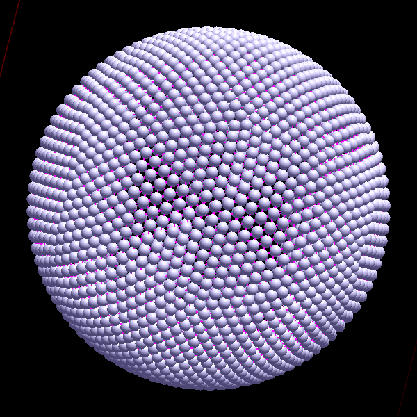
2.5 Hinge Forces and Flexure of the Crustal Shell
As a 2-dimensional lattice is used to simulate the body’s crust, the simulated crust is a thin membrane and when simulated with radial elastic forces between particles, and in the presence of gravity, it would be unstable and would bend and sag. Using the triangular phases in our crustal sphere, we use a hinge model to resist bending of adjacent triangular faces.
The force on each edge depends on the dihedral angle between the two faces as described by Bridson et al. (2003) in their section 4, see Figure 3, also see Grindspun et al. (2003). An angular dependent force is applied to the two vertices in a spring edge and to two adjacent vertices forming the hinge. The magnitude of the applied force is
| (22) |
where is the length of the edge. The dihedral angle is equivalent to with angle between the two vectors, and , that are normal to the surfaces of each triangular face. Here and are the areas of the two triangular faces of the hinge (see Figure 3). The force strengths are the same on each vertex but applied with direction given in vector form given by Bridson et al. (2003) assuring momentum and angular momentum conservation. The angle is a rest bend angle and describes the angle of the surface without stress. We adjust the sign of by ordering the vertices in the edge. Before the simulation starts for each hinge we compute from the initial configuration of the surface lattice. Here our surface lattice is spherical but rest hinge angles can be computed for any smooth 2-dimensional lattice. This ensures that the initial state of our simulated crustal shell is not under flexural stress. As is true for the spring forces, accelerations for each mass are computed from the applied forces by dividing by the mass of each vertex particle.
The coefficient is in units of force but the force is applied at each hinge and with opposite sign in the center and ends of the hinge. The hinge is similar to a flexed beam, held at both ends but with an applied force at its center, and with width equal to the length of the hinge edge and length equal to the distance between outer vertices. The hinge model locally approximates a thin plate with Young’s modulus and plate thickness with
| (23) |
with the length of an edge and equal to the flexural rigidity or bending stiffness of the plate (e.g., Batty et al. 2012). This is approximate as simulated static load tests have not been carried out with the membrane/hinge model (though simulated static beam tests have been done for the lattice and random spring models, see Kot et al. 2015).

2.6 Crack formation
Crack formation in the crustal shell can be simulated in a spring model by breaking springs that have a strain value above a critical threshold value, , (e.g., Norton et al. 1991; Marder & Liu 1993; Hirota et al. 2000; Sadhukhan et al. 2011). The springs in our simulated spherical shell behave as perfect linear springs until the moment that they reach the threshold value. If we completely dissolve failed springs, eventually three particles in a hinge triangle face (see Figure 3) could approach a line. When this happens the hinge force (equation 22) becomes infinite and the surface is unstable. Rather than completely dissolve springs, we instead reduce the spring force constant by a factor .
When a crack forms in a solid, the stress perpendicular to the crack’s path is reduced. Subsequent deformation concentrates stress at the new crack tip, which in turn fails, allowing the crack to propagate. In a simulation, the stress is redistributed as vertex positions are updated, and this allows the crack to propagate. A simple way to allow the stress redistribution (or relaxation) to take place within the simulation is to allow only only one element to rupture in a given time interval, often the simulation time step (see discussion by Pfaff et al. 2014). Here, we only allow a single shell spring, that with maximum strain, to fail in a given time interval, denoted , which we set between one and three time steps. This relaxation procedure allows linear fractures to propagate, and prevents large areas of the surface from failing simultaneously. A more sophisticated code would allow more than one crack to simultaneously propagate (and in this case additional relaxation steps must be implemented and the residual momentum propagation taken into account in each crack tip region; Busaryev et al. 2013; Pfaff et al. 2014).
The surface of the shell is displayed using the triangular faces from each lattice triangle. Each triangular face is displayed with a texture. The edges of each triangle contain connecting springs. The texture displayed on each triangular face depends on the number and orientations of failed edge springs (see Figure 4). Long connected or partially connected sets of black bars illustrate surface fractures. The surface lattice introduces directional biases in the crack rendering. Offset individual black bars in Figure 4 are artifacts from the lattice rather than en-echelon structures.

2.7 Support of the Shell
The crustal shell lattice must be supported by the interior otherwise it will collapse due to gravity. To connect the two components of our models (amorphous interior to the lattice shell membrane) we insert springs between shell particles and interior particles. We create springs for all mixed pairs of particles, a pair consisting of a particle in shell and a particle in the interior, that have inter-particle distance less than a distance . The springs that cross between the interior and shell, we denote cross springs and they are described with a spring constant , number and mean rest length . The number of cross springs per shell particle can be increased by increasing the distance .
To ensure that the initial model does not bounce excessively at the beginning of the simulation, these springs are initially set slightly under compression, as described in section 2.3. An illustration of our cross springs is shown in Figure 5.
We match the speed of elastic waves traveling horizontally in the shell to the speed of vertical oscillations of the cross springs. The strength of the cross springs we estimate using the dimensional scaling of equation 16
| (24) |
where the Young’s modulus is that of the interior and the value for spring constant depends on the number of cross springs per shell particle. Compression is communicated elastically from the crust to the interior with a speed
| (25) |
where is the mass in the shell. We adjust and so that the coupling speed is comparable to the velocity of P-waves in the interior, .

2.8 Damping to an equilibrium state
If the crustal shell is initially under compression at the beginning of the simulation, increased extension would be needed to cause spring failure. If there are local crustal stresses present at the beginning of the simulation, they would influence the location of tensile failure during the tidal encounter. Despite adjustment of interior spring lengths and strengths (described in section 2.3), and setting the cross springs slightly under compression, the body bounces radially at the beginning of a simulation. This can affect the timing (and so location) of crustal tensile failure, as failure would be most likely to occur when the body has largest radius. We would like shell springs to be at their rest lengths at the beginning of the simulation and the body should be in equilibrium and not vibrating. To ensure equilibrium and zero the stress in the crust we run a relaxation simulation before each tidal encounter. The relaxation simulations are run without a tidal perturber, of the primary body alone, with a large damping parameter . During this relaxation simulation, springs are not allowed to fail and we slowly adjust the lengths of the shell springs so that they approach a zero force condition. The rest hinge angles are periodically reset to zero the flexural stress of the surface.
At the end of the relaxation, shell springs are very close to their rest lengths (under no extension or compression), the vibrations of the body have decayed, and the crustal membrane is under no flexural stress. The support of the crustal membrane by compression by the cross springs approximates hydrostatic support even though there is no density contrast. The relaxation simulations are run (in units of the gravitational time scale; equation 9) under a damping coefficient (for all springs) of . After the relaxation run is finished we store the positions and velocities of all masses and properties of all springs and hinges so that they can be read back into the code to run the tidal encounters. By simulating the relaxed body with a low damping coefficient and without an encounter, we check that the body is stable and that springs do not fail in the absence of any perturber.
2.9 Parameter choices for the Tidal encounters
To describe the primary body a large number of parameters must be chosen (see Table 2). We adjusted the minimum distance distance between particles to be somewhat larger than the distance between shell particles as we need to well resolve the shell but not the interior. The parameter was adjusted so that the number of springs per node in the interior exceeded 10, and so that the effective elastic coefficients (Young’s modulus and Poisson ratio) are not strongly dependent on the spring network (Kot et al., 2015). The shell mass and distance between shell and outer boundary of the interior were adjusted to give the shell approximately the same density as the interior and so that implied shell thickness is approximately consistent with that estimated from the flexural strength and speed of elastic waves through the crust.
The spring constant in the interior was chosen so that the Young’s modulus of the interior is approximately 3, matching an estimate for the value of ice’s Young’s modulus in units of for the icy bodies listed in Table 1. We adjusted spring constants in the cross springs and shell so that the speed of elastic waves in the shell is similar to that in the interior and the speed of vibrations passing from shell to cross spring and assumed composition of crust and interior is similar. The spring constant in the shell was adjusted so that the implied crustal thickness from equation 20 gave (in units of radius), corresponding to 10 km crustal thickness for a body with of radius km. Estimates for the thickness of the icy crust on Dione and Tethys range from 1 - 7 km, and are based on assuming that topographic features are signatures of flexure of a broken elastic plate (Giese et al., 2007; Hammond et al., 2013). Our modeled thickness exceeds these estimates by a factor of 2–3 but they are based on flexure over long time scales (Myr) and the effective elastic thickness of the crust should be larger on the shorter tidal time scale (hours). A comparison of observed and predicted flexural rigidity (proportional to effective thickness to the third power) as a function of age of geological load for seamounts and oceanic islands implies that elastic thickness is a strong function of strain rate (see section 6.7 by Watts 2001) but it would be inaccurate to extrapolate over orders of magnitude to tidal time scales. Our simulated crustal shell is connected via cross springs to the interior so vibrational waves can propagate throughout the body, similar to the way seismic waves propagate through the Earth’s mantle. Using the implied crustal thickness, , a flexural force parameter, , was chosen to be stronger than that estimated using equation 23) so as to maintain numerical stability (keep the hinges from collapsing) during the simulation.
The strain value for surface spring failure for most of the simulations was chosen to be , however weaker tidal encounters would allow the surface to fracture were we to reduce this number. The strength reduction parameter (setting spring strength after failure in a shell spring) was set high enough to ensure that surface triangles never collapsed to a line during the simulation. Collapse of a surface triangle causes the surface to become numerically unstable as the hinge forces become infinite when the triangular face areas drop to zero.
After the relaxation runs are done, we run the tidal encounters. During the encounter simulations no new springs are created and only shell springs are allowed to fail. The tidal encounter simulations are begun and ended with the secondary mass located at distance of approximately 3 times the radius of the primary away from the primary body center and are run for a total time of in gravitational units. The perturber is modeled as a point mass. The inverse of our gravitational time unit is equivalent to the spin of a body with surface near the centrifugal rotational breakup velocity. Most moons rotate much more slowly than this value (e.g., Murray & Dermott 1999). As tidal encounters are fast (taking place on a time ), we ignore the role of the spin of the primary body, setting it to zero. Gravitational softening is set to 1/100 of the minimum initial inter-particle spacing and we have checked that its exact value does not influence the simulations. Simulations were run at half the timestep listed in Table 3 to check that the resulting surface morphologies were similar and not dependent on the time step.
| Number of particles in interior | |
| Number of interconnecting springs in interior | |
| Mean rest spring length in interior | |
| Mean spring constant of interior springs | |
| Young’s modulus of interior | |
| Interior spring formation distance | |
| Minimum initial interparticle distance | |
| Speed of P-waves in the interior | |
| Number of particles in shell | |
| Number of interconnecting springs in shell | |
| Mass of shell | |
| Mean rest spring length of shell springs | |
| Spring constant of shell springs | |
| Bending spring constant for flexural strength of shell | |
| Simulated crustal thickness | |
| Maximum strain for spring failure in shell | |
| Factor spring constant is reduced after spring failure | |
| Speed of P-waves in the shell | |
| Number of cross springs connecting shell and interior | |
| Mean rest spring length of cross springs | |
| Spring constant of cross springs | |
| Cross spring formation distance | |
| Effective velocity of shell and interior coupling | |
| Spring damping coefficient | |
| Time step | |
| Time interval between failure of individual springs | |
| Mass of tidal perturber | |
| Distance between body centers at closest approach | |
| Relative velocity at closest approach |
The first group of parameters describes the random elastic interior (Section 2.2). The second group describes the shell lattice (section 2.4 and 2.5. The third group describes the cross springs connecting shell to interior (section 2.7). The fourth group lists damping coefficient for all springs and the time step used in the integrations. The last group lists properties of the tidal encounter. The Young’s modulus is computed using equation 16. Lengths are in units of the body’s initial radius. Timescales are in units of the gravitational time scale (equation 9). Masses are in units of the body’s mass. Moduli are in units of (the body’s gravitational binding energy, equation 7). The spring damping coefficient is in units of inverse time. Effective shell plate thickness is estimated using equation 23 or 20. Velocities are computed using equations 17, 21, 25.
| N | T-series | |
| 798 | 1869 | |
| 11632 | 23363 | |
| 0.30 | 0.176 | |
| 0.0076 | 0.076 | |
| 0.4 | 3.73 | |
| 0.38 | 0.10 | |
| 0.15 | 0.23 | |
| 1.4 | 4.5 | |
| 0 | 2562 | |
| 7680 | ||
| 0.07 | ||
| 0.075 | ||
| 0.06 | ||
| 0.0075 | ||
| 0.02 | ||
| 0.003 | ||
| 0.005 | ||
| 3.28 | ||
| 0 | 5966 | |
| 0.156 | ||
| 0.005 | ||
| 0.18 | ||
| 3.3 | ||
| 0.1 | 0.01 | |
| 0.003 | 0.002 | |
| - | 3 |
Interior particle positions were randomly generated individually for each simulation and have slightly different numbers of interior particles, interior and cross springs and from those listed here. The T1 simulation has a slightly lower .
| Simulation | Description | |||
|---|---|---|---|---|
| N | 1.0 | 2.13 | 1.84 | interior only |
| T5 | 0.5 | 1.84 | 1.60 | fiducial |
| T1 | 0.1 | 1.47 | 1.62 | lower mass perturber and weaker crust |
| T10 | 1.0 | 2.10 | 1.61 | higher mass perturber |
| T10b | 1.0 | 2.22 | 1.94 | higher mass perturber and faster encounter |


3 Fractures from Simulated Strong Tidal Encounters
We illustrate four tidal encounters with body parameters listed in Table 3 under the column T-series and with encounter parameters listed in Table 4. The T5 simulation has perturber , half the mass of the primary body. The T1 simulation has a lower strain failure parameter allowing crustal failure with a lower mass perturber, . The T10, T10b simulations have an equal mass perturbers and the T10b encounter is faster than the T10 encounter.
The morphology of the simulated fractures are shown in Figure 6 using an orthographic projection, and showing an entire hemisphere. In these figures, the tidal perturber passes from right to left in the plane perpendicular to the line of sight. For each simulation, four panels are shown at different times in the simulation, advancing from the leftmost to the rightmost panel. Pericenter occurs with perturber almost directly in front of the primary body and blocking our view of it. We render the secondary body with the same density as the primary body and as nearly transparent so that the surface of the primary body can still be seen. The trajectories of the perturbing body with respect to our resolved body at different times in the orbit and in the orbital plane are shown in Figure 7 for the same tidal encounter simulations shown in Figure 6 and listed in Table 3. The resolved body, modeled with the mass-spring network, is shown as a black circle at the origin. The viewer for the snapshots shown in figure 6 is located at at negative in Figure 7 and looking upwards. Open circles illustrate the locations of the perturbing body for the snapshots shown in Figure 6 and has radius set from its mass and assuming that it has the same density as the resolved body. Even though the perturber is modeled as a point mass, we show a radius for the perturber so that the reader has a feeling for the proximity of the two bodies during the tidal encounter. If the perturbing body has a similar density as the primary, these are nearly grazing encounters.
Using the orbital plane to define an equatorial plane for the body, the surfaces after the encounters are shown in Figure 8 in a cylindrical projection (horizontal axis corresponding to longitude and vertical axis showing latitude) for the same simulations. In these figures with longitude ranging from to the subsatellite point (point of closest approach during the encounter) lies on the equator at a longitude of and on the right hand side.
Figure 6 shows that simulated crustal fractures extend a large fraction of the body, even for the lowest mass perturber. Cracks are oriented both perpendicular and parallel to the orbit path, and are predominantly present on a single hemisphere (see Figure 8). Cracks tend to be concentric around the point of closest approach (also called the subsatellite point). As expected, the faster encounter T10b causes fewer fractures but the fractures seem to cover the same extent. For only the lowest mass perturber are the fractures confined to nearer the subsatellite point.
 |
 |
 |
 |
Our simulations produce crude illustrations of surface fractures that we can compare to long chasmata or graben complexes on icy bodies such as those listed in Table 1. In Figure 9 we show full hemispheres using an orthographic projection of Dione, Tethys and Charon created from maps available from the The Jet Propulsion Lab Photojournal (see http://photojournal.jpl.nasa.gov/). The images shown in Figure 9 were made using the open-GL display software Sphere-Mapper (https://github.com/dmgiannel/Sphere-Mapper), written by one of us (David Giannella), that takes cylindrical projection cartographic maps and applies them as a texture to a sphere that can be tilted to any desired angle and rotation angle and viewed using an orthographic projection. The Dione input image is the Planetary Image Atlas (PIA) 18434 that is a global 3-Color map of Dione (IR-Green-UV) posted April 2014. Its cartographic control and digital mosaic construction are by Dr. Paul Schenk (LPI, Houston). The original map has a simple cylindrical map projection at 250m/pixel at equator and is based on Cassini ISS images acquired 2004-2014. The global map of Saturn’s moon Tethys (PIA 11673) was created using images taken by NASA’s Cassini spacecraft and includes new data collected during Cassini’s Aug. 14, 2010, flyby (original Image Credit: NASA/JPL/Space Science Institute). The map of Charon we used (PIA 19866) is by NASA/Johns Hopkins University Applied Physics Laboratory/Southwest Research Institute and was created from all available resolved images of the surface acquired between July 7-14, 2015, at pixel resolutions ranging from 40 kilometers on the anti-Pluto facing hemisphere (left and right sides of the map), to 400 meters per pixel on portions of the Pluto-facing hemisphere.
The fractures we have simulated (Figures 6, 8) are of similar extent to those exhibited by the bodies shown in Figure 9. However our simulated bodies often exhibit more than one large fracture, and only Dione has as many chasmata. Dione has a number of large chasmata, but they are not concentric about a single point as seen on our simulated fractured bodies. The C shaped feature on Dione known as Padua Chasmata, shown on the top left in Figure 9, might originate from a very close but lower mass encounter with closest approach at the center of the C. Ithaca Chasma on Tethys, as a single set of features, might be consistent with a fracture caused by a lower mass perturber (1/10 of that of Tethys) or more distant encounter with a massive perturber (equal mass). The long sequence of chasmata on Charon forming a great arc (Macross and Serenity chasmata)22 2 Names of features on Charon are still informal. might have been caused by a moderately distant encounter with a very large object, such as Pluto itself. Our simulations do show parallel sets of fractures (for example in the T10 simulation) that might correspond to a series of parallel chasmata such as Tardis and Nostromo Chasmata that are parallel to Macross and Serenity Chasmata on Charon.
3.1 Discussion
Within the bright terrain on Ganymede is a mosaic of ridges and troughs, termed grooved terrain, exhibiting abundant evidence of extensional strain (e.g., see Pappalardo & Greeley 1995 and Collins et al. 2010 section 6.1.2). Ganymede has a higher energy density, GPa, than the icy bodies we listed in Table 1, and this lies in between the Young’s modulus of ice (a few GPa) and rocky materials 50– 100 GPa. If Ganymede were approximated with an elastic solid with Young’s modulus similar to materials in the Earth’s lithosphere, GPa, then equation 5 suggests that a near equal mass perturber tidal encounter would crack Ganymede’s surface. Due to Ganymede’s liquid metal core and its few hundred km deep subsurface saltwater ocean (e.g., Saur et al. 2015), Ganymede would deform more strongly to a tidal encounter than a purely elastic body. Ganymede is differentiated so a model with a multiple layer interior, comprised of both solids and liquids, is required to study its tidal response.
We have taken care in our simulations to relax the body before each encounter and we have tried to model a crust with constant thickness, uniform elasticity and flexural rigidity that is approximately hydrostatically supported. Even though we have used a moderate number of particles to resolve shell and interior, the random particle distribution of the interior and associated spring network is not even. There are different numbers of cross springs per shell particle so some areas of the surface shell are more likely to fail than others and this prevents us from running at low levels of maximal strain . Conversely icy crust on moons is unlikely to have uniform thickness and composition and could be under residual localized stress. Our simulations predict symmetrical features above and below the orbital plane, but real bodies are likely to be heterogeneous in terms of crustal thickness, thermal state and pre-existing fractures so they might preferentially fracture in weaker regions and only on one side. Here we have neglected body spin. However with a nearly parabolic (or slow) encounter with a rapidly spinning body (near the breakup spin rate), tidal stresses on the surface would not be symmetrical and this too could cause asymmetry in the fracture distribution.
We found that our simulated bodies did not exhibit fractures for encounters with larger pericenter distances or higher encounter velocities. The escape velocity from Dione is km/s and this is representative for the escape velocities for the other icy bodies listed in Table 1. In comparison, the orbital velocity of Dione is approximately 10 km/s and the orbital velocity of Saturn is 9.6 km/s. This implies that tidal encounters with asteroids or centaurs would preferentially be at higher relative velocities with ratio and so higher than the parabolic encounters consider here (see equation 5 for the estimated strain dependence on encounter velocity). However, encounters with moons that are also orbiting the planet would have much lower relative velocities. The orbital speed of Charon is only 0.2 km/s so an encounter between Charon and Pluto would have been in the nearly parabolic regime simulated here. While a fast encounter from an external object would be isolated, if a close tidal encounter occurs between two satellites orbiting the same body, then multiple close encounters are likely, each producing a group of fractures about a different pericenter locus.
Vibrations are excited during a tidal encounter and vibrational energy dissipated due to the viscoelastic body response and surface fracture. The total energy dissipated should be a small fraction (at most a few percent) of the gravitational binding energy (Press & Teukolsky, 1977) and so is at most a small fraction of the orbital energy. Only if the encounter is almost exactly parabolic would this energy loss allow the two bodies to become gravitational bound (in orbit about each other) after the encounter.
Here we have modeled the perturbing body as a point mass. If this body is a strong solid and nearly spherical this is a good approximation. However if the perturbing body were weak (a low cohesion rubble pile, e.g., Richardson et al. 2009) and lower mass than the primary body then it could be strongly deformed or disrupted during then encounter and its tidal field would significantly differ from that of a point mass.
Many large icy moons are believed to have global oceans which decouple the motions of their floating shells from their interiors (Schubert et al., 2004; Thomas et al., 2016) and these could make the tidal response larger than estimated from elasticity of a solid body alone (e.g., Iess et al. 2012). Conversely, in our simulations we have neglected the presence of a rocky core and this would have reduced the tidal response compared to that simulated here using a uniform body. The maximum strain value for spring failure for most of our simulations may be an over estimate for the brittle strength of ice, so faster and more distant tidal encounters might also be able to cause crustal fractures in icy satellites. Unfortunately we cannot yet run simulations with lower levels of because the surfaces tend to exhibit fractures even in the absence of a perturber. We have also been unable to run encounters with larger mass bodies because in this regime, the shell can be lifted off the body, our surface triangles collapse and the hinge forces cause the shell to become unstable (and explode). So far we have only simulated elastic materials and do not have the capability to simulate simultaneously elastic and liquid materials, though we could increase the density and strength in the core by adjusting particle masses and spring constants so we could mimic the behavior of a rocky core. We would like to improve our code to improve its precision and extend the types of materials that we can simulate.
We have briefly explored the effect of a non-linear spring force law on the cross springs by multiplying the spring forces (equation 12) by a strain dependent factor (Clavet et al., 2005)
| (26) |
where sets a strain scale and the spring force is reduced as this scale is approached. Here is a factor that limits the minimum force under extension so that it never drops to zero. However for the strengths of the bodies we have simulated here, and using the same initial relaxed body, we saw little difference in simulated fracture morphology when we varied from 0.02 to 0.04 (and the maximum strain value was never approached, possibly because the cross springs begin under compression). Were we to simulate a weaker (so thinner) surface, a reduction in the connection of the surface to the interior would affect simulated fracture extent and morphology.
Lithospheric brittle failure depends on depth, tensile mode, strain and strain rate (see the review by Burov 2011). Here we have adopted a simplistic maximal strain value for brittle failure. Crack propagation is only crudely simulated here, and crack morphology is numerically dependent on the nature of relaxation and so here on the time interval used to identify failed springs in the simulation. When this interval is reduced (and comparing simulations beginning with the same relaxed body), there is some additional surface failure and in some regions wider cracks can form. To meaningfully predict fault lengths, widths and structures we would need to better simulate crack formation, propagation, decompression and subsequent relaxation. Wholesale crustal failure in a model with more realistic coupling between crust and interior might exhibit fluid flow from subsurface oceans and decompression melting.
We have not seen qualitative differences in fracture morphology if we set rest lengths of springs to their failure length when they fail. For the strongest perturber (the T10) simulation large regions of the surface were ruptured. If crack propagation were more accurately modeled with higher resolution, these might manifest as jumbled terrain or parallel sets of fractures and graben complexes.
Here we have only simulated brittle elastic response. At the high strain rates of tidal encounters there must be a depth where the ice is ductile and deforms plastically. If we more accurately modeled the strength envelope and material properties as a function of depth, then fractures would open during the encounter but they would not close all the way afterwards, giving us an estimate for their extension.
We have not modeled viscoelastic response on long time scales. While we might have identified regions where fractures originate, our work does not predict depths and widths of resulting chasmata or graben complexes that might result. Improved simulations would more accurately model crack propagation, fracture formation and explore the subsequent evolution of the resulting geophysical structures, such as magna and water escape along dilatant cracks and associated partial resurfacing.
3.1.1 Cracking Mars’ Lithosphere
Using the Young’s modulus of a rocky material, 50-100 GPa, we notice that Mars has ratio of gravitational energy density to Young’s modulus 2–4, only a factor of a few higher than estimated for the icy bodies we have listed in Table 1. The yield strength envelope as a function of depth for a rocky lithosphere reaches a maximum at about a few hundred MPa (e.g., Figure 6.35 by Watts 2001). The maximum strength divided by a Young’s modulus of 50 GPa (for a rocky material) gives a ratio of order 0.01, similar to the value of maximal strain for uniaxial tensile brittle failure of ice that we used above as a criterion to mimic fracture in an icy crust. The ratio and the maximum uniaxial strain for crustal brittle failure are similar for icy moons and Mars, suggesting that that the scenario we have explored here can be scaled to Mars. If Mars experienced a strong (nearly equal mass) and close tidal encounter with a rocky body, tensile deformation during the encounter could have fractured Mars’ lithosphere.
Valles Marineris is thought to have been formed by crustal extension (Tanaka and Golombek, 1989) similar to the formation of rift faults like the East African Rift (Eginber et al., 1991). Valles Marineris was formed after much of the volcanic Tharsis bulge or rise was in place (see section 4.5 by Golombek and Phillips 2010). Tectonic formation scenarios for Valles Marineris associate its formation with the inability of Mars’ lithosphere to support the large load of the Tharsis bulge itself (Tanaka and Golombek, 1989; Mège and Masson, 1996; Nimmo & Tanaka, 2005; Golombek and Phillips, 2010; Andrews-Hanna, 2012a; Andrews-Hanna, 2012b; Andrews-Hanna, 2012c). Flexural (bending and membrane) stresses in the lithosphere account for the radial grabens on the topographic rise and concentric compression wrinkle ridges around its circumference (Banerdt & Golombek, 2000; Golombek and Phillips, 2010). However, a stress model that is azimuthally symmetric about the center of the Tharsis rise would predict radial grabens that are of similar length and width on opposite sides of the rise. In contrast, Valles Marineris (south east of the peak) is exceptional – much wider and deeper than radial grabens to the north or west of the center of the rise.
Gravity and topography data indicate that Mars’ crustal thickness is bimodal, approximately 30 km in the northern hemisphere and 60 km in the souther hemisphere, and exceeding 80 km on the Tharsis bulge (Neumann et al., 2004). Andrews-Hanna (2012b) proposed that Valles Marineris is located near and aligned with the buried crustal dichotomy boundary that bisects the Tharsis bulge. In his model, the difference in crustal thickness underlying the Tharsis bulge generates tensile stress directly along the crustal dichotomy boundary and this accounts for the exceptional width and depth of Valles Marineris compared to other radial grabens surrounding the Tharsis bulge.
We have found that a strong tidal encounter can cause long extensional fractures that extend a significant fraction of the body’s radius. So a tidal encounter might account for the exceptional depth and length of Valles Marineris. However, we expect (see Figure 8) fractures in a large ring centered at the point of closest approach. If a tidal encounter were responsible for formation of Valles Marineris why doesn’t the valley extend further, forming a large ring? We simulated a relaxed, constant thickness, uniform elasticity and flexural rigidity crustal shell but Mars’ lithosphere is not uniform thickness and has variations in levels of localized stress. During a tidal encounter, Mars’ lithosphere could have preferentially fractured along a region of localized stress rather than in a circle centering the point of closest approach. Magma underlying the Tharsis bulge at the time of the tidal encounter may have allowed Mars’ crust to be more easily deformed during the encounter, perhaps even lifted away from the core. So the volcanic activity in the Tharsis province itself could have exacerbated tidal deformation. A tidal encounter is an intriguing alternate explanation for the extensional stress forming Valles Marineris, but a more sophisticated study would be needed to test it and contrast it with tectonic models for the formation of Valles Marineris.
4 Summary and Additional Discussion
In this paper we have explored tidal encounters with elastic bodies using a mass-spring model to simulate elasticity within the context of an N-body simulation. We have simulated crustal failure using an elastic shell model, with flexural stiffness for the crust. Brittle failure is modeled using a maximum strain value for the surface springs, and crack propagation modeled with a crude relaxation procedure, allowing only a single spring to fail in a specific time interval (a few computational time steps). Our simulations illustrate that strong, close tidal encounters can cause crustal failure on icy bodies, confirming an order of magnitude estimate for the tidally induced surface strain. Following the encounters, simulated crustal shells exhibit long fractures extending over a large fraction of a body radius. Using near parabolic encounters with a nearly equal mass body perturbing a non-spinning body, we find that surface fractures tend to be concentric around the subsatellite point (point of closest approach for the encounter) and are restricted to a single hemisphere. Tidally induced crustal fractures might provide an explanation for long chasmata and graben complexes on icy bodies such as Dione, Tethys and Charon.
We have attempted to construct simulations that represent icy bodies. However, the tidal regime, because it is at high strain rate, is different than other geophysical settings (such as studies of crustal plate flexure). If some chasmata are explained by tidal encounters we might be able to place constraints on the effective crustal elastic thickness at high strain rate and on the connection between crust and interior. Conversely uncertainty in the rheological models make it difficult for us to carry out simulations accurate enough to do this comparison.
We have focused here on icy bodies that have old crusts. Rocky satellites and asteroids such as Phobos, Eros, Ida, Gaspra, Epimetheus and Pandora can exhibit long grooves and troughs (see the review by Thomas & Prockter 2010). Single tidal encounters could be investigated as a mechanism for the formation of fractures that are suspected to underly their surface regolith. Lastly, strong close tidal encounters might have occurred with large rocky bodies such as Mars, and old regions of their surfaces may retain extensional features caused by these encounters.
Acknowledgements We thank Maciej Kot, Moumita Das, Julien Frouard, Stephen Burns, Alexander Moore, Melissa Morris, April Russel, Matt Hedman, Hanno Rein, Rob French, Matt Tiscareno, and Shoshanna Cole for encouraging and helpful discussions. This work was in part supported by NASA grant NNX13AI27G.
References
- Aggarwal & Oberbeck (1974) Aggarwal, H.R., Oberbeck, V.R., 1974. Roche limit of a solid body. Astrophysical Journal, 191, 577-588.
- Andrews-Hanna (2012a) Andrews-Hanna, J.C., 2012a. The formation of Valles Marineris: 1. Tectonic architecture and the relative roles of extension and subsidence. J. Geophys. Res., 117, E03006.
- Andrews-Hanna (2012b) Andrews-Hanna, J. C., 2012b. The formation of Valles Marineris: 2. Stress focusing along the buried dichotomy boundary. J. Geophys. Res., 117, I E04009.
- Andrews-Hanna (2012c) Andrews-Hanna, J. C., 2012c. The formation of Valles Marineris: 3. Trough formation through super-isostasy, stress, sedimentation, and subsidence. J. Geophys. Res., 117, E06002.
- Asphaug (2010) Asphaug, E., 2010. Similar-sized collisions and the diversity of planets. Chemie der Erde, 70, 199-219.
- Banerdt & Golombek (2000) Banerdt, W. B., Golombek, M. P., 2000. Tectonics of the Tharsis region of Mars: Insights from MGS topography and gravity (abs.). Lunar Planet. Sci. Conf. XXXI, 2038, Houston, TX: Lunar and Planetary Institute (CD-ROM).
- Batty et al. (2012) Batty, C., Uribe, A., Audoly, B., Grindspun, E., 2012. Discrete Viscous Sheets. ACM Transactions on Graphics (Proceedings of SIGGRAPH 2012), 31, 113:1-113:7.
- Baudet et al. (2009) Baudet, V., Beuve, M., Jaillet, F., Shariat, B., Zara, F., 2009. Integrating Tensile Parameters in Mass-Spring Systems for Deformable Object Simulation. Technical Report Rapport Recherche LIRIS, RR-LIRIS-2009-034, LIRIS UMR 5205 CNRS/INSA de Lyon/Université.
- Binzel et al. (2010) Binzel, R. P., Morbidelli, A., Merouane, S., DeMeo, F. E., Birlan, M., Vernazza, P., Thomas, C. A., Rivkin, A. S., Bus, S. J., Tokunaga, A. T., 2010. Earth encounters as the origin of fresh surfaces on near-Earth asteroids. Nature, 463, 331-334.
- Bridson et al. (2003) Bridson, R., Marino, S., Fedkiw, R., 2003. Simulation of Clothing with Folds and Wrinkles. In: Breen, D., Lin, M. (Eds), Proceedings of the 2003 ACM SIGGRAPH/Eurographics symposium on Computer animation, pp. 28-36.
- Boss (1994) Boss, A.P., 1994. Tidal disruptions of periodic Comet Shoemaker-Levy 9 and a constraint on its mass density. Icarus, 107, 422-426.
- Bottke et al. (1999) Bottke, W. F., Richardson, D. C., Michel, P., Love, S. G., 1999. 1620 Geographos and 433 Eros: Shaped by Planetary Tides? Astronomical Journal, 117, 1921-1928.
- Br̈ugmann & Dresen (2008) Bürgmann, R., Dresen, G., 2008. Rheology of the Lower Crust and Upper Mantle: Evidence from Rock Mechanics, Geodesy, and Field Observations. Annual Review of Earth and Planetary Sciences, 36, 531-56.
- Burov (2011) Burov, E. B., 2011. Rheology and strength of the lithosphere. Marine and Petroleum Geology, 28, 1402-1443.
- Busaryev et al. (2013) Busaryev, O., Dey, T. K., Wang, H., 2013. Adaptive fracture simulation of multi-layered thin plates. ACM Transactions on Graphics (SIGGRAPH 2013 Proceedings), 32, no. 4, pp. 52:1–52:6.
- Cheng et al. (2014) Cheng, W. H., Peale, S. J., & Lee, M. H. 2014. On the origin of Pluto’s small satellites by resonant transport Icarus, 241, 180-189.
- Clavet et al. (2005) Clavet, S., Beaudoin, P., Poulin, P., 2005. Particle-based Viscoelastic Fluid Simulation. In: Anjyo, K., Faloutsos, P.(Eds.), Proceedings of the 2005 ACM SIGGRAPH/Eurographics symposium on Computer animation, pp. 219-228.
- Collins et al. (2010) Collins, G. C., McKinnon, W. B., Moore, J. M., Nimmo, F., Pappalardo, R. T., Prockter L. M., Schenk, P. M., 2010. Tectonics of the outer planet satellites. In: Watters, T. R., Richard A. Schultz, R. A. (Eds.), Planetary Tectonics, Cambridge University Press, Cambridge England, pp. 264-350.
- Dobrovolskis (1990) Dobrovolskis, A.R., 1990. Tidal disruption of solid bodies. Icarus 88, 24-38.
- Eginber et al. (1991) Ebinger, C. J., Karner, G. D. Weissel, J. K., 1991. Mechanical strength of extended continental lithosphere: Constraints from the western rift system, East Africa. Tectonics, 10, 1239-1256.
- Fortt & Schulson (2012) Fortt, A. L., Schulson E. M., 2012. Friction of ice on ice. J. Geophys. Res., 117, B12204.
- French & Showalter (2012) French, R. S., Showalter, M. R., 2012. Cupid is Doomed: An Analysis of the Stability of the Inner Uranian Satellites, Icarus, 220, 911-921.
- Frey & Schultz (1988) Frey, H., Schultz, R. A., 1988. Large impact basins and the mega-impact origin for the crustal dichotomy on Mars. Geophys. Res. Lett., 15, 229-232.
- Frouard et al. (2016) Frouard, J., Quillen, A.C., Gianella, D., Efroimsky, M., 2016. Numerical Simulation of Tidal Evolution of a Viscoelastic Body Modeled with a Mass-Spring Network. Monthly Notices of the Royal Astronomical Society, 458, 2890 - 2901.
- Giese et al. (2007) Giese, B., Wagner, R., Neukum, G., Helfenstein, P., Thomas, P. C., 2007. Tethys: Lithospheric thickness and heat flux from flexurally supported topography at Ithaca Chasma. Geophys. Res. Lett., 34, L21203-L21207.
- Golombek and Phillips (2010) Golombek, M. P., Phillips, R. J., 2010, Mars Tectonics, In: Watters, T. R., Schultz, R. A. (Eds.), Planetary Tectonics, Cambridge University Press, Cambridge England, pp. 183-232.
- Grindspun et al. (2003) Grindpun, E., Hirani, A. N., Schröder, P., Desbrun, M. 2003. Discrete shells. In: Breen, D., Lin, M. (Eds), Proceedings of the 2003 ACM SIGGRAPH/Eurographics symposium on Computer animation, pp. 62-67.
- Hammond et al. (2013) Hammond, N. P., Phillips, C. B., Nimmo, F., Kattenhorn, S. A., 2013. Flexure on Dione: Investigating subsurface structure and thermal history. Icarus, 223, 418-422.
- Helfenstein & Parmentier (1985) Helfenstein, P., Parmentier, E. M.,1985. Patterns of fracture and tidal stresses due to nonsynchronous rotation - Implications for fracturing on Europa. Icarus 61, 175-184.
- Hillier & Squyres (1991) Hillier, J., Squyres, S. W., 1991. Thermal stress tectonics on the satellites of Saturn and Uranus. J. Geophys. Res., 96, 15665-15674.
- Hirabayashi, & Scheeres (2015) Hirabayashi, M.., Scheeres, D. J., 2015. Stress and Failure Analysis of Rapidly Rotating Asteroid (29075) 1950 DA. Astrophysical Journal Letters, 798, L8-11.
- Hirota et al. (2000) Hirota, K., Tanoue, Y., Kaneko, T., 2000. Simulation of three-dimensional cracks. The Visual Computer, 16, 371-378.
- Holsapple & Michel (2008) Holsapple, J. A., Michel, P., 2008. Tidal disruptions II. A continuum theory for solid bodies with strength, with applications to the Solar System. Icarus, 193, 283-301.
- Hrennikoff (1941) Hrennikoff, A., 1941. Solution of problems of elasticity by the frame-work method. ASME J. Appl. Mech., 8, A619-A715.
- Hurford et al. (2007) Hurford, T.A., Helfenstein, P., Hoppa, G.V., Greenberg, R., Bills, B., 2007. Eruptions arising from tidally controlled periodic openings of rifts on Enceladus. Nature, 447, 292-294.
- Hurford et al. (2015) Hurford, T., Asphaug, E., Spitale, J., Hemingway, D., Rhoden, A., Henning, W., Bills, B., Kattenhorn, S., Walker, M., 2015. Surface Evolution from Orbital Decay on Phobos. American Astronomical Society, DPS meeting #47, #201.09.
- Kohlstedt & Mackwell (2010) Kohlstedt, D. L., Mackwell, S. J., 2010. Strength and deformation of planetary lithospheres. In: Watters, T. R., Richard A. Schultz, R. A. (Eds.), Planetary Tectonics, Cambridge University Press, Cambridge England, pp. 397-456.
- Iess et al. (2012) Iess, L., Jacobson, R. A., Ducci, M., Stevenson, D. J., Lunine, J. I., Armstrong, J. W., Asmar, S. W., Racioppa, P., Rappaport, N. J., Tortora, P., 2012. The Tides of Titan. Science, 337, 457-479.
- Jaeger & Cook (1976) Jaeger, J. C., Cook, N. G. W., 1976. Fundamentals of Rock Mechanics, second edition, Chapman and Hall, New York.
- Jaumann et al. (2009) Jaumann, R. et al., 2009. Icy satellites: Geological evolution and surface processes. In: Dougherty, M. K., Esposito, L. W., Krimigis, S. M. (Eds.), Saturn from Cassini-Huygens, Springer Dordrecht Heidelberg London New York. pp.637-681.
- Jutzi & Asphaug (2011) Jutzi, M., E. & Asphaug, E., 2011. Forming the lunar farside highlands by accretion of a companion moon. Nature, 476, 69-72.
- Kot et al. (2015) Kot, M., Nagahashi, H., Szymczak, P., 2015. Elastic moduli of simple mass spring models. The Visual Computer: International Journal of Computer Graphics, 31, 1339-1350.
- Lange & Ahrens (1993) Lange M. A., Ahrens, T. J., 1983. The dynamic tensile strength of ice and ice-silicate mixtures. J. Geophys. Res., 88, 1197-1208.
- Leinhardt et al. (2012) Leinhardt, Z. M., Oglivie, G. I., Latter, H.N., Kokubo, E., 2012. Tidal disruption of satellites and formation of narrow rings. Monthly Notices of the Royal Astronomical Society, 424, 1419-1431.
- Marder & Liu (1993) Marder, M., Liu, X., 1993. Instability in Lattice Fracture. Phys. Rev. Letters, 71, 2417-2420.
- Marinova et al. (2008) Marinova, M. M., Aharonson, O., Asphaug, E., 2008. Mega-impact formation of the Mars hemispheric dichotomy Nature, 453, 1216-1219.
- McEwen (1986) McEwen, A. S., 1986. Tidal reorientation and the fracturing of Jupiter’s moon Europa. Nature, 321, 49-51.
- Mège and Masson (1996) Mège, D., Masson, P., 1996. Amounts of crustal stretching in Valles Marineris, Mars. Planet. Space Sci., 44, 749-781.
- Meier et al. (2005) Meier, U., Lopez, O., Monserrat, C., Juan, M.C., Alcañiz,M., 2005. Real-time deformable models for surgery simulation: a survey. Comput. Methods Prog. Biomed., 77(3), 183-197.
- Melosh (1989) Melosh, H. J., 1989. Impact Cratering: A Geologic Process. Oxford University Press, New York.
- Monette & Anderson (1994) Monette, L., Anderson M. P. ,1994. Elastic and fracture properties of the two-dimensional triangular and square lattices. Modelling Simul. Mater. Sci. Eng., 2, 53-66.
- Morrison et al. (2009) Morrison, S. J., Thomas, P. C., Tiscareno, M. S., Burns, J. A., Veverka, J., 2009. Grooves on small saturnian satellites and other objects: Characteristics and significance. Icarus, 204, 262-270.
- Murray & Dermott (1999) Murray, C. D. & Dermott, S. F. 1999. Solar System Dynamics. Cambridge University Press, Cambridge.
- Nealen et al. (2006) Nealen, A., Muller, M., Keiser, R., Boxerman, E., Carlson, M., Ageia, N., 2006. Physically based deformable models in computer graphics. Comput. Graph. Forum 25(4), 809-836.
- Nesvorny et al. (2010) Nesvorny, D., Bottke, W. F., Vokrouhlicky, D., Chapman, C. R., Rafkin, S., 2010. Do planetary encounters reset surfaces of near Earth asteroids? Icarus, 209, 510-519.
- Neumann et al. (2004) Neumann, G. A., Zuber, M. T., Wieczorek, M. A., McGovern, P. J., Lemoine, F. G., Smith, D. E., 2004. Crustal structure of Mars from gravity and topography. J. Geophys. Res., 109, E08002.
- Nimmo (2004) Nimmo, F., 2004. What is the Young’s modulus of Ice? Proceedings of: Workshop on Europa’s Icy Shell: Past, Present, and Future, February 6-8, 2004, Houston, Texas, abstract no. 7005. Lunar and Planetary Institute, Contribution No. 1195. http://www.lpi.usra.edu/meetings/europa2004/pdf/download/preface.pdf
- Nimmo (2004b) Nimmo, F., 2004. Dynamics of rifting and modes of extension on icy satellites. J. Geophy. Res. Planets, 109, E01003
- Nimmo & Matsuyama (2007) Nimmo F., Matsuyama, I., 2007. Reorientation of icy satellites by impact basins. Geo. Res. L., 34, 19, L19203.
- Nimmo & Tanaka (2005) Nimmo, F., Tanaka, K., 2005. Early Crustal Evolution of Mars. Annu. Rev. Earth Planet. Sci., 33, 133-161.
- Nimmo & Schenk (2006) Nimmo, F., Schenk, P., 2006. Normal faulting on Europa: Implications of ice shell properties. J. Struct. Geol., 28, 2194-2203.
- Norton et al. (1991) Norton, A., Turk, G., Bacon, B., Gerth, J., Sweeney, P., 1991. Animation of fracture by physical modeling. The Visual Computer, 7, 4, 210-219.
- Ogilvie (2014) Ogilvie, G. I., 2014. Tidal Dissipation in Stars and Giant Planets. Annual Reviews of Astronomy & Astrophysics, 52, 171-210.
- Ostoja-Starzewski (2002) Ostoja-Starzewski, M., 2002, Lattice models in micromechanics, Appl. Mech. Rev., 55, 1, 35-60.
- Pappalardo & Greeley (1995) Pappalardo, R.T., Greeley, R., 1995. A review of the origins of subparallel ridges and troughs: Generalized morphological predictions from terrestrial models. J. Geophys. Res., 100, 18985-19007.
- Petrovic (2003) Petrovic, J. J., 2003, Mechanical properties of ice and snow. Journal of Materials Science, 38, 1-6.
- Pfaff et al. (2014) Pfaff, T., Narain, R., de Joya, J. M., O’Brien, J. F., 2014, Adaptive Tearing and Cracking of Thin Sheets. ACM Transactions on Graphics (TOG) - Proceedings of ACM SIGGRAPH 2014, 33, 4, Article No. 110. doi 10.1145/2601097.2601132
- Press & Teukolsky (1977) Press, W. H., Teukolsky, S. A., 1977. On formation of close binaries by two-body tidal capture. Astrophysical Journal, 213, 183-192.
- Rein & Liu (2012) Rein, H., S.-F. Liu, S.-F., 2012. REBOUND: an open-source multi-purpose N-body code for collisional dynamics. Astronomy & Astrophysics, 537, A128.
- Richardson et al. (1998) Richardson, D. C., Bottke, W. F., Love, S. G., 1998. Tidal Distortion and Disruption of Earth-Crossing Asteroids. Icarus, 134, 47-76.
- Richardson et al. (2009) Richardson, D.C., Michel, P., Walsh, K.J., Flynn, K.W., 2009. Numerical simulations of asteroids modelled as gravitational aggregates with cohesion. Planetary and Space Science, 57, 183-192.
- Richardson et al. (2011) Richardson, D.C., Walsh, K.J., Murdoch, N., Michel, P., 2011. Numerical simulations of granular dynamics: I. Hard-sphere discrete element method and tests. Icarus 212, 427-437.
- Sadhukhan et al. (2011) Sadhukhan, S., Dutta, T., Tarafdar, S., 2011. Crack Formation in composites through a spring mode. Physica A, 390, 731-740.
- Saur et al. (2015) Saur, J., Duling, S., Roth, L., Jia, X., Strobel, D. F., Feldman, P. D., Christensen, U. R., Retherford, K. D., McGrath, M. A., Musacchio, F., Wennmacher, A., Neubauer, F. M., Simon, S., Hartkorn, O., 2015. The search for a subsurface ocean in Ganymede with Hubble Space Telescope observations of its auroral ovals. J. Geophys. Res.: Space Physics, 120, 3, 1715-1737.
- Schubert et al. (2004) Schubert, G., Anderson, J. D., Spohn, T., McKinnon, W. B., 2004. Interior composition, structure and dynamics of the Galilean satellites. In: Bagenal, F., Dowling, T. E., McKinnon, W. B. (Eds.), Jupiter: the Planet Satellites and Magnetosphere, New York, NY:, Cambridge University Press, Cambridge UK, pp. 281-306.
- Schulson (1999) Schulson, E. M., 1999. The Structure and Mechanical Behavior of Ice. JOM, 51 (2), 21-27. (JOM is the Member Journal for the Minerals, Metals & Materials Society)
- Schwartz et al. (2013) Schwartz, S. R., Michel, P., Richardson, D. C., 2013. Numerically simulating impact disruptions of cohesive glass bead agglomerates using the soft-sphere discrete element method. Icarus, 226, 1, 67-76.
- Schultz & Gault (1975) Schultz, P. H., Gault, D. E., 1975. Seismic effects from major basin formations on the moon and Mercury. The Moon, 12, 159-177.
- Sharma et al. (2006) Sharma, I., Jenkins, J. T., Burns , J. A., 2006. Tidal encounters of ellipsoidal granular asteroids with planets. Icarus, 183, 312-330.
- Smith-Konter & Pappalardo (2008) Smith-Konter, B., Pappalardo, R. T., 2008. Tidally driven stress accumulation and shear failure of Enceladus’s tiger stripes. Icarus, 198, 435-451.
- Stern et al. (2015) Stern, S. A. et al., 2015. The Pluto system: Initial results from its exploration by New Horizons. Science, 350, Issue 6258, aad1815-1-aad1815-8. DOI: 10.1126/science.aad1815
- Soter & Harris (1977) Soter, S., Harris, A., 1977. Are striations on Phobos evidence for tidal stress? Nature, 268, 421-422.
- Tanaka and Golombek (1989) Tanaka, K. L., Golombek, M. P., 1989. Martian tension fracture and the formation of grabens and collapse features at Valles Marineris. Proc. Lunar Planet. Sci. Conf., 19, 383-396.
- Thomas et al. (2016) Thomas, P. C., Tajeddine, R., Tiscareno, M. S., Burns, J. A., Joseph, J., Loredo, T. J., Helfenstein, P., Porco, C., 2016. Enceladus’s measured physical libration requires a global subsurface ocean. Icarus, 264, 37-47.
- Thomas & Prockter (2010) Thomas, P. C., Prockter, L. M.. 2010. Tectonics of smaller bodies. In: Watters, T. R., Schultz, R. A. (Eds.), Planetary Tectonics, Cambridge University Press, Cambridge, England, pp. 264-350.
- Turcotte & Schubert (2002) Turcotte, D. L. & Schubert G. 2002. Geodynamics, New York: Cambridge University Press
- Van Gelder (1998) Van Gelder, A., 1998. Approximate simulation of elastic membranes by triangulated spring meshes. Journal of Graphics Tools, 3(2):21-42.
- Vaughan (1995) Vaughan. D. G., 1995. Tidal flexure at ice shell margins. J. Geophys. Res.:-Solid Earth, 100, 6213-6224.
- Wahr et al. (2009) Wahr, J., Selvans, Z. A., Mullen, M. E., Barr, A. C., Collins, G. C., Selvans, M. M., Pappalardo, R. T., 2009. Modeling Stresses on Satellites due to Non-Synchronous Rotation and Orbital Eccentricity Using Gravitational Potential Theory. Icarus, 200, 188-206.
- Watts (2001) Watts, A. B., 2001, Isostacy and Flexure of the Lithosphere, Cambridge University Press, Cambridge UK.
- Wilhelms & Squyres (1984) Wilhelms, D. E., Squyres, S. W., 1984. The martian hemispheric dichotomy may be due to a giant impact. Nature, 309, 138-140.
- Yu et al. (2014) Yu, Y., Richardson, D. C., Michel, P., Schwartz, S. R., Ballouz, R.-L., 2014. Numerical predictions of surface effects during the 2029 close approach of Asteroid 99942 Apophis. Icarus, 242, 82-96.