Update of the flavour-physics constraints in the NMSSM
Instituto de Física Teórica (UAM/CSIC), Universidad Autónoma de Madrid, Cantoblanco,E-28049 Madrid, Spain
Abstract
We consider the impact of several flavour-changing observables in the - and the Kaon sectors on the parameter space of the NMSSM, in a minimal flavour violating version of this model. Our purpose consists in updating our previous
results in [4] and designing an up-to-date flavour test for the public package NMSSMTools. We provide details concerning our implementation of the constraints in a series of brief reviews of the current status
of the considered channels. Finally, we present a few consequences of these flavour constraints for the NMSSM, turning to two specific scenarios: one is characteristic of the MSSM-limit and illustrates the workings of charged-Higgs
and genuinely supersymmetric contributions to flavour-changing processes; the second focus is a region where a light CP-odd Higgs is present. Strong limits are found whenever an enhancement factor – large , light ,
resonant pseudoscalar – comes into play.
IFT-UAM/CSIC-15-130
1 Introduction
Flavour-changing rare decays and oscillation parameters are known as uncircumventable tests of the Standard Model (SM) and its new-physics extensions. In the quark sector of the SM, flavour-violation is induced by the non-alignment of the Yukawa matrices, resulting in a Cabbibbo-Kobayashi-Maskawa (CKM) mixing matrix, and conveyed only by charged currents at tree-level. While tensions are occasionally reported – see e.g. [1] and references therein for a recent example –, this minimal picture seems globally consistent with the current experimental status of flavour observables [2], such that new sources or new mediators of flavour violation are relevantly constrained by these measurements. Yet, a proper confrontation of a new-physics model to such experimental results does not depend exclusively on the accuracy of the measurements or of the theoretical predictions in the SM, but also on the magnitude of the effects induced beyond the SM (BSM).
In this paper, we will consider the well-motivated supersymmetric (SUSY) extension of the SM known as the Next-to-Minimal Supersymmetric Standard Model (NMSSM) – see [3] for a review –, in a minimal flavour-violating
version: we will assume that the squark sector is aligned with the mass-states in the quark sector, so that, at tree-level, only charged particles convey flavour-violating effects, which are always proportional to the CKM matrix.
Our aims consist in updating our previous work in [4] to the current status of flavour observables and accordingly designing a tool for a test in the flavour-sector which will be attached to the public package
NMSSMTools [5]. Beyond ours, several projects for the study of flavour observables in the NMSSM, or more generally in SUSY extensions of the SM, have been presented in the literature: see e.g. [6, 7, 8, 9, 10].
Our original work dealing with -physics in the NMSSM [4] discussed the processes , , as well as the oscillation parameters
. These processes had been implemented in the Fortran code bsg.f at (grossly) leading order (LO) in terms of the BSM contributions, using the NLO formalism for the SM and locally correcting it to
account for NNLO effects in an ad-hoc fashion: in other words, this analysis essentially compiled results of the late ’s / early ’s [11, 12, 13, 14, 15, 16, 17, 18]. In doing so, it ignored existing NLO results in the MSSM [19, 20, 21], focussed instead, at the loop level, on -enhanced Higgs-penguin
contributions [15, 18] and only caught the early developments of the NNLO calculation in the SM [22, 23].
The SM analysis of at NNLO has been recently updated in [24, 25]: the corresponding results account for significant progress since [22] and shift the SM expectation upwards, very close to the experimental measurement. Similarly, has been considered up to three-loop order in the SM [26, 27, 28], shifting the result upwards with respect to the LO. Moreover, LHCb and CMS now provide an actual measurement of this process [29], which tightens the associated constraint significantly with respect to the previous upper limits. The SM status of has also received some attention lately [30]. Finally, several other channels – e.g. , the or the transitions – have been suggested as complementary probes of new physics.
In addition to these recent developments concerning the SM and experimental status of flavour processes, we note that, as the NLO contributions in supersymmetric extensions of the SM can be extracted from e.g. [19, 20, 21], it is scientifically sound to include them into our implementation of the observables, so as to reduce the associated uncertainty in the test. This is particularly true in the case of , since this process is now measured and no longer simply bounded two orders of magnitude from above. The substancial shift in the SM estimate for also tightens the constraint on BSM effects, so that enhanced precision is relevant.
Our purpose in this paper consists in describing the new implementations of flavour observables within NMSSMTools. We will first remind succintly of the formalism employed to account for modified Higgs couplings at large
. We will then review briefly each observable and refer explicitly to the literature that we use in their implementation: in a first step, we shall focus on processes in the sector before turning to Kaon physics.
Finally, we will illustrate the workings of the new flavour constraints on the parameter space of the NMSSM, comparing the results of our new implementation with the former ones in a few scenarios, and discussing the relevance of
the new observables which have been included.
2 -Enhanced corrections to the Higgs-quark couplings
The Higgs sector of the NMSSM consists of two doublets and , as well as a singlet . As in the MSSM, the tree-level couplings to quarks involve and in a Type-II 2-Higgs-Doublet-Model (2HDM) fashion:
| (1) |
where the diagonal Yukawa parameters can be written in terms of the tree level quark masses and the Higgs vacuum expectation values (v.e.v.’s) – defined as , , with –, , and represents the CKM matrix. , refer to the generation index.
Yet, radiative corrections, particularly those driven by the SUSY sector, spoil this Type-II picture and generate effective terms such as – in the -conserving approximation:
| (2) |
While in principle a higher-order concern, such terms may be enhanced for large values of , so that a resummation becomes necessary for a consistent evaluation.
Here, as in our original work, [18] remains our main guide. This paper shows that the corrections to the Higgs-quark couplings driven by supersymmetric loops are well approximated in an effective -conserving theory. Corrections to the down-Yukawa couplings and the associated Higgs-quark vertices are dominated by the loop-induced and -enhanced contributions to the operator, which, in turn, can be encoded as the corrections to the down-type quark mass-matrix . Corrections to the up-Yukawa are somewhat more subtle, as -enhanced terms do not appear at the level of the quark masses, but only at that of some – e.g. charged – Higgs couplings. There, [18] shows that the parametrization of [15], complemented by additional corrections, gives competitive numerical results. We will be working within these approximations.
In this framework, all the -enhanced Higgs-quark vertices can be encoded in terms of the ‘apparent’ quark masses and CKM matrix elements , as well as a bunch of ‘-parameters’ which parametrize:
- •
corrections to the down-type masses: . Such diagonal contributions are mediated by gluino-sdown11 1 Here as later on, we employ ‘sup’ and ‘sdown’ in the sense of ‘up-type sfermions’ and ‘down-type sfermions’ without refering to the first generation exclusively / neutralino-sdown or chargino-sup loops and can be extracted from Eqs.(2.5) and (A.2) in [18].
- •
off-diagonal corrections to the down-type mass matrix: . These, in our minimal flavour violation approximation, are exclusively mediated by chargino-sup loops. Eqs.(2.5) and (A.2) of [18] again provide explicit expressions in terms of the supersymmetric spectrum.
- •
- •
corrections to the CKM matrix elements can be encoded in terms of so that:
The relevant flavour-changing Higgs-quark couplings are then given in Eqs.(3.55)-(3.61) and (5.8) of [18].
We note that, in this approach, the couplings of the Goldstone bosons expressed in terms of the effective quark masses and CKM elements are formally identical to the tree-level vertices expressed in terms of the tree-level masses and CKM matrix, so that the Goldstone bosons do not convey explicit -enhanced terms.
Another remark addresses the explicit calculation of the -parameters: we neglect the Yukawa couplings of the two first generations and assume degeneracy of the corresponding sfermions. Consequently, the unitarity of the CKM matrix can be invoked in order to include the contributions of both generations at once as, e.g., .
3 Observables in the -sector
3.1
As mentioned earlier, the status of in the SM has substancially evolved since the analyses of [22, 23]. The new NNLO SM estimate for GeV [24, 25] (where is the cut on the photon energy), shifted upwards with respect to the older estimate, is indeed very close to the experimental measurement [31] (combining results from CLEO, Belle and BABAR):
| (3) |
Trying to account for this result by tuning the c-quark mass in the NLO formalism, as we did in [4], potentially opens new sources of uncertainty. On the other hand, employing the full NNLO formalism is an effort-consumming task of limited interest (in our position), considering that BSM effects will be included at NLO only (see below). We therefore settled for a ‘middle-way’, using the NNLO formalism but encoding the pure SM NNLO effects within free parameters which are numerically evaluated by comparison with the numbers provided in [24, 25].
In the NNLO formalism, one can write [22]:
| (4) |
where:
- •
accounts for the normalization using semi-leptonic decays: a current estimate can be extracted from Eqs.(D.1)-(D.3) of [25].
- •
encodes the perturbative contribution in the OPE in terms of the Wilson coefficients at the low-energy scale GeV. From Eqs.(2.10)-(3.11) in [22]:
(5) Beyond the Wilson coefficients at LO , QCD NLO , QCD NNLO and QED NLO , the NLO coefficients play a central role in this expression (for simplicity of notations, we factor out in the case of ). They can be extracted from Eqs.(3.2)-(3.13) of [22] as well as Eqs.(3.1) and (6.3) of [32] and convey the NLO corrections to the partonic process as well as the associated Bremsstrahlung contributions. All the functions entering are fitted numerically. The only real difficulty lies in incorporating the third line of Eq. 5, which contains the NNLO Wilson coefficient and the NNLO coefficients . However, if we confine to the NLO for BSM contributions, we see that these missing quantities originate purely from the SM and may be parametrized as: , where GeV is the matching scale and only include the BSM effects. Using the numerical input from [24] – see Eqs.(6) and (10) –, it will be possible to identify the coefficients and .
- •
stands for non-perturbative corrections. From Eqs.(3.9) and (3.14) of [33]:
(6) where one can use the input from Appendix D – Eq.(D.1) – of [25], with the dictionary: ; ; ; . This procedure is aimed at parametrizing phenomenologically the non-perturbative effects, the parameters being determined in a fit of the semi-leptonic decays. [24, 25] then invoke [34] to estimate the irreducible uncertainties.
- •
We come to the Wilson coefficients at the low scale. These are connected to the Wilson coefficients at the high scale via the Renormalization Group Equations (RGE). For the LO coefficients, the solution to the RGE’s – provided , for – can be found in Appendix E of [16]. Alternatively, one may directly use [35], which allows to derive the NLO coefficients as well:
(7) with the ‘magic numbers’ , , and of Tables 1, 3, 4 in the cited reference. Finally, the QED coefficient can be obtained from Eqs.(27), (85) and (86) of [17] – multiplied with a factor – and proceeds originally from the study in Ref. [36].
Having sketchily described the general formalism in the previous lines, we are left with the sole remaining task of defining the Wilson coefficients at the matching scale. From the discussion above, it should be clear that, at the considered order, we need only the and . Still, this improves on the treatment in [4] where only 2HDM effects were included at NLO.
- •
- •
The additional 2HDM contributions are provided by Eqs.(52)-(64) of [13].
- •
LO contributions from chargino / stop loops were given in [14] – Eqs.(4)-(7) – but the NLO effects in Eqs.(9)-(27) (of the same reference) are not straightforward. Instead, we prefer to use [19, 21]. In order to avoid the explicit in the NLO coefficient, we take care of defining the LO coefficients at the stop (or scharm/sup) scale directly, then running it down to via the RGE’s – and taking into account the flavour-dependence in the running, i.e. the anomalous dimensions and for five flavours become and for six flavours.
- •
Finally, for -enhanced two-loop effects at the level of the Higgs-quark couplings, we no longer follow [15], Eqs.(18)-(19) – which are phrased in terms of the tree-level, and not of the apparent, parameters –, but Eqs.(6.51) and (6.53) of [18], the former amounting to for the contribution in the -conserving limit. As before, effective neutral Higgs / bottom quark flavour-changing loops are included – see Eq.(6.61) in [18].
At this point, the implementation at SM NNLO + BSM NLO is almost complete. The only remaining task consists in identifying the NNLO coefficients and numerically. For this, we take good care of employing the input parameters described in Appendix D of [25] and turning off the BSM contributions. To recover the branching ratio in [24] – see Eq.(6) of this reference –, we determine a correction of the order of of the total . Then, linearizing Eq. 5 in terms of LO BSM coefficients at the matching scale, we find that our implementation should be supplemented with coefficients at the permil level in order to recover the numbers appearing in Eq.(10) of [24]. These numbers are of the expected order of magnitude.
Let us finally comment on the error estimate. The SM + CKM + Non-Perturbative uncertainties have been combined in quadrature in Eq.(6) of [24] and we simply double the resulting number in order to obtain bounds. On top of this SM + CKM + Non-Perturbative error, we add linearly a higher-order uncertainty of on the LO and on the NLO new-physics contributions, each type – namely 2HDM, SUSY, neutral Higgs – being added separately in absolute value. To incorporate this uncertainty, we simply use the linearization which has been employed to determine the NNLO parameters just before.
Now let us turn to . was originally considered in [17] at NLO and then, in view of the BABAR measurement [37], by [38]. Finally, [24] extended the analysis to NNLO. Beyond the trivial substitution in CKM matrix elements, the chief difference with originates in sizable contributions from the partonic process – since the CKM ratio is not negligible. The latter can be sampled in several ways – see e.g. [39] –, which provides some handle on the associated error estimate. We will be content with the evaluation using constituent quark masses given in Eq.(3.1) of [39], setting the ratio – with standing for the mass of the light quarks – in such a way as to recover, in the SM limit, the central value of [24], Eq.(8):
| (8) |
We can then check the consistency with Eq.(10) of [24] for the new physics contributions.
As before, the SM + CKM + Non-Perturbative uncertainties are taken over from [24], Eq.(8) – again we double the error bands to test the observable at the level – and we add linearly the new physics uncertainties. On the experimental side, the BABAR measurement [37] has to be extrapolated to the test region, leading to the estimate [38]:
| (9) |
3.2
is the observable where the evolution since [4] has been the most critical. The experimental status has seen the upper bound ( CL) replaced by an actual measurement at LHCb and CMS [29, 31]:
| (10) |
The corresponding value agrees well with the recent SM calculation [26]:
| (11) |
It is thus no longer sufficient to consider -enhanced effects only, and we therefore design a full test at NLO in the new version of bsg.f.
The general formalism remains unchanged and the master formula can be recovered e.g. using Eqs.(5.15)-(5.16) of [20]:
| (12) |
As before, we shall neglect effects from the ‘mirror operators’ – which are suppressed as – and focus on the leading coefficients (pseudovector), (scalar) and (pseudoscalar) of the system. The analysis is simplified by the fact that – provided the corresponding operators have been suitably normalized – these semi-leptonic coefficients have a trivial running.
- •
- •
Additional 2HDM contributions appear in the form of -penguins, boxes and neutral-Higgs penguins. [20] provides the corresponding input in Eqs.(3.12), (3.13), (3.32), (3.36)-(3.39), (3.48) and (3.49).
- •
The genuine supersymmetric contributions take the same form and can be found in Eqs.(3.14), (3.16), (3.32), (3.40), (3.42), (3.44), (3.46) of [20]. Instead of using Eq.(3.50)-(3.58) of that same reference for the neutral-Higgs penguins, we resort to [18], Eqs. (6.35) and (6.36). As in [4] – see also [40] –, we replace the squared Higgs mass in the denominator by a Breit-Wigner function, so as to account for potentially light Higgs states.
The prefactor induces an uncertainty related to CKM, lattice (hadronic form factor) and -width measurement. These are combined in quadrature at the level. In practice, we use: [41], ps [31], MeV – which is an ad-hoc combination of the various results presented in [42] – and [43]. Then, an higher-order uncertainty of for the SM [26] and for new physics contributions of each type are added linearly.
A similar analysis can be conducted for . The experimental measurement [31]:
| (13) |
combines the LHCb and CMS limits. The formalism is the same as for the decay up to the trivial replacement . In practice, we use the quantities [41], ps [31], MeV – again an ad-hoc combination of the various results presented in [42] – and [43]. Due to larger uncertainties, one expects milder limits than in the case however.
3.3 The transition
The process was not considered in [4] but had been added in bsg.f later, including only the scalar contributions from
-enhanced Higgs penguins. Here we aim at a more complete analysis.
The study in [30] provides a recent overview of the observables which can be extracted from . We will confine to the branching fractions in the low – GeV2 – and high – GeV2 – ranges. Eqs.(B.33) and (B.36)-(B.38) of the considered paper provide the dependence of these rates on new-physics contributions to the (chromo-)magnetic operators as well as the semi-leptonic operators of the vector type. The sole SM evaluation can be extracted from Eqs.(5.13)-(5.15) of [30], while the prefactor in Eq.(4.6) of [30] can be evaluated separately to allow for a different choice of the central values of CKM / non-perturbative contributions: we choose to take the latter from [25] since the normalization coincides with that of .
The computation of the Wilson coefficients for the (chromo)-magnetic operators – , – have already been described in connection with : we simply run these coefficients down to the matching scale of [30], GeV. Moreover, coincides with – discussed in the context of – up to a normalization factor. Only is thus missing: it can be obtained in [21] – see Eq.(3.6) and Appendix A of this reference. Although the lepton flavour has very little impact on – it intervenes only via the lepton Yukawa couplings in subleading terms –, we still distinguish among and .
While this is ignored by [30], could also be mediated by scalar operators as shown in Eq.(2.5) of [44] – note that the coefficients there coincide, up to a normalization factor, with introduced before. Therefore, we add these contributions accordingly, estimating the integrals over numerically. To account for possibly light Higgs states, the Higgs-penguin contributions from SUSY loops are isolated in and receive denominators of the form , which are then integrated. Note that the scalar coefficients depend linearly on the lepton mass, so that they matter only in the case of the muonic final state.
Finally, we come to the error estimate: the SM uncertainties (including e.g. CKM effects) are extracted from Eqs.(5.13)-(5.15) of [30]. Linearizing Eqs.(B.33) and (B.36)-(B.38) (of that same reference) in terms of , we associate a uncertainty to these new-physics contributions and add it linearly. As the contributions from scalar operators is added ‘by hand’, we use a larger uncertainty of . The experimental values relevant for the transition are extracted from Eqs.(1.1) and (1.2) in [30].
The normalized FB asymmetry could also be implemented using the results in [30]:
| (14) |
with the quantities , and explicited in Appendix B of [30]. Note that the contributions from scalar operators are suppressed as [44] and may thus be neglected. However, the only experimental source (Belle) [45] chose a different binning, so that the results cannot be compared.
Beyond the inclusive decay rates, much effort has been mobilized in the study of the exclusive modes in the last few years. The full angular analysis of these modes provide two dozen independent observables [46]. Tensions with the SM estimates have been reported in some of these channels, however, leading to a substancial literature (see e.g. [47, 48, 1]). In this context, we choose to disregard these exclusive modes for the time being, waiting for a clearer understanding of the reported anomalies.
3.4 The transition
The transition is known to provide theoretically clean channels. While ignored in our original work, we decide to include the three following observables in the new version of the code: , and .
We follow the analysis of [49] (section 5.9), updated in [50]. The Wilson coefficients are provided at NLO in section 3.2 of [20]. Under our assumption of minimal flavour violation, with no flavour-changing gluinos or neutralinos, and neglecting the masses of the light quarks, only the coefficient (or in the notations of [49]) receives contributions in the model. The relation between the branching ratios in the NMSSM and that in the SM thus becomes particularly simple: see Eqs.(229-232) of [49]. We employ the updated SM evaluations in Eqs.(10), (11) and (23) of [50]:
| (15) |
We also note that the ratio of the / lifetimes controls that of the / transitions.
The experimental upper bound on the inclusive branching ratio originates from ALEPH [51]; those on the exclusive modes and are controlled by BABAR [52] and BELLE [53] respectively (see also the compilation in [31]). At CL:
| (16) |
Generalizing to the transition is trivial, though not competitive at the moment.
3.5 Flavour transitions via a charged current
The central observable in the transition is . Here, we perform little modification of the original implementation in [4]. In other words, we follow [54], where the effects of the and charged-Higgs exchanges at tree-level, corrected by -enhanced supersymmetric loops, appear in Eq.(5-7) of the quoted paper. The uncertainty is assumed dominated by [41] and the hadronic form factor [42].
The transition has focussed some attention in the last few years. We will consider the ratios and .
These quantities show a tension between the SM predictions from lattice / HQET , [55, 56, 57] or, more recently, [58], [59] and the experimental averages , [31] (HFAG website), which combine results from BABAR [57], LHCb [60] and Belle [61]. Note that these tensions in the transition are independent from the CKM uncertainty on , due to the normalization.
We follow the analysis in [62] which presents the corrections to the observables in a 2HDM context, allowing to account for modified Higgs-quark vertices with respect to Type II, such as those induced by -enhanced supersymmetric loops: see Eqs.(7-15) in the reference under consideration.
| (17) |
These contributions are mediated by a charged Higgs and we can easily translate, for the charged-Higgs / quark couplings, the notations of [62] to ours (see section 2). We find the following Wilson coefficients:
| (18) |
We assume a uncertainty on these new-physics coefficients, which we add linearly to the SM uncertainty quoted above. Since these observables are only marginally compatible with the SM prediction, we do not devise an actual test for them, but simply propose an evaluation.
3.6 oscillation parameters
The old version of the code used the formalism of [18] to encode the SM – see Eq.(6.7) of that work – as well as the -enhanced double-penguin contributions – Eq.(6.12)-(6.22) of [18] –, while the one-loop BSM boxes – see Eq.(6.3) of [18] – were taken from Eq.(94)-(98) of [63]. (For the latter, only the contributions involving charged particles are relevant under our assumption of minimal flavour violation, i.e. the box contributions mediated by gluinos or neutralinos and sdowns vanish.)
In the new version of the code, we fully upgrade the approach to to the NLO formalism:
- •
The box contributions from charged Higgs / tops and chargino / squarks are matched onto the relevant base of operators – see e.g. Eq.(2.1) in [64] – according to the formulae in Appendix A.4 of [18]. They are run down from the new-physics scale – and the squark scale respectively – down to the matching scale of GeV via RGE solutions for 6 flavours: see [64], Appendix C. As before, SM and double-penguin contributions are also included within this formalism.
- •
We follow section 3.1 of [64] to connect the matching scale to the low-energy matrix elements – 5-flavour running.
- •
The low-energy physics is described by the so-called ‘Bag’ parameters – matrix elements of the operators. We rely essentially on the lattice calculations of [65], except for the operator , which receives the SM contributions and has thus attracted more recent attention. In this later case, we use the current FLAG average [42] for – which coincides with the Bag parameter up to a rescaling.
These ingredients allow to derive a prediction for using the master formula of [18], Eqs.(6.6)-(6.8). The hadronic form factors are taken from [42], where we combine the various results. For the CKM elements, we continue to rely on the evaluation from tree-level processes proposed in [43]. Note that our central value for in the SM limit is somewhat higher than the latest estimates [66, 67]. This is essentially due to the choice for the lattice input: [66, 67] have their own averaging, leading to a smaller form factor, while we follow [42].
We come to the error estimate. The uncertainty associated to the SM contributions to the operator is often neglected in the literature. Eq.(11) of [66] shows however that there could be an error of at least a few permil. We therefore associate a uncertainty to this contribution, which we add linearly to a uncertainty on each type – charged Higgs Box / SUSY Box / double penguin – of new-physics contribution. Then, the uncertainties on the Bag parameters are taken from [65, 42] and combined in quadrature at the level. Finally, we factor out the uncertainties on the CKM [43] and lattice form factor [42], adding them in quadrature at the level. Note that the CKM uncertainty dominates the total error on (at the level of ) and is actually of the order of magnitude of the central value, so that it is important not to linearize the associated error.
These results are then confronted to the experimental measurements [31]:
| (19) |
4 Observables in the Kaon-sector
4.1 The transition
The physics of Kaons also provides limits on new physics, one example being the transition. We again follow [49] (section 5.8), together with the updated SM results of [68].
The Wilson coefficients mediating the transition [69] are very similar to those intervening in the transition, except that the interplay of CKM matrix elements is formally different. The normalization to , instead of , gives more weight to the two first generations: for completion, we thus incorporate the effects proportional to the charm Yukawa coupling. Note that we continue to neglect the quark masses of the first generation and that tree-level neutralino and gluino couplings do not mediate flavour transitions (per assumption), so that only the (in the notations of [49] and equivalent to the of section 3.4) coefficient is relevant.
4.2 mixing
As for the mesons, one can consider the mixing of and mesons. Associated quantities are very precisely measured experimentally [41]:
| (20) |
where stands for the mass-difference between and and measures indirect CP-violation in the system.
However, the theoretical estimates of these quantities of the system suffer from a substancial uncertainty associated to long-distance effects. Several estimates based on representations of large QCD had been proposed in the – see e.g. [72]. Lately, lattice collaborations have been emphasizing the possibility to perform an evaluation in a realistic kinematical configuration in the near future: see e.g. [73]. We will follow [74] (see also discussion and literature therein) in estimating the long-distance contribution to at of the experimental value, while [75] provides some lattice input for : we take over the quantity from Eq.(74) and the error estimate on , Eq.(75) (of that reference) – these values were originally computed in [76] and [77], and Eq.(67) of [75] explicits their impact on .
We now turn to the short-distance contributions in the system. The discussion is very similar to the case of the mixing in section 3.6. We follow [78] for the SM part: this paper performed a NNLO evaluation of the charm contribution – see Eq.(15) in that work –, completing earlier results for the mixed charm-top [79] and top [80] contributions. Note that [74] and [75] also propose recent evaluations of the quantity , with slightly lower central value, but we choose to stick to the conservative estimate of [78]. The master formulae for and are provided in Eqs.(18) and (16) of this reference, respectively – see also Eqs.(XVIII.6-9) of [11], as well as Eqs.(XII.3-5) for the expression of the functions . The kaon mass of GeV and the form factor GeV are taken from [41] and [42] respectively.
The inclusion of BSM contributions follows the general NLO formalism of [64]: see Eqs.(7.24-7.32). Eqs.(3.20-3.38) (of this reference) explicit the running between the matching- and the low-energy scales. However, we will be using more recent ‘Bag parameters’ for a low-energy scale of GeV: Table XIII of [81] compiles several recent lattice calculations, which we put to use. As in the case, the Wilson coefficients account for Higgs / quark and chargino / squark box diagrams as well as Higgs double-penguin contributions and we follow appendix A of [18]. Yet, we also include effects associated to the charm Yukawa, as the interplay of CKM elements gives more weight to such terms than for the mixing. Finally, we use appendix C of [64] to run each new-physics contribution from the relevant BSM scale (charged-Higgs or squark mass) down to the matching scale of GeV.
The SM uncertainty, where the uncertainty on the parameter and the long distance effects dominate, is added linearly to the uncertainty driven by the bag parameters and a error on higher-order contributions to the BSM Wilson coefficients.
Note that one can lead a similar analysis for the mixing, which we do not consider here, however.
5 Sampling the impact of the flavour constraints
Based on the discussion of the previous sections, we design two Fortran subroutines bsg.f and Kphys.f for the evaluation in the NMSSM of the considered observables in the - and the Kaon-sectors (respectively), as
well as a confrontation to experimental results. These subroutines are then attached to the public tool NMSSMTools [5].
5.1 Comparing the new and the old codes
In order to test the differences between the new and the former implementations of -physics observables in bsg.f, we perform a scan over the plane defined by – the charged
Higgs mass – and and display the exclusion contours associated with flavour constraints in Figs. 1 and 2. The chosen region in the NMSSM parameter space
corresponds to the MSSM-limit, with degenerate sfermions and hierarchical neutralinos. Note that we disregard the phenomenological limits

from other sectors (e.g. Higgs physics, Dark matter, etc.). We consider a large value of the trilinear stop coupling TeV, which is known to enhance effects driven by supersymmetric loops, and study separately the two opposite signs – a negative value of , when , typically triggers destructive interferences among the SUSY and 2HDM contributions to .

The general appearance of the exclusion contours in Figs.1 and 2 remains qualitatively similar, when comparing the results obtained with the new (plots on the top) and old (plots on the bottom) versions of the code22 2 Note that the old version of the code had been updated to include recent experimental values, so that the differences with the new implementation are fully controlled by the theoretical treatment of the observables.. Yet, quantitatively, one witnesses a few deviations:
- •
The limits from are more severe in the new version, which is mostly apparent in Fig. 1 (): this is not unexpected since the larger SM central value – closer to the experimental measurement – correspondingly disfavours new physics effects which interfere constructively with the SM contribution (2HDM effects or supersymmetric loops for ). Consequently, the areas with a light charged Higgs or large receive excessive BSM contributions in view of the experimental measurement and are thus disfavoured. Moreover, note that the full NLO implementation reduces somewhat the error bar associated to higher-order new-physics contributions, which also results in tighter bounds for the more recent code. For , one observes two separate exclusion regions: for low values of and , the 2HDM contribution is large (excessive) while the negative SUSY effect is too small to balance it; on the contrary, with large and heavy , the SUSY contribution dominates and is responsible for the mismatch with the experimental measurement. In between, the destructive interplay between the SM and 2HDM effects on one side and the SUSY loops on the other succeeds in keeping within phenomenologically acceptable values.
- •
Limits from used to be little sensitive to the sign of in the older implementation. This is no longer true, the reason being that the scalar coefficients receive new contributions, which (had been neglected in the previous version of the code and) may interfere constructively or destructively with the Higgs-penguin effects. This channel appears as the most sensitive one, together with , in the considered scenario. Given the shape of the exclusion regions driven by , however, seems most relevant for (Fig. 2). Expectedly, the limits are tighter for large , where SUSY contributions are enhanced.
- •
Limits from differ more significantly between the two implementations – although they remain subleading. In particular, an excluded region appears at low : it is largely driven by the 2HDM contributions to the semi-leptonic vector coefficients – which indeed involve terms in . On the other hands, the exclusion region at low is largely unchanged: it is associated with the enhancement of the Higgs-penguin contributions for a light Higgs sector.
- •
Despite the corrections to the -enhanced Higgs/quark vertices, the constraints from , and are little affected by the modernization of the code and remain subleading.
We observe that and intervene as the determining limits from the flavour sector in the considered scenario: they exclude all the region beyond . The low -region is in tension with most of the observables in the -sector (unsurprisingly), though and again appear as the limiting factors at low-to-moderate . Interestingly, seems to offer a competitive test for .
We perform a second test in a region involving a light CP-odd Higgs state with mass below GeV – still presuming nothing of the limits from other sectors: note that this is a phenomenologically viable scenario in the NMSSM, although the limits on unconventional decays of the SM-like Higgs state at GeV place severe constraints on the properties of the light pseudoscalar. The results are displayed in Fig. 3 – in terms of the mass of the pseudoscalar and – and confirm the trends that we signaled before:

- •
Limits from intervene here at low – where the supersymmetric contributions cannot balance the effect triggered by the charged-Higgs (note that ). A few points are also excluded for low and large : these result from the two-loop effect mediated by a neutral Higgs. They prove subleading in the considered region.
- •
Limits from appear somewhat tighter in the new implementation. In particular, a narrow corridor where the new physics effects reverse the SM contribution is visible in the plot on the bottom of Fig. 3 (which corresponds to the older implementation of the limits) – from to ; this region is no longer accessible with the more recent code (it is, in fact, shifted to lower values of ). This channel is the main flavour limit in the considered region, due to the large contribution mediated by an almost on-shell Higgs penguin.
- •
Limits from intervene in two fashions. One is the exclusion driven by an almost-resonant pseudoscalar and the associated bounds are essentially unchanged with respect to the older implementation. Additionally, a new excluded area appears at low .
- •
Limits from are qualitatively unchanged among the two versions, though the bounds associated with seem somewhat more conservative in the new implementation. These constraints remain subleading however, in view of the more efficient , and confine to the resonant regime – note e.g. the allowed ‘corridor’ where new-physics contributions reverse the SM effect – or the very-low range .
- •
Limits from do not intervene here.
thus appears as the constraint which is most sensitive to the enhancement-effect related to a near-resonant pseudoscalar. The exclusion effects are most severe for larger as the Higgs-penguin is correspondingly enhanced. For , proves a sensitive probe in its new implementation.
Note that, in the two scenarios that we discussed here, the precise limits on the or planes of course depend on the details of the parameters. In particular, the large value of triggers enhanced SUSY effects, resulting in severe bounds on the considered planes. We thus warn the reader against over-interpreting the impression that only corners of the parameter space of the NMSSM are in a position to satisfy -constraints at CL, as Figs. 1, 2 and 3 might lead one to believe.
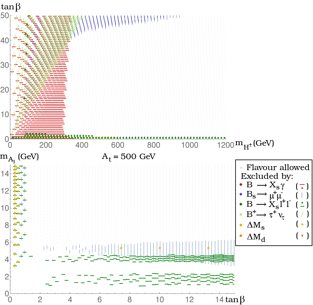
To counteract this effect, we present in Fig. 4 the limits from flavour processes obtained with the new implementation, for GeV and a somewhat heavier chargino / neutralino sector. The plot on the top again considers the plane in the MSSM limit. SUSY contributions are suppressed by the choice of low . Correspondingly, limits from only intervene in the region with low GeV. The constraints driven by eventually exclude the large range but are obviously weaker than before. On the other hand, the exclusion contour associated with and remain largely unaffected. The plot on the bottom part of Fig. 4 addresses the scenario with a light pseudoscalar: contrarily to the case of Fig. 3, CP-odd masses above GeV are left unconstrained by the flavour test, with exclusions intervening only at very-low or for in the immediate vicinity of a resonant energy (for , or ).
5.2 Impact of the new flavour tests
Beyond the observables which had been considered in [4], we have extended our analysis to several new channels. We now wish to discuss their impact on the NMSSM parameter space.

In Fig. 5, we consider the scenario of Fig. 1 once more and present the exclusion limits driven by the newly implemented channels. Note that the constraints considered in the previous section form the black exclusion zone on the background. The limits from the various channels shown in this plane seem to be essentially subleading in view of these previous constraints of Fig. 1.
- •
Limits from intervene essentially for (i.e. for constructive SUSY contributions), large (driving large SUSY contributions) and light (driving large 2HDM contributions). Yet the corresponding bounds are superseded by .
- •
intervenes in the large / low corner as well, e.g. for , but seems less sensitive than , except in the low region.
- •
The processes of the and transitions are found to be well under the current experimental upper bounds.
- •
The mixing excludes a few points (driven by where the SM is slightly off, with respect to the experimental results) but is not competitive in view of the, admittedly conservative, uncertainties.
Note that the limits induced by the channels have been omitted in Fig. 5. Given the current data, this transition would exclude the whole plane, with the exception of the large / low corner – which is excluded by most of the other flavour constraints: the significant discrepancy of the SM estimate with the experimental measurement, especially for , explains this broad exclusion range. SUSY 2HDM effects cannot reduce the gap much, except in already excluded regions of the parameter space.

Then, we return to the light pseudoscalar scenario of Fig. 3 and display the constraints associated with the new channels in Fig. 6. Again, these limits are found to be weaker than those shown in the previous section. Limits from prove the most constraining of the new channels in this regime: this again results from the enhancement of the Higgs-penguin mediated by a resonant . Subleading constraints from the mixing also intervene at low and for very light CP-odd Higgs with GeV. Again, the discrepancy among SM predictions and experimental measurements for the transition cannot be interpreted in this scenario, so that applying a CL test for the ratios would lead to the exclusion of the whole portion of parameter space displayed in Fig. 6.
Finally, we complete this discussion by considering the parameter sets of Fig. 4, where the flavour limits discussed in the previous section were found weaker. The impact of the new channels can be read in Fig. 7 The corresponding exclusion regions in the considered regime with GeV again prove narrower than those considered in Fig. 4. (Note again that we have omitted the channels, however.)

Therefore, we find that the new channels tested in bsg.f and Kphys.f are typically less constraining than the older ones, which we discussed before. Limits from and are
found to be significant, however, and an evolution of the experimental limits or an improvement in understanding the SM uncertainties may provide them with more relevance in the future. The transition stands
apart as the tension between SM and experiment resists an NMSSM interpretation, at least in the scenarios that we have been considering here.
6 Conclusions
We have considered a set of flavour observables in the NMSSM, updating and extending our former analysis in [4]. These channels have been implemented in a pair of Fortran subroutines, which allow for both the
evaluation of the observables in the NMSSM and confrontation with the current experimental results. We have taken into account the recent upgrades of the SM status of e.g. or
and included BSM effects at NLO. The tools thus designed will be / have been partially made public within the package NMSSMTools [5].
We observe that the bounds on the NMSSM parameter space driven by or have become more efficient, which should be considered in the light of the recent evolution of the SM status and/or the experimental measurement for both these channels. In particular, the large region is rapidly subject to constraints originating from the flavour sector. Similarly, the light pseudoscalar scenario is tightly corseted due to the efficiency of Higgs-penguins in the presence of such a light mediator.
Among the new channels that we have included, we note the specific status of the transition, where the discrepancy between SM and experiment seems difficult to address in a SUSY context.
Other channels of the flavour-changing sector may prove interesting to include in the future. Note e.g. the current evolution in the observables.
Acknowledgements
The author is grateful to U. Ellwanger for useful comments and thanks D. Barducci for spotting a numerical instability in the pre-released version of bsg.f.
This work is supported by CICYT (grant FPA 2013-40715-P).
References
- [1] S. Descotes-Genon, L. Hofer, J. Matias and J. Virto, arXiv:1510.04239 [hep-ph].
- [2] T. Hurth and F. Mahmoudi, Rev. Mod. Phys. 85 (2013) 795 [arXiv:1211.6453 [hep-ph]].
- [3] U. Ellwanger, C. Hugonie and A. M. Teixeira, Phys. Rept. 496 (2010) 1 [arXiv:0910.1785 [hep-ph]].
- [4] F. Domingo and U. Ellwanger, JHEP 0712 (2007) 090 [arXiv:0710.3714 [hep-ph]].
- [5]
U. Ellwanger, J. F. Gunion and C. Hugonie,
JHEP 0502 (2005) 066
[hep-ph/0406215].
U. Ellwanger and C. Hugonie, Comput. Phys. Commun. 175 (2006) 290 [hep-ph/0508022].
U. Ellwanger, J. F. Gunion, C. Hugonie, JHEP 0502 (2005) 066, arXiv:hep-ph/0406215
U. Ellwanger, C. Hugonie, Comput. Phys. Commun. 175 (2006) 290, arXiv:hep-ph/0508022http://www.th.u-psud.fr/NMHDECAY/nmssmtools.html - [6] G. Belanger, F. Boudjema, A. Pukhov and A. Semenov, Comput. Phys. Commun. 174 (2006) 577 [hep-ph/0405253].
- [7] G. Degrassi, P. Gambino and P. Slavich, Comput. Phys. Commun. 179 (2008) 759 [arXiv:0712.3265 [hep-ph]].
- [8]
F. Mahmoudi,
Comput. Phys. Commun. 178 (2008) 745
[arXiv:0710.2067 [hep-ph]].
F. Mahmoudi, Comput. Phys. Commun. 180 (2009) 1718.superiso.in2p3.fr/ - [9]
J. Rosiek, P. Chankowski, A. Dedes, S. Jager and P. Tanedo,
Comput. Phys. Commun. 181 (2010) 2180
[arXiv:1003.4260 [hep-ph]].
A. Crivellin, J. Rosiek, P. H. Chankowski, A. Dedes, S. Jaeger and P. Tanedo, Comput. Phys. Commun. 184 (2013) 1004 [arXiv:1203.5023 [hep-ph]].http://www.fuw.edu.pl/susy_flavor/ - [10]
W. Porod, F. Staub and A. Vicente,
Eur. Phys. J. C 74 (2014) 8, 2992
[arXiv:1405.1434 [hep-ph]].
http://sarah.hepforge.org/FlavorKit.html - [11] G. Buchalla, A. J. Buras and M. E. Lautenbacher, Rev. Mod. Phys. 68 (1996) 1125 [hep-ph/9512380].
- [12] K. G. Chetyrkin, M. Misiak and M. Munz, Phys. Lett. B 400 (1997) 206 [Phys. Lett. B 425 (1998) 414] [hep-ph/9612313].
- [13] M. Ciuchini, G. Degrassi, P. Gambino and G. F. Giudice, Nucl. Phys. B 527 (1998) 21 [hep-ph/9710335].
- [14] M. Ciuchini, G. Degrassi, P. Gambino and G. F. Giudice, Nucl. Phys. B 534 (1998) 3 [hep-ph/9806308].
- [15] G. Degrassi, P. Gambino and G. F. Giudice, JHEP 0012 (2000) 009 [hep-ph/0009337].
- [16] P. Gambino and M. Misiak, Nucl. Phys. B 611 (2001) 338 [hep-ph/0104034].
- [17] T. Hurth, E. Lunghi and W. Porod, Nucl. Phys. B 704 (2005) 56 [hep-ph/0312260].
- [18] A. J. Buras, P. H. Chankowski, J. Rosiek and L. Slawianowska, Nucl. Phys. B 659 (2003) 3 [hep-ph/0210145].
- [19] C. Bobeth, M. Misiak and J. Urban, Nucl. Phys. B 567 (2000) 153 [hep-ph/9904413].
- [20] C. Bobeth, A. J. Buras, F. Kruger and J. Urban, Nucl. Phys. B 630 (2002) 87 [hep-ph/0112305].
- [21] C. Bobeth, A. J. Buras and T. Ewerth, Nucl. Phys. B 713 (2005) 522 [hep-ph/0409293].
- [22] M. Misiak et al., Phys. Rev. Lett. 98 (2007) 022002 [hep-ph/0609232].
- [23] T. Becher and M. Neubert, Phys. Rev. Lett. 98 (2007) 022003 [hep-ph/0610067].
- [24] M. Misiak et al., Phys. Rev. Lett. 114 (2015) 22, 221801 [arXiv:1503.01789 [hep-ph]].
- [25] M. Czakon, P. Fiedler, T. Huber, M. Misiak, T. Schutzmeier and M. Steinhauser, JHEP 1504 (2015) 168 [arXiv:1503.01791 [hep-ph]].
- [26] C. Bobeth, M. Gorbahn, T. Hermann, M. Misiak, E. Stamou and M. Steinhauser, Phys. Rev. Lett. 112 (2014) 101801 [arXiv:1311.0903 [hep-ph]].
- [27] T. Hermann, M. Misiak and M. Steinhauser, JHEP 1312 (2013) 097 [arXiv:1311.1347 [hep-ph]].
- [28] C. Bobeth, M. Gorbahn and E. Stamou, Phys. Rev. D 89 (2014) 3, 034023 [arXiv:1311.1348 [hep-ph]].
- [29] V. Khachatryan et al. [CMS and LHCb Collaborations], Nature 522 (2015) 68 doi:10.1038/nature14474 [arXiv:1411.4413 [hep-ex]].
- [30] T. Huber, T. Hurth and E. Lunghi, JHEP 1506 (2015) 176 [arXiv:1503.04849 [hep-ph]].
- [31]
Y. Amhis et al. [Heavy Flavor Averaging Group (HFAG) Collaboration],
arXiv:1412.7515 [hep-ex].
website: www.slac.stanford.edu/xorg/hfag/ - [32] A. J. Buras, A. Czarnecki, M. Misiak and J. Urban, Nucl. Phys. B 631 (2002) 219 [hep-ph/0203135].
- [33] C. W. Bauer, Phys. Rev. D 57 (1998) 5611 [Phys. Rev. D 60 (1999) 099907] [hep-ph/9710513].
- [34] M. Benzke, S. J. Lee, M. Neubert and G. Paz, JHEP 1008 (2010) 099 [arXiv:1003.5012 [hep-ph]].
- [35] M. Czakon, U. Haisch and M. Misiak, JHEP 0703 (2007) 008 [hep-ph/0612329].
- [36] P. Gambino and U. Haisch, JHEP 0110 (2001) 020 [hep-ph/0109058].
- [37] P. del Amo Sanchez et al. [BaBar Collaboration], Phys. Rev. D 82 (2010) 051101 [arXiv:1005.4087 [hep-ex]].
- [38] A. Crivellin and L. Mercolli, Phys. Rev. D 84 (2011) 114005 [arXiv:1106.5499 [hep-ph]].
- [39] H. M. Asatrian and C. Greub, Phys. Rev. D 88 (2013) 7, 074014 [arXiv:1305.6464 [hep-ph]].
- [40] G. Hiller, Phys. Rev. D 70 (2004) 034018 [arXiv:hep-ph/0404220].
- [41]
K. A. Olive et al. [Particle Data Group Collaboration],
Chin. Phys. C 38 (2014) 090001.
website: http://pdg.lbl.gov/ - [42]
S. Aoki et al.,
Eur. Phys. J. C 74 (2014) 2890
[arXiv:1310.8555 [hep-lat]].
website: http://itpwiki.unibe.ch/flag/ - [43] P. Ball and R. Fleischer, Eur. Phys. J. C 48 (2006) 413 [hep-ph/0604249].
- [44] A. S. Cornell and N. Gaur, JHEP 0309 (2003) 030 [hep-ph/0308132].
- [45] Y. Sato et al. [Belle Collaboration], arXiv:1402.7134 [hep-ex].
- [46] W. Altmannshofer, P. Ball, A. Bharucha, A. J. Buras, D. M. Straub and M. Wick, JHEP 0901 (2009) 019 [arXiv:0811.1214 [hep-ph]].
- [47] W. Altmannshofer and D. M. Straub, Eur. Phys. J. C 73 (2013) 2646 [arXiv:1308.1501 [hep-ph]].
- [48] S. Descotes-Genon, J. Matias and J. Virto, Phys. Rev. D 88 (2013) 074002 [arXiv:1307.5683 [hep-ph]].
- [49] A. J. Buras and J. Girrbach, Rept. Prog. Phys. 77 (2014) 086201 [arXiv:1306.3775 [hep-ph]].
- [50] A. J. Buras, J. Girrbach-Noe, C. Niehoff and D. M. Straub, JHEP 1502 (2015) 184 [arXiv:1409.4557 [hep-ph]].
- [51] R. Barate et al. [ALEPH Collaboration], Eur. Phys. J. C 19 (2001) 213 [hep-ex/0010022].
- [52] J. P. Lees et al. [BaBar Collaboration], Phys. Rev. D 87 (2013) 11, 112005 [arXiv:1303.7465 [hep-ex]].
- [53] O. Lutz et al. [Belle Collaboration], Phys. Rev. D 87 (2013) 11, 111103 [arXiv:1303.3719 [hep-ex]].
- [54] A. G. Akeroyd and S. Recksiegel, J. Phys. G 29 (2003) 2311 [hep-ph/0306037].
- [55] J. F. Kamenik and F. Mescia, Phys. Rev. D 78 (2008) 014003 [arXiv:0802.3790 [hep-ph]].
- [56] S. Fajfer, J. F. Kamenik and I. Nisandzic, Phys. Rev. D 85 (2012) 094025 [arXiv:1203.2654 [hep-ph]].
- [57]
J. P. Lees et al. [BaBar Collaboration],
Phys. Rev. Lett. 109 (2012) 101802
[arXiv:1205.5442 [hep-ex]].
J. P. Lees et al. [BaBar Collaboration], Phys. Rev. D 88 (2013) 7, 072012 [arXiv:1303.0571 [hep-ex]]. - [58] J. A. Bailey et al. [MILC s Collaboration], Phys. Rev. D 92 (2015) 3, 034506 [arXiv:1503.07237 [hep-lat]].
- [59] H. Na et al. [HPQCD Collaboration], Phys. Rev. D 92 (2015) 5, 054510 [arXiv:1505.03925 [hep-lat]].
- [60] R. Aaij et al. [LHCb Collaboration], arXiv:1506.08614 [hep-ex].
- [61] M. Huschle et al. [Belle Collaboration], arXiv:1507.03233 [hep-ex].
- [62] A. Crivellin, C. Greub and A. Kokulu, Phys. Rev. D 86 (2012) 054014 [arXiv:1206.2634 [hep-ph]].
- [63] S. Bertolini, F. Borzumati, A. Masiero and G. Ridolfi, Nucl. Phys. B 353 (1991) 591.
- [64] A. J. Buras, S. Jager and J. Urban, Nucl. Phys. B 605 (2001) 600 [hep-ph/0102316].
- [65] D. Becirevic, V. Gimenez, G. Martinelli, M. Papinutto and J. Reyes, JHEP 0204 (2002) 025 [hep-lat/0110091].
- [66] A. Lenz et al., Phys. Rev. D 83 (2011) 036004 [arXiv:1008.1593 [hep-ph]].
- [67] A. Lenz and U. Nierste, arXiv:1102.4274 [hep-ph].
- [68] A. J. Buras, D. Buttazzo, J. Girrbach-Noe and R. Knegjens, arXiv:1503.02693 [hep-ph].
- [69] A. J. Buras, T. Ewerth, S. Jager and J. Rosiek, Nucl. Phys. B 714 (2005) 103 [hep-ph/0408142].
- [70] A. V. Artamonov et al. [E949 Collaboration], Phys. Rev. Lett. 101 (2008) 191802 [arXiv:0808.2459 [hep-ex]].
- [71] J. K. Ahn et al. [E391a Collaboration], Phys. Rev. D 81 (2010) 072004 [arXiv:0911.4789 [hep-ex]].
- [72] J. Bijnens, J. M. Gerard and G. Klein, Phys. Lett. B 257 (1991) 191. doi:10.1016/0370-2693(91)90880-Y
- [73] Z. Bai, N. H. Christ, T. Izubuchi, C. T. Sachrajda, A. Soni and J. Yu, Phys. Rev. Lett. 113 (2014) 112003 doi:10.1103/PhysRevLett.113.112003 [arXiv:1406.0916 [hep-lat]].
- [74] A. J. Buras and J. Girrbach, Eur. Phys. J. C 73 (2013) 9, 2560 doi:10.1140/epjc/s10052-013-2560-1 [arXiv:1304.6835 [hep-ph]].
- [75] J. A. Bailey et al. [SWME Collaboration], Phys. Rev. D 92 (2015) 3, 034510 doi:10.1103/PhysRevD.92.034510 [arXiv:1503.05388 [hep-lat]].
- [76] T. Blum et al., Phys. Rev. Lett. 108 (2012) 141601 doi:10.1103/PhysRevLett.108.141601 [arXiv:1111.1699 [hep-lat]].
- [77] N. H. Christ et al. [RBC and UKQCD Collaborations], Phys. Rev. D 88 (2013) 014508 doi:10.1103/PhysRevD.88.014508 [arXiv:1212.5931 [hep-lat]].
- [78] J. Brod and M. Gorbahn, Phys. Rev. Lett. 108 (2012) 121801 doi:10.1103/PhysRevLett.108.121801 [arXiv:1108.2036 [hep-ph]].
- [79] J. Brod and M. Gorbahn, Phys. Rev. D 82 (2010) 094026 doi:10.1103/PhysRevD.82.094026 [arXiv:1007.0684 [hep-ph]].
- [80] A. J. Buras, M. Jamin and P. H. Weisz, Nucl. Phys. B 347 (1990) 491. doi:10.1016/0550-3213(90)90373-L
- [81] Y. C. Jang et al. [SWME Collaboration], arXiv:1509.00592 [hep-lat].