Image reconstruction from dense binary pixels

The pursuit of smaller pixel sizes at ever increasing resolution in digital image sensors is mainly driven by the stringent price and form-factor requirements of sensors and optics in the cellular phone market. Recently, Eric Fossum proposed a novel concept of an image sensor with dense sub-diffraction limit one-bit pixels (jots) [1], which can be considered a digital emulation of silver halide photographic film. This idea has been recently embodied as the EPFL Gigavision camera.

We denote by $\mathrm{\bm{\mathbf{x}}}$ the radiant exposure at the camera aperture measured over a given time interval. This exposure is subsequently degraded by the optical point spread function denoted by the operator $\mathrm{\bm{\mathbf{H}}}$, producing the exposure of the sensor $\mathrm{\bm{\mathbf{\lambda}}}=\mathrm{\bm{\mathbf{Hx}}}$. The number of photoelectrons $e_{jk}$ generated at pixel $j$ in time frame $k$ follows the Poisson distribution with the rate $\lambda_{j}$. A binary pixel compares the accumulated charge against a pre-determined threshold $q_{j}$, outputting a one-bit measurement $b_{jk}$. Thus the probability of a single binary pixel $j$ to assume an ”on” value in frame $k$ is $\mathrm{P}(b_{jk}=1)=\mathrm{P}(e_{jk}\geq{q_{j}})$. Our goal is to estimate an intensity field vector $\mathrm{\bm{\mathbf{\hat{x}}}}$ best predicting $\mathrm{\bm{\mathbf{x}}}$ given the measurement matrix $\mathrm{\bm{\mathbf{B}}}$.

In [2], a maximum likelihood (ML) approach was proposed. Assuming independent measurements, the negative likelihood function can be expressed as

$$\ell(\mathrm{\bm{\mathbf{x}}};\mathrm{\bm{\mathbf{B}}})=\mathrm{const}-\sum_{kj}\log P(b_{jk}\mid q_{j},\lambda_{j}),$$

(1)

In  [2] this objective is minimized w.r.t $\mathrm{\bm{\mathbf{x}}}$ via standard iterative optimization techniques.

Since the ML approach assumes no prior, it needs a large amount of binary measurements in order to achieve good reconstruction. Sparsity priors had been shown to give state of the art results in denoising tasks in general, and particularly in low light Poisson noise [3, 4]. In this work, we show that by introducing a similar sparsity spatial prior the number of measurements can be decreased significantly. Assuming the light intensity $\mathrm{\bm{\mathbf{\lambda}}}$ admits a non-linear sparse synthesis model $\mathrm{\bm{\mathbf{\lambda}}}=\mathrm{\bm{\mathbf{H}}}\rho(\mathrm{\bm{\mathbf{Dz}}})$, with the dictionary $\mathrm{\bm{\mathbf{D}}}$ and an element-wise non-linear transformation $\rho$ such as the non-negativity enforcing function from [4], we may construct the estimator as $\mathrm{\bm{\mathbf{\hat{x}}}}=\rho(\mathrm{\bm{\mathbf{D}}}\mathrm{\bm{\mathbf{\hat{z}}}})$, where

$$\mathrm{\bm{\mathbf{\hat{z}}}}=\argmin_{\mathrm{\bm{\mathbf{z}}}}{\ell(\rho(\mathrm{\bm{\mathbf{Dz}}});\mathrm{\bm{\mathbf{B}}})+\mu\|\mathrm{\bm{\mathbf{z}}}\|_{1}}.$$

(2)

$\mu$ should be selected to best represent the tradeoff between the negative log-likelihood and the sparsity prior, in all experiments we selected $\mu$ empirically. The likelihood data fitting term is convex with a Lipschitz-continuous gradient (details are omitted due to lack of space), thus problem (2) can be solved using proximal algorithms such as FISTA [5]. Figures 2 and 3 show the significant improvement in image quality when using the sparse prior.

Iterative solutions of (2) typically require hundreds of iterations to converge. This results in prohibitive complexity and unpredictable input-dependent latency unacceptable in real-time applications. To overcome this limitation, we follow the approach advocated by [6] and [7], in which a small number of ISTA iterations are unrolled into a feed-forward neural network, that subsequently undergoes supervised training on typical inputs. In our case, a single ISTA iteration can be written in the form

$$\mathrm{\bm{\mathbf{z}}}_{t+1}\ =\sigma_{\mathrm{\bm{\mathbf{\theta}}}}\left(\mathrm{\bm{\mathbf{z}}}_{t}-\mathrm{\bm{\mathbf{W}}}\rm{diag}(\rho^{\prime}(\mathrm{\bm{\mathbf{Q}}}\mathrm{\bm{\mathbf{z}}}_{t}))\mathrm{\bm{\mathbf{H}}}^{\mathrm{T}}\nabla_{\mathrm{\bm{\mathbf{\lambda}}}}\ell(\rho(\mathrm{\bm{\mathbf{A}}}\mathrm{\bm{\mathbf{z}}}_{t});\mathrm{\bm{\mathbf{B}}})\right),$$

(3)

where $\mathrm{\bm{\mathbf{A}}}=\mathrm{\bm{\mathbf{Q}}}=\mathrm{\bm{\mathbf{D}}}$, $\mathrm{\bm{\mathbf{W}}}=\eta\mathrm{\bm{\mathbf{D}}}^{T}$, $\mathrm{\bm{\mathbf{\theta}}}=\mu\eta\mathrm{\bm{\mathbf{1}}}$ ($\eta$ is the step size used by ISTA) and $\sigma_{\mathrm{\bm{\mathbf{\theta}}}}$ is the two-sided shrinkage function. Each such operation may be viewed as a single layer of the network parametrized by $\mathrm{\bm{\mathbf{A}}},\mathrm{\bm{\mathbf{Q}}},\mathrm{\bm{\mathbf{W}}},\mathrm{\bm{\mathbf{\theta}}}$, receiving $\mathrm{\bm{\mathbf{z}}}_{t}$ as the input and producing $\mathrm{\bm{\mathbf{z}}}_{t+1}$ as the output. Figure 1 depicts the network architecture, henceforth referred to as MLNet.

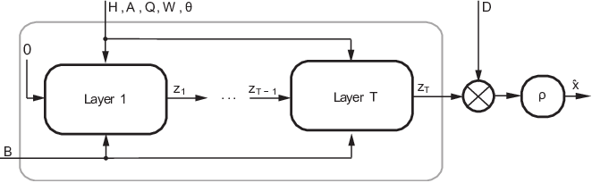
When initializing the parameters as prescribed by the ISTA iteration and then adapting them by training that minimizes the reconstruction error of the entire network, the number of layers required to achieve comparable output quality on typical inputs is smaller by about two orders of magnitude than the number of corresponding ISTA iterations (see Figure 4). To the best of our knowledge, this is the first time a similar strategy is applied to reconstruction problems with a non-Euclidean data fitting term.

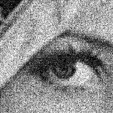
Figure 2 shows reconstruction results of an HDR image using ML with and without the sparse prior. FISTA was used to reconstruct overlapping $8\times 8$ patches that were subsequently averaged. An overcomplete dictionary was trained using $k$-SVD[8]. Figure 3 shows reconstruction results of an emulated low-light image. Figure 4 demonstrates the superiority of MLNet over iterative ML reconstruction on the same image. In all experiments $\hat{\mathrm{\bm{\mathbf{x}}}}$ was initialized to the maximum dynamic range value.

References

- [1] E. R. Fossum, “What to do with sub-diffraction-limit (sdl) pixels?–a proposal for a gigapixel digital film sensor (dfs),” in Proc. IEEE Workshop on Charge-Coupled Devices and Advanced Image Sensors, 2005, pp. 214–217.
- [2] F. Yang, Y. M. Lu, L. Sbaiz, and M. Vetterli, “Bits from Photons: Oversampled Image Acquisition Using Binary Poisson Statistics,” Tech. Rep., 2011.
- [3] R. Giryes and M. Elad, “Sparsity based poisson denoising with dictionary learning,” arXiv preprint arXiv:1309.4306, 2013.
- [4] Z. H. A. Oh and R. Willett, “To e or not to e in poisson image reconstruction.” 2014.
- [5] A. Beck and M. Teboulle, “A fast iterative shrinkage-thresholding algorithm for linear inverse problems,” SIAM Journal on Imaging Sciences, vol. 2, no. 1, pp. 183–202, 2009.
- [6] K. Gregor and Y. LeCun, “Learning fast approximations of sparse coding,” in Proc. ICML, 2010.
- [7] P. Sprechmann, A. M. Bronstein, and G. Sapiro, “Learning efficient sparse and low rank models,” arXiv preprint arXiv:1212.3631, 2012.
- [8] M. Aharon, M. Elad, and A. Bruckstein, “-svd: An algorithm for designing overcomplete dictionaries for sparse representation,” Signal Processing, IEEE Transactions on, vol. 54, no. 11, pp. 4311–4322, 2006.