Distributed robust estimation over randomly switching networks using consensusfootnoteinfo
Abstract
The paper considers a distributed robust estimation problem over a network with Markovian randomly varying topology. The objective is to deal with network variations locally, by switching observer gains at affected nodes only. We propose sufficient conditions which guarantee a suboptimal level of relative disagreement of estimates in such observer networks. When the status of the network is known globally, these sufficient conditions enable the network gains to be computed by solving certain LMIs. When the nodes are to rely on a locally available information about the network topology, additional rank constraints are used to condition the gains, given this information. The results are complemented by necessary conditions which relate properties of the interconnection graph Laplacian to the mean-square detectability of the plant through measurement and interconnection channels.
keywords
Large-scale systems, distributed robust estimation, worst-case transient consensus, vector Lyapunov functions.footnoteinfo]This work was supported by the Australian Research Council.
1 Introduction
One of the motivations for using distributed multisensor networks is to make the network resilient to loss of communication. This has led to an extensive research into distributed filtering over networks with time-varying, randomly switching topology. In particular, the Markovian approach to the analysis and synthesis of estimator networks has received a significant attention in relation to the problems involving random data loss in channels with memory which are governed by a Markov switching rule [17, 8].
In addition to capturing memory properties of physical communication channels, Markovian models allow for other random events in the network, such as sensor failures and recovery, to be considered in a systematic manner within the Markov jump systems framework. However, the Markov jump systems theory usually assumes the complete state of the underlying Markov chain to be known to every controller or filter [7] . In the context of distributed estimation and control, this requires each node of the network to know the complete instantaneous state of the network to be able to deploy suitable gains. To circumvent such an unrealistic assumption, the literature focuses on networks whose communication state is governed by a random process decomposable into independent two-state Markov processes describing the status of individual links [6, 17], even though this typically leads to design conditions whose complexity grows exponentially [6]. Also, the assumption of independence between communication links may not always be practical, e.g., when dealing with congestions.
The objective of this paper is to develop a distributed filtering technique which overcomes the need for broadcast of global communication topology and does not require Markovian segmentation of the network. Our main contribution is the methodology of robust distributed observer design which enables the node observers to be implemented in a truly distributed fashion, by utilizing only locally available information about the system’s connectivity, and without assuming the independence of communication links. This information structure constraint is a key distinction of this work, compared with the existing results, e.g., [17, 6]. In addition, the proposed methodology allows to incorporate other random events such as sensor failures and recoveries.
The paper focuses on the case where the plant to be observed, as well as sensing and communication models are not known perfectly. To deal with uncertain perturbations in the plant, sensors and communications, we employ the distributed filtering framework which has received a significant deal of attention in the recent literature [15, 18, 19]. The motivation for considering observers in this paper, instead of Kalman filters [17], is to obtain observers that have guaranteed robustness properties. It is well known that the standard Kalman filter is sensitive to modelling errors [12], and consensus Kalman filters may potentially suffer from the same shortcomings. This explains our interest in robust performance guarantees in the presence of uncertainty.
In contrast to [17, 15], in this paper the node estimators are sought to reach relative consensus about the estimate of the reference plant. As an extension of the consensus estimation methodology [9], our approach responds to the challenge posed by the presence of uncertain perturbations in the plant, measurements and interconnections. Typically, a perfect consensus between sensors-agents is not possible due to perturbations. To address this challenge, we employ the approach based on optimization of the transient relative consensus performance metric, originally proposed in [18]. We approach the robust consensus-based estimation problem from the dissipativity viewpoint, using vector storage functions and vector supply rates [4]. This allows us to establish both mean-square robust convergence and robust convergence with probability 1 of the distributed filters under consideration and guarantee a prespecified level of mean-square disagreement between node estimates in the presence of perturbations and random topology changes.
The information structure constraint, where the filters must rely on the local knowledge of the network topology, poses the main challenge in the derivation of the above-mentioned results. The standard framework of Markov jump systems is not directly applicable to the problem of designing locally constrained filters whose information about the network status is non-Markovian. To overcome this difficulty, we adopt the approach recently proposed for decentralized control of jump parameter systems [20]. It involves a two-step design procedure. First, an auxiliary distributed estimation problem is solved under simplifying assumption that the complete Markovian network topology is instantaneously available at each node. However, we seek a solution to this problem using a network of non-fragile estimators subject to uncertainty [5]. Resilience of the auxiliary estimator to uncertain perturbations is the key property to allow this auxiliary uncertain estimator network to be modified, at the second step, into an estimator network which satisfies the information structure constraint and retains robust performance of the auxiliary design.
An important question in connection with our distributed observer architecture is concerned with requirements on the communication topology under which the consensus of node observers is achievable. For networks of one- or two-dimensional agents, and networks consisting of identical agents, conditions for consensus are tightly related to properties of the graph Laplacian matrix [10, 13, 22]. In a more general situation involving nonidentical node observers, the role of the interconnection graph is often hidden behind the design conditions, e.g., see [17, 15]. Our second contribution is to show that for the distributed estimation problem under consideration to have a solution, the standard requirement for the graph Laplacian to have a simple zero eigenvalue must be complemented by detectability properties of certain matrix pairs formed by parameters of the observers and interconnections.
The paper is organized as follows. The problem formulation is given in Section 2. Section 3 studies an auxiliary distributed estimation problem without the information structure constraints. The results of this section are then used in Section 4 where the main results of the paper are given. Section 5 discusses requirements on the observer communication topology. Section 6 presents an illustrating example.
Notation
is the real Euclidean -dimensional vector space, with the norm ; ′ denotes the transpose of a matrix or a vector. Also, for a given , . , and is the identity matrix in ; we will omit the subscript when this causes no ambiguity. For , , we write (), when is positive definite (positive semidefinite). denotes the Kronecker product of matrices. is the block-diagonal matrix, whose diagonal blocks are . The symbol in position of a block-partitioned matrix denotes the transpose of the block of the matrix. is the Lebesgue space of -valued vector-functions , defined on , with the norm .
2 Problem formulation
2.1 Networks with Markovian switching topology
Consider a directed weakly connected graph , where is the set of nodes, and is the set of edges. The edge originating at node and ending at node represents the event “ transmits information to ”. In accordance with a common convention, we consider graphs without self-loops, i.e., . However, each node is assumed to have complete information about its filter, measurements and the status of incoming communication links.
We consider two types of random events at each node. Firstly, node neighborhoods change randomly as a result of random link dropouts and recovery. Also, to account for sensor adjustments in response to these changes, as well as sensor failures/recoveries, we allow for random variations of the sensing regime at each node. Letting , denote an observed process and its measurement taken at node at time , and using a standard linear relation between these quantities
| (1) |
such adjustments are associated with randomly varying coefficients , , . These random events are additional to link dropouts. This leads us to consider the combined evolution of each node’s neighbourhood and sensing regime.
Definition 1
For a node , let , be its neighbourhood set and the measurement matrix triplet, respectively, at a certain time . The pair , is said to represent the local communication and sensing state (or simply the local state) of node at time . Two states of at times , , , are distinct if , or .
From now on, we associate with every node the ordered collection of all its feasible distinct local states and denote the corresponding index . The time evolution of each local state will be represented by a random mapping .
The global configuration and sensing pattern of the network at any time can be uniquely determined from its local states. This leads us to define the global state of the network as an -tuple , where . Consider the ordered collection of all feasible global states of the network and let denote its index set. In general, not all combinations of local states correspond to feasible global states. Owing to dependencies between network links and/or sensing regimes, the number of feasible global states may be substantially smaller than the cardinality of the set of all combinations of local states. The one-to-one mapping between the set of feasible global states and its index set will be denoted , i.e., , where is the index of the -tuple . Also, we write , whenever .
Using the one-to-one mapping , define the global process to describe the evolution of the network global state. The local state processes are related to it as . Throughout the paper, we assume that is a stationary Markov random process defined in a filtered probability space , where denotes a right-continuous filtration with respect to which is adapted11 1 In the sequel, we will consider the filtration generated by a composite Markov process consisting of and error dynamics of the estimator introduced in the next section. [1]. The -algebra is the minimal -algebra which contains all measurable sets from the filtration . The transition probability rate matrix of the Markov chain will be denoted , with and [1].
Using the global state process , the time evolution of the communication graph can be represented by a random graph-valued process , whose value at every time instance is a directed subgraph of . It is assumed that for all , is weakly connected and has the same vertex set as . When , will denote the adjacency matrix of the digraph . Note that if and only if . Here and hereafter, the symbol describes the neighbourhood of node when this node is in local state . In accordance with this notation, is the neighbourhood of node when the network is in global state . Also, , , and denote the in- and out-degrees of node and the Laplacian matrix of the corresponding graph , respectively.
We will use the notation to refer to the switching network described above. Since is stationary, then each process is also stationary. However, in general the local state processes are not Markov, and the components of the multivariate process may statistically depend on each other. Hence our network model allows for dependencies between links within the network.
2.2 Distributed estimation with consensus
Consider a plant described by the equation
| (2) |
Here is the state, is a deterministic disturbance. We assume that , and that the solution of (2) exists on any finite interval , and is -integrable on .
Also, consider an observer network whose nodes take measurements of the plant (2) as follows
| (3) |
where represents the deterministic measurement uncertainty at sensing node , . The coefficients of equation (3) take values in given sets of constant matrices of compatible dimensions,
It will be assumed throughout the paper that for all and .
The measurements are processed at node according to the following estimation algorithm (cf. [17, 18, 19]):
| (4) | |||||
where is the signal received at node from node ,
| (5) |
describes the channel uncertainty affecting the information transmission from node to . It is assumed that belongs to the class of mean-square -integrable random disturbances, adapted to the filtration .
It will be further assumed that for all and , . Also in (4), , are matrix-valued functions of the local state process . These functions are the design parameters of the algorithm describing innovation and interconnection gains of the observer (4). Note that the coupling and observer gains , are required to be functions of the local state (i.e., functions of ), rather than the global state. This ‘locality’ information structure constraint is additional to the assumption about the Markov nature of the communication graph; cf. [17] where the complete communication graph was assumed to be known at each node. The problem in this paper is to determine these functions to satisfy certain robust performance criteria to be presented in Definition 2 below.
Remark 1
In equation (5), the matrices and do not depend on . This is to reflect a situation where node always broadcasts its information to node , but node randomly fails to receive this information, or chooses not to accept it, e.g. due to random congestion. It is possible to consider a more general situation where the matrices and also depend on . Technically, this more general case is no different from the one pursued here.
Associated with the system (2) and the set of filters (4) is the disagreement function (cf. [10])
| (6) |
. It represents the average (over the set of all nodes) of the total disagreement between the estimate at each node, and the estimates computed at the neighbouring nodes, when the network is in state . Following [18], we adopt to define the transient consensus performance metric in the distributed estimation problem defined below.
Let , denote the conditional probability and conditional expectation, given , . Also, given a matrix , let
Definition 2
The distributed estimation problem under consideration is to determine switching observer gains and interconnection coupling gains , for the filters (4) which ensure that the following conditions are satisfied:
- (i)
In the absence of the uncertainty, all node estimators converge exponentially in the mean-square sense and converge asymptotically with probability 1:
- (ii)
Given a constant , the following mean-square consensus performance is guaranteed
(7) - (iii)
All estimators converge in the mean-square and with probability 1:
(8) (9)
Properties (8) and (9) refer to different types of asymptotic behaviour of the estimation errors. Condition (8) states that converges to in the mean-square sense. From the Chebyshev inequality, this also implies that , that is, almost all estimator trajectories converge in sense. Property (9) states that converges to zero asymptotically for almost all realizations of the global state process . This is a stronger property; in general, it does not follow from the a.s. convergence. For that reason, both convergence properties are considered in Definition 2.
3 An auxiliary global distributed estimation problem
3.1 Non-fragile distributed estimation
In this section, we temporarily lift the locality information structure constraint and assume the global communication and sensing state process to be available at every node.
For every define , . Note that . Then, the measurements taken at node can be rewritten in terms of the global state process :
| (10) |
The auxiliary problem in this section is concerned with estimation of the state of the uncertain plant (2), (10) using a network of estimators subject to uncertainty, as follows
| (11) | |||||
Here, , are matrix-valued functions of the state of the global Markov chain to be found, and , , and are estimator perturbations. It is assumed that these perturbations are random processes adapted to the filtration and such that the multivariate process is Markov with respect to that filtration. Also in this section, it will be assumed that these uncertainties satisfy the following norm-bound conditions:
| (12) |
where , are given constants, and is the estimation error of the auxiliary estimator at node , which evolves according to the equations
| (13) | |||||
It will be shown in Section 4 that when the locality information structure constraints are imposed, this will result in an uncertainty due to the mismatch between filter error dynamics in the network subject to these constraints, and the errors which would arise in the same network if its communication state was known globally. It will be shown in the proof of Theorem 2 that this uncertainty satisfies conditions (12). The resilience of the constraint-free auxiliary network (11) to this uncertainty will be used in the next section to show that the network (4), constructed from the auxiliary solution, maintains the same convergence and robust consensus performance properties when the information structure constraints are enforced.
Definition 3
The auxiliary distributed consensus estimation problem is to determine sets of gains , , , for the filters (11) to ensure the following:
- (i)
- (ii)
- (iii)
A solution to this auxiliary problem is given in Theorem 1 below. The conditions of the theorem involve the following linear matrix inequalities in the variables , , , , , , :
| (14) | |||
where
Theorem 1
Suppose the network and the constants , , and are such that the coupled LMIs (14) and (3.1) in the variables , , , , , , , are feasible. Then the network of observers (11) with
| (22) |
solves the auxiliary estimation problem in Definition 3. The matrix in condition (7) corresponding to this solution is , where .
The proof of Theorem 1 is given in the Appendix.
3.2 Special case: Broadcast of the global state
When the global Markov state of the network is available at every node, the solution to the distributed consensus estimation problem can be obtained from Theorem 1 by letting and taking .
Corollary 1
Suppose the network and the constants and are such that the following coupled LMIs in the variables , , , , are feasible:
Then the network of observers (11) with and , defined in (22) solves the estimation problem in Definition 3. The matrix in condition (7) corresponding to this solution is , where .
4 The main result
In this section, the solution to the auxiliary distributed estimation problem developed in Section 3 will be used to obtain a distributed estimator whose nodes utilize only locally available information. This will be achieved by taking the asymptotic conditional expectation of the auxiliary gains, given a local state. Our method is based on the following technical result of [20].
Lemma 1
Suppose the Markov process is irreducible and has a unique invariant distribution . Given a matrix-valued function , for every node and for all we have:
| (28) |
Now let , , , be the coefficients of the auxiliary distributed estimator obtained in Theorem 1. Using Lemma 1, for each and we define
| (29) |
From Lemma 1, the processes are then the asymptotic minimum variance approximations of the corresponding processes . However, unlike , the evolution of is governed by the local communication and sensing state process .
To formulate the main result of this paper, consider the collection of the LMIs in the variables , , , and , consisting of the LMIs (14), (3.1), and the following additional LMIs,
where , are the same constants as those employed in the LMIs (14), (3.1), and
Also, consider the rank constraints
Theorem 2
Given a Markovian switching network and a collection of constants , , and , , associated with each node, suppose there exist matrices , , and positive scalars , , , , , which satisfy the matrix inequalities (14), (3.1), (4), and the rank constraint (4). Using the solution matrices , define the auxiliary gains
| (38) |
Next, using (29) and (38), construct the estimator network (4). The resulting distributed estimatior network solves the distributed robust estimation problem in Definition 2.
First we observe that the observer gains , constructed in this theorem, also satisfy the conditions of Theorem 1, since in view of (4). This allows us to claim that the network of auxiliary estimators (11), (38) solves the auxiliary robust estimation problem in Definition 3.
Next, consider the observer gains defined using (29) and (38). Note that for all , , and ,
Then it follows from (4) that
| (39) |
Therefore the particular perturbations in the estimators (11),
| (40) |
satisfy (12). This means that the estimator (4) in which the above particular set of gains is employed, represents one instance of the auxiliary estimator (11), corresponding to the particular perturbation (40), which is an admissible perturbation, due to (12). Therefore, since the matrices , , solve the auxiliary consensus estimation problem in Definition 3, then the distributed estimator (4) with the local gains selected above, solves the robust consensus estimation problem in Definition 2.
5 Requirements on the communication graph and interconnections
In this section, we briefly discuss necessary requirements on the network topology. Recall that condition (i) of Definition 2 requires that in the absence of perturbations, estimation error dynamics must be asymptotically stabilizable via output injection in the mean-square. This problem belongs to the class of stochastic mean-square detectability problems for linear jump parameter systems [2]. Unfortunately, even without the locality information structure constraint, there is no easy direct algebraic test to verify this property. Some conclusions can however be drawn to provide an insight into the connection between the graph Laplacian and the existence of stabilizing output injection gains.
To highlight such a connection, in this section we will make the simplifying assumption , , for all . From (38), it follows that in this case does not depend on . Hence we will also assume . Define , , , .
Let , , denote the undetectable subspace of and the unobservable subspaces of and , respectively. The following theorem shows that for the problem in Definition 2 to have a solution, every combination of undetectable states of the pairs must necessarily form an observable vector of . The proofs of this and subsequent results are removed for the sake of brevity.
Theorem 3
Suppose there exist output injection gains , , , , , such that the first condition in Definition 2(i) holds. Then,
| (41) |
We now present a necessary and sufficient condition for (41) to hold. The sufficient condition is explicitly expressed in terms of the network Laplacian matrices .
Theorem 4
One can further specialize the sufficient conditions in Theorem 4, e.g., for the cases of a balanced graph or a graph containing a spanning tree. Also, note that the information structure constraint is not used in the proofs. Therefore, the results in this section apply to more general distributed estimation problems, such as the auxiliary problem considered in Section 3.
6 Example
Consider a plant of the form (2), with , . The nominal part of the plant describes one of the regimes of the so-called Chua electronic circuit. The Chua circuit is an example of a system which switches between three regimes of operation in a chaotic fashion. For the sake of simplicity, here we consider only one regime.
The plant is observed by a 5-node switching observer network which operates intermittently in two regimes. Its graph topologies are shown in Figure 1. The evolution of the network is modelled as a two-state Markov chain with the transition probability rate matrix .

Note that the graph corresponding to state was used in [18, 21] to demonstrate synchronization of Chua systems. Indeed, the filters share the same matrix as the plant, and can be interpreted as ‘slave’ Chua systems operating in the same regime as the master. Accordingly, the convergence of the filters in our example can be interpreted as the observer-based synchronization between the slaves and the master; see [18] for further details. However different from [18], in this example the graph topology is time-varying, as explained below.
From Figure 1, nodes 3, 4, and 5 have varying neighbourhoods. Also, in this example we suppose that node 2 changes its sensor parameters when the network switches between two configurations. As a result, in this example, each local state process, except for that of node 1, has two states and always takes the same value as the global state process. On the other hand, node 1 always maintains the same local state, and its local process is constant. Therefore, we seek to obtain nonswitching observer gains for node 1 only. According to this description, in this example, , , and the mapping is as follows: , . Numerical values of the matrices , , for this example are given in Table 1; they are assumed to take one of the two values , , shown in the table. These values were chosen so that the pairs , , , corresponding to nodes 1 and 4, had undetectable modes, while node 2 was allowed to switch between detectable and undetectable coefficient pairs. Therefore, for estimation these nodes were to rely on communication with their neighbours. Also, we let , for all nodes and all , and , .
Note that both instances of the network have spanning trees with roots at nodes 3 and 5. These nodes have detectable matrix pairs , , , respectively. Also, is observable. It follows from these properties that the conditions in part (b) of Theorem 4 are satisfied. Hence, the necessary condition for global detectability, stated in Theorem 3 holds.
The design of the observer network was carried out using Matlab and the LMI solver LMIrank based on [11]. To obtain a set of non-switching gains for node 1, the norm-bounded uncertainty constraints of the form (39) were defined for the communication link at node 1, where we set , . These constants as well as were chosen by trial and error, to ensure that the corresponding rank constrained LMIs in Theorem 2 were feasible. The feasibility was achieved with . This allowed us to compute the nonswitching gains and for node 1 using (38).
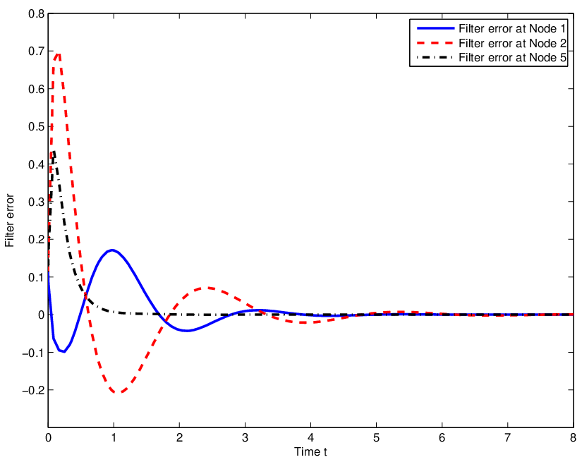
To validate the design, the system and the designed filters were simulated numerically, with a random initial condition . All uncertain perturbations were chosen to be of the form , with different coefficients and for each perturbation. Also we let , assuming an undirected nature of the channels in this example. The graphs of one realization of the global state process , and the corresponding estimation errors at nodes 1 (the nonswitching filter), 2 (the filter with the switching sensing regime) and 5 (the filter with the varying neighbourhood) are shown in Figures 2(a) and 2(b), respectively. The graph in Figure 2(b) confirms the ability of the proposed node estimators to successfully mitigate the changes in the graph topology and sensing regimes, as well as uncertain perturbations in the plant, measurements and interconnections.

7 Conclusions
The paper has presented sufficient conditions for the synthesis of robust distributed consensus estimators connected over a Markovian network. The proposed estimator provides a guaranteed suboptimal disagreement of estimates, while using only locally available information about the communication and sensing state of the network. Our conditions allow a robust filter network to be constructed by solving an LMI feasibility problem. The LMIs are partitioned in a way which opens a possibility for solving them in a decentralized manner. When the network’s global state is available at every node, this feasibility problem is convex, and the corresponding LMIs are solvable, e.g., using the decentralized gradient descent algorithm in [18]. However, the elimination of the network state broadcast has led to the introduction of rank constraints additional to the LMI conditions. Therefore, new numerical algorithms need to be developed to exploit the proposed partition of the LMIs and rank constraints. This problem is left for future research. Other possible directions for future research may be concerned with an integration of our approach with other distributed filtering techniques, such as for example, techniques involving randomly sampled measurements [16].
Acknowledgement
Discussions with C. Langbort are gratefully acknowledged.
8 Appendix: Proof of Theorem 1.
The following continuous-time counterpart of the Robbins-Siegmund convergence theorem [14] will be used in the proof of Theorem 1. Its proof is similar to [14].
Lemma 2
Consider nonnegative random processes , and adapted to a filtration , with the following properties:
- (a)
is right-continuous on ;
- (b)
is locally Lebesgue-integrable on with probability 1, i.e., almost all realizations of have the property for all ;
- (c)
;
- (d)
The following inequality holds a.s. for all
(42)
Then the limit exists and is finite with probability 1. Also, a.s..
Proof of Theorem 1
We will use the notation , , where , , . Also, , , .
Let denote the infinitesimal generator of the interconnected system consisting of subsystems (13) [1]. Consider the vector Lyapunov candidate for this system, , with quadratic components . Also, define . Since is a linear operator and for , then , where
For arbitrary , consider the expression
where we let
| (43) | |||||||
By completing the squares, one can establish that
| (44) | |||||
where
We now observe that it follows from the LMI (3.1) that for any nonzero collection of vectors
| (45) |
where are elements of the matrix , defined as
| (46) |
Together with (44), the latter inequality leads to
| (47) | |||||||
It is easy to verify using (46) that all components of the vector are negative and do not exceed , where . Hence, it follows from (43), (47) that the following dissipation inequality holds for all , , , , and for all uncertainty signals , , satisfying the constraints (12)
| (48) | |||||||
The statement of Theorem 1 now follows from (48). This can be shown using the same argument as that used to derive the statement of Theorem 1 in [18] from a similar dissipation inequality. Indeed, let , . Since equation (13) defines to be a Markov process, we obtain from (48) using the Dynkin formula that
| (49) | |||||||
Here is the expectation conditioned on the -field generated by . We now observe that the processes ,
satisfy the conditions of Lemma 2. This leads to the conclusion that a.s., and also a.s.. Due to the condition for all , we conclude that exists and a.s.. This implies with probability 1 for all and arbitrary disturbances ; i.e., (9) holds.
In the case where , , , the above observation immediately yields the statement of the theorem about internal stability of the system (13), (22) with probability 1. The claim of internal exponential mean-square stability follows directly from (48), since by definition.
Also, by taking the expectation conditioned on , on both sides of (49) and then letting , we obtain condition (7), in which . Condition (8) follows from (49) in a similar manner. Taking the expectation conditioned on , on both sides of (49), then dropping the nonnegative term and letting , we establish that . Hence .
References
- [1] A. Bain and D. Crisan. Fundamentals of Stochastic Filtering. Springer, NY, 2009.
- [2] E. F. Costa and J. B. R. do Val. On the observability and detectability of continuous-time Markov jump linear systems. SIAM J. Contr. Optim., 41:1295-1314, 2002.
- [3] L. El Ghaoui, F. Oustry, and M. Ait Rami. A cone complementarity linearization algorithm for static output-feedback and related problems. IEEE Tran. Automat. Contr., 42:1171-1176, 1997.
- [4] W. M. Haddad, V. Chellaboina, and S. G. Nersesov. Vector dissipativity theory and stability of feedback interconnections for large-scale non-linear dynamical systems. Int. J. Contr., 77:907-919, 2004.
- [5] W. M. Haddad and J. R. Corrado. Robust resilient dynamic controllers for systems with parametric uncertainty and controller gain variations. Int. J. Contr., 73:1405-1423, 2000.
- [6] C. Langbort, V. Gupta, and R. Murray. Distributed control over failing channels. Networked Embedded Sensing and Control, pp. 325–342. Springer, 2006.
- [7] L. Li, V. Ugrinovskii, and R. Orsi. Decentralized robust control of uncertain Markov jump parameter systems via output feedback. Automatica, 43:1932-1944, 2007.
- [8] I. Matei, N. C. Martins, and J. S. Baras. Consensus problems with directed Markovian communication patterns. In Proc. 2009 ACC, 2009.
- [9] R. Olfati-Saber. Distributed Kalman filtering for sensor networks. In Proc. 46th IEEE CDC, 2007.
- [10] R. Olfati-Saber and R. M. Murray. Consensus problems in networks of agents with switching topology and time-delays. IEEE Trans. Automat. Contr., 49:1520-1533, 2004.
- [11] R. Orsi, U. Helmke, and J. B. Moore. A Newton-like method for solving rank constrained linear matrix inequalities. Automatica, 42:1875-1882, 2006.
- [12] I. R. Petersen and A. V. Savkin. Robust Kalman Filtering for Signals and Systems with Large Uncertainties. Birkhäuser Boston, 1999.
- [13] W. Ren and R. W. Beard. Consensus seeking in multiagent systems under dynamically changing interaction topologies. IEEE Tran. Automat. Contr., 50:655-661, 2005.
- [14] H. Robbins and D. Siegmund. A convergence theorem for nonnegative almost supermartingales and some applications. In J. S. Rustagi, Ed., Optimizing Methods in Statistics. Academic Press, 1971.
- [15] B. Shen, Z. Wang, and Y. S. Hung. Distributed -consensus filtering in sensor networks with multiple missing measurements: The finite-horizon case. Automatica, 46:1682-1688, 2010.
- [16] B. Shen, Z. Wang, and X. Liu. A stochastic sampled-data approach to distributed filtering in sensor networks. IEEE Trans. Circuits Syst. I: Regular Papers, 58(9):2237–2246, 2011.
- [17] M. V. Subbotin and R. S. Smith. Design of distributed decentralized estimators for formations with fixed and stochastic communication topologies. Automatica, 45:2491-2501, 2009.
- [18] V. Ugrinovskii. Distributed robust filtering with consensus of estimates. Automatica, 47:1-13, 2011.
- [19] V. Ugrinovskii and C. Langbort. Distributed consensus-based estimation of uncertain systems via dissipativity theory. IET Control Theory & App., 5:1458-1469, 2010.
- [20] J. Xiong, V. A. Ugrinovskii, and I. R. Petersen. Local mode dependent decentralized stabilization of uncertain Markovian jump large-scale systems. IEEE Tran. Automat. Contr., 54:2632-2637, 2009.
- [21] J. Yao, Z.-H. Guan, and D. J. Hill. Passivity-based control and synchronization of general complex dynamical networks. Automatica, 45:2107-2113, 2009.
- [22] H. Zhang, F. L. Lewis, and A. Das. Optimal design for synchronization of cooperative systems: State feedback, observer and output feedback. IEEE Tran. Automat. Contr., 56:1948-1952, 2011.