Discrete and Continuous Systems of Logic in Nuclear Magnetic Resonance

Pedro M. Aguiar Email: pedro.aguiar@york.ac.uk Affiliation: Department of Chemistry, University of York, York YO10 5DD, UK Robert Hornby Email: robjhornby@gmail.com Affiliation: Corpus Christi College, Merton Street, Oxford OX1 4JF, UK Cameron McGarry Email: cameron@cmcgarry.co.uk Affiliation: Corpus Christi College, Merton Street, Oxford OX1 4JF, UK Simon O’Keefe Email: simon.okeefe@york.ac.uk Affiliation: Department of Computer Science, University of York, York YO10 5DD, UK Affiliation: York Centre for Complex Systems Analysis, University of York, York YO10 5DD, UK Angelika Sebald Email: angelika.sebald@york.ac.uk Affiliation: Department of Chemistry, University of York, York YO10 5DD, UK Affiliation: York Centre for Complex Systems Analysis, University of York, York YO10 5DD, UK

Abstract

We implement several non-binary logic systems using the spin dynamics of nuclear spins in nuclear magnetic resonance (NMR). The NMR system is a suitable test system because of its high degree of experimental control; findings from NMR implementations are relevant for other computational platforms exploiting particles with spin, such as electrons or photons. While we do not expect the NMR system to become a practical computational device, it is uniquely useful to explore strengths and weaknesses of unconventional computational approaches, such as non-binary logic.

keywords

Non-binary logic, ternary logic, continuous logic, nuclear magnetic resonance, spin dynamics, experimental implementation

1 Introduction

Implementations of computations on less conventional platforms such as DNA [1], slime moulds [2], oscillating chemical reactions [3] or liquid crystal media [4] have recently seen increased activities and attention with a view to exploring new ideas in the theory of logic gates. However, despite the unconventional nature of the computational platform, the form of computation in the vast majority of cases is based on a binary representation and binary logic.

The predominance of binary logic in computation is at least partly a consequence of previous choices of technology to implement computation, which worked well for binary. There are many examples of non-binary computational machines, including Babbage’s Difference and Analytic engines which used denary [5], and a wide variety of analogue systems [6]. Consideration of new, less conventional, technologies allows us to reconsider what we implement and look again at other computational systems, such as those with an unconventional base. The dynamics of nuclear spins have been explored in this context, building on previous work that looked at nuclear magnetic resonance (NMR) systems and binary logic [7].

In a computational context, the NMR system and its spin dynamics are probably more widely known for their applications in quantum computing [8]. However, nuclear spin dynamics have also played a role as an extremely versatile and highly controllable experimental platform in the implementation of classical computations [7], highlighting the advantages of the NMR system as a sandpit for design-oriented theoretical work or as a developmental tool for, for example, optical computation.

Previously we have taken an NMR-based design approach for the implementation of binary logic gates [7]. Combined consideration of theoretical descriptions of binary logic gates as well as the NMR properties of (simple) nuclear spin systems in the liquid state lead to a number of suggestions. For example, an NMR-focussed starting point suggests that a ternary logic system [9, 10] might make better use of the natural occurrence of values {-1, 0, +1} in a system made up of an ensemble of spin- $1/2$ particles than does binary logic. From the starting point of mathematical logic, it appears attractive to investigate properties of logic based on complex numbers, and how this maps to possible experimental NMR implementations.

2 Summary of NMR experiments

Before discussing ternary and complex-number based logic in the context of NMR implementations we briefly discuss some of the basic underlying principles of NMR experiments underpinning our work; we will use nomenclature introduced in earlier work [7]. Our work is restricted to some of the most simple NMR experiments.

Our samples are simple liquid compounds representing ${}^{1}\mathrm{H}$ nuclear spin systems that can be fully described by their bulk magnetisation vectors. The effects of radiofrequency (r.f.) pulses on the magnetisation vectors can be most easily visualised as (positive) rotations of the vector by a specified angle around a particular axis. This is illustrated in Figure 1(a).

Also shown are the corresponding NMR signals in the frequency domain (Fourier transformation of the observed time domain signal) carrying magnitude and phase information. Recall that observation of the bulk NMR signal is always the projection of the magnetisation vector onto the $x$ - $y$ plane. Figure 1(b) highlights the choice of signal amplitudes and phases as the basis for construction of ternary logic gates. Note that both off- and on-resonance options exist [11] for excitation as well as observation. Figure 1(a) highlights the choice of signal amplitudes and phases as the basic ingredients for construction of logic gates.

Figure 1: (a) Illustration of r.f.pulses rotating the bulk magnetisation vector away from its equilibrium

+z

orientation. (b) The magnitudes and phases of NMR signals after Fourier transformation of the time domain signals. Note that both r.f. pulses and observation can be on or off resonance [11]

3 Ternary Logic

A ternary logic function with two input variables mapping to one output value can be described by a $3\times 3$ truth table, shown in Table 1. Using the logic values of the balanced ternary system, {-1, 0, 1}, is a straightforward choice for the range of NMR experiments being considered, in which these three values occur naturally.

			B
		-1	0	1
	-1	1	0	-1
A	0	0	0	0
	1	-1	0	1

Table 1: An example of a ternary logic function - ternary multiplication, with input A on the left, input B above, and the nine output values corresponding to the nine pairs of input values in the main part of the table.

Each of the nine pairs of input values can lead to any of three output values, meaning there are $3^{9}=19{,}683$ possible functions of this sort. When attempting to implement a ternary logic function in a physical system or, inversely, trying to work out which logic functions may be implemented by a given physical system, it may be useful to classify these functions based on physical equivalences to reduce the search space; if two or more functions can be represented by an identical physical system, they need not be considered separately. These equivalences come about because any given physical implementation of a logic gate could be reinterpreted as another logic gate just by remapping the physical values of the implementation to different logic values.

For example, a binary logic gate can be represented by an electronic circuit, where a high voltage is generally chosen to correspond to a 1, but could just as easily be chosen to correspond to a 0 (with a low voltage corresponding to the other value in each case). By making use of this freedom of relabelling, more than one logic gate could be represented by the same electronic circuit.

The approach of canalising inputs taken in earlier work on binary logic [7] puts all two-input, one-output binary logic gates into four classes based on patterns in the parameters of the experiments implementing those logic gates. These four classes are the same as those produced by the Negation-Permutation-Negation (NPN) classification system[12].

In the NPN classification, two binary logic functions are considered to be in the same class if one can be converted into the other by negating input values, permuting the order of the input values, or negating the output values, in any combination. This amounts to the same thing as remapping physical values to all the possible different combinations of logic values, and so each one of these classes is a list of logic functions which can be implemented by the same physical system.

These two approaches to classifying logic gates have different ease of application in different circumstances, one being parameter-centric which is useful when looking at a physical system, and the other being based on mathematical transformations, but both lead to the classes which will aid the search for logic gate implementations. We extend the ideas of the parameter-centric canalising approach to ternary logic so that searching for implementations of ternary logic functions may be made easier.

The canalising input values approach determines which NPN classes can be implemented by a physical system by looking at how the parameters of that system behave. Specifically, it looks for values of parameters which canalise the output of the system, i.e. in a two input, one output binary logic gate, if there is a certain value for one of the inputs for which the output is a constant value, then that input value is said to be canalising. By determining the behaviour of the parameters in this way, the class of logic functions which could be mapped on to that system are found immediately.

An extension of the NPN classification of binary logic functions places the 19,683 different two-input, one-output ternary logic functions into 84 different equivalence classes[13, 14] by still allowing the order of the inputs to be swapped, and replacing the single negation function of binary logic with the six permutation functions of ternary logic. See Appendix A for details of this classification system.

The algorithms previously used for classifying a ternary logic function do not greatly simplify the search for implementations of logic gates in novel substrates because they do not obviously relate to the behaviour of parameters in physical systems. One algorithm [13], for example, takes a given logic function and transforms it into a canonical logic function which represents the class it belongs to, which does not translate to features of a physical system in a straightforward way. All of these canonical logic functions are shown in Figure 2.

Refer to caption — Figure 2: The 84 canonical logic functions with two inputs and one output which represent each of the 84 equivalence classes in this type of logic function. These functions can be transformed under the equivalences described in Appendix A to produce all 19,683 functions of this type. Each class is numbered based on the order found in previous classifications[13, 14]. The number of functions present in each class is given following the class number.

By looking at the ternary NPN classes, it is apparent that certain features which resemble the canalising inputs of binary logic functions are present within any given class, though a simple parameter-centric classification from these features has yet to be found which matches the NPN classification exactly.

A classification which contains a mixture of individual NPN classes and unions of two or more NPN classes is found when one considers a set of measures which reproduce the canalising inputs classification when applied to a binary logic gate, but can also be applied to a ternary logic gate:

•

The number of different output values in each column, with order unimportant between columns,
•

The number of different output values in each row, with order unimportant between rows.

These two measures can be taken in either order, and then every gate which has a matching set of measures is in the same parameter-centric class (PC class).

As an example, the PC class which contains the ternary multiplication function, shown in Figure 3, will have one row (or column) with a constant output value, and the other two rows (or columns) will have three different output values. In addition, one column (or row) will have a constant output value, and the other two columns (or rows) will have three different output values.

Some NPN classes share the same set of measures in the PC classification, and so some PC classes are a union of two or more NPN classes. The PC classification makes finding an implementation for a ternary logic function contained in one of the PC classes which are equal to a single NPN class more straightforward, and still narrows down the search when the ternary logic function to be implemented is in one of the PC classes with NPN overlap, although the overlap does add some of the complication back in. Adding further measures to the PC classification could separate the PC classes to be the same as the NPN classes at the cost of the simplicity of the measures.

3.1 NMR Implementations

One possible NMR implementation of a ternary logic gate can be found in an experiment with a single frequency in the spectrum, using a single pulse with flip angle, $\beta$ , and the phase, $\phi_{p}$ , as the two input parameters. This pulse sequence is shown in Figure 4(a).

A contour plot of the expected resultant magnetisation is shown in Figure 5(a). Previously, this setup has been used to implement a binary XOR gate - the chosen parameter values which represent an XOR gate are shown in the figure, and the result of performing the experiment with each combination of input values is also shown.

Figure 4: Pulse sequences used for ternary logic experiments. (a) A single square pulse of variable duration (rotation) and phase, (b) A frequency-selective pulse is followed by a delay before acquisition and (c) two square pulses each of adjustable duration (rotation) and phase. All experiments are preceded by a suitably long delay (

\tau_{\mathrm{rd}}

) to ensure the system is at equilibrium. The arched pulse in (b) is selective.

In this plot, lines have been drawn through the chosen parameter values, so that the PC measures can be found. There is a horizontal section of constant value and a vertical section of constant value, as well as two other horizontal and vertical sections which go through positive, negative and zero values. These measures define a PC class which corresponds to just one NPN class - the class which contains ternary multiplication.

If more than one NPN class corresponded to this parameter-centric classification, we would need to make further checks to confirm that ternary multiplication can be implemented, but because only one class corresponds to it, we can immediately conclude that multiplication can be implemented by this experiment, as is shown in Figure 6(b).

Another NMR implementation could make use of a sample with peaks at more than one frequency, as shown in Figure 7(a). This allows for a pulse sequence involving selective pulses and delays, see Figure 4(b). This allows two more possible parameters of the NMR experiment to be used to find logic gates with different parameter behaviours to those found in the single spectral peak experiment. The abundance of parameters and freedom to keep expanding the experiment strongly suggests that any of the 84 NPN classes of logic gates should be implementable by NMR.

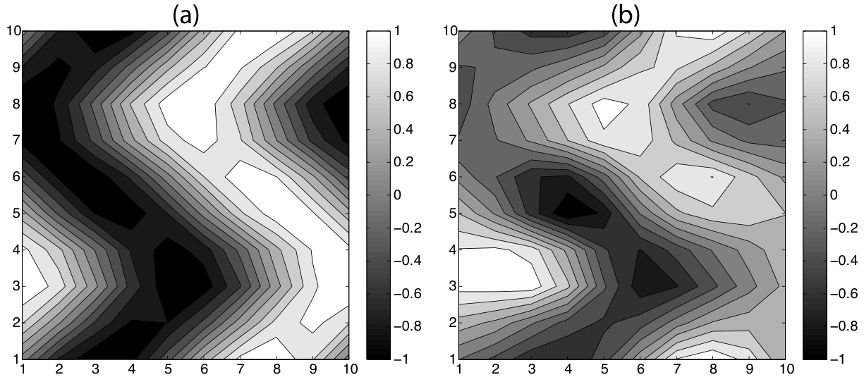
One such implementation using two spectral peaks was tested, varying the frequency of the selective pulse as one input parameter and the time delay before acquisition as the second parameter. The results of this experiment are shown in Figure 7(b), laid out as a ternary logic function table. The PC class of this experiment (and therefore the corresponding NPN classes) is one which couldn’t be achieved by the single pulse, single spectral frequency experiment.

Figure 7: (a) The sample spectrum used for the selective delay implementation, along with the transmitter frequency

\omega_{\text{rf}}

, selected so that peak B has twice the frequency difference from the transmitter as peak A, so that the spins of B will have precessed twice as far as the spins of A in a time delay before acquisition,

\tau_{d}

. (b) The result of using the pulse sequence in Figure 4(b) with the selected values for

\tau_{d}

and

\omega_{p}

shown.

\tau_{1}

corresponds to an acquisition delay which allows the spins of B to precess by

\pi

(the spins of A precess by

\pi/2

), and

\tau_{1}

allows the spins of A to precess by

\pi

(the spins of B precess by

2\pi

). The selective frequency of the pulse,

\omega_{p}

, leads to a signal from either A, B, or neither. The integral of the resulting frequency domain signal corresponds to the logic values shown.

To begin exploring beyond ternary logic, an experiment involving two pulses was performed on a sample with a single spectral peak. The pulse sequence for this experiment is shown in Figure 4(c).

Two of the pulse parameters were varied sequentially: the flip angle, $\beta_{1}$ , of pulse one, and the phase, $\phi_{p2}$ of pulse two. The other parameters were set to fixed values, $\phi_{p1}=\frac{\pi}{2}$ and $\beta_{2}=\frac{\pi}{2}$ . 100 results were taken, in a 10x10 grid with values of $\beta_{1}$ taken evenly spaced over the interval $[0,2\pi]$ and $\phi_{p2}$ also evenly sampled over $[0,2\pi]$ .

These data were compared to a theoretical model and were shown to match the expected results to within a small error, showing that the system of predicting NMR experimental outcomes is robust. The comparison of the theoretical results and the measured results is shown in Figure 8. This array of values leads to the idea of continuous logic.

4 Continuous Complex-Number-Based Logic

Rather than using the discrete truth-values found in Boolean algebra, it has been established that a system of continuous logic can be implemented that uses continuous truth-values to express uncertainty [15]. In an attempt to extend upon the ideas of the previous section we construct Complex Logic, a system of logic that has been split into two parts based on the exponential form of complex numbers: Magnitude Logic (mLogic) and Phase Logic (pLogic).

When representing information as a complex number, we can arbitraily define any function on $n$ complex numbers in terms of two other functions

f(z_{1},\cdots z_{n})=g(r_{1},\cdots r_{n})\exp(ih(\theta_{1},\cdots\theta_{n}))

(1)

where $z_{k}=r_{k}e^{i\theta_{k}}$ . The following subsections focus on the ways in which these functions can be defined in order to produce a meaningful logic. The possible choices for $g$ are described by mLogic and those for $h$ by pLogic. A more mathematically rigorous approach to continuous logic can be found in appendix B.

4.1 Magnitude Logic

Fuzzy logic is a form of continuous logic that has been well-developed elsewhere [15]. Here we state that all aspects of mLogic corresponds in some way to fuzzy logic. For this to be the case it is necessary that only complex numbers with magnitude $r\in[0,1]$ are considered.

When refering to the comparison between mLogic and pLogic with fuzzy logic, the operations in Fuzzy Logic will be refered to as “normal fuzzy logic operators” and denoted mathematically by a subscript $0$ . mLogic and pLogic operators are denoted by a subscript $m$ and $p$ respectively.

For any mLogic operator acting on a complex number, the result will have the same phase but with a magnitude defined by the normal fuzzy logic operator. For some operator $F_{m}$ , the fuzzy logic match is $F_{0}$ such that

F_{m}(re^{i\theta})=F_{0}(r)e^{i\theta}.

(2)

One example is the unary operator NOT where $\neg_{0}x=1-x$ , it follows then that

\neg_{m}(re^{i\theta})=(1-r)e^{i\theta}.

(3)

More generally, for an operation that is not necessarily unary

F_{m}(z_{,}\cdots z_{n})=F_{0}(r_{1},\cdots r_{n})e^{i\theta_{\mathrm{res}}}

(4)

where $z_{k}=r_{k}e^{i\theta_{k}}$ and $\theta_{\mathrm{res}}=\theta_{\mathrm{res}}(\theta_{1},\cdots\theta_{n})$ can be defined arbitrarily. The ways in which $\theta_{\mathrm{res}}$ can be defined are discussed in section 4.3.

For example AND ( $\wedge$ ) with $x\wedge_{0}y=xy$ gives

z_{1}\wedge_{m}z_{2}=r_{1}r_{2}e^{i\theta_{\mathrm{res}}}

(5)

where $\theta_{\mathrm{res}}=\theta_{\mathrm{res}}(\theta_{1},\theta_{2})$ must be defined separately as in equation 1.

The representation of a magnitude in the NMR system is achieved by taking advantage of the $T_{1}$ decay [11] as illustrated in Figure 9. We begin from equilibrium magnetisation (that is, $\mathbf{M}$ aligned along the $+z$ direction, parallel to the external magnetic field) and apply a $\pi$ pulse after which $\mathbf{M}$ will be aligned along $-z$ . $\mathbf{M}$ immediately begins to decay back towards the equilibrium position over time $t$ according to

\mathbf{M}(t)=M(0)\left[1-2e^{-t/T_{1}}\right]\mathbf{\hat{z}}.

(6)

We are free to choose the delay $t=\tau_{\mathrm{dec}}$ such that the magnitude $r$ is described by the ratio $\alpha M(t)/M(0)$ . The constant $\alpha$ can be chosen arbitraily in order to present a range of magnitudes $r\in[0,\alpha]$ . In the case of mLogic $\alpha=1$ . Depending on how much time one allows for this relaxation process, different magnitudes of the magnetisation vector can be read out at different times.

A $(-\frac{\pi}{2})_{y}$ pulse is then applied so that $\mathbf{M}$ lies along the positive $x$ -axis. The intensity of the output signal is used to calulate the magnitude. The pulse sequence and corresponding movement of the vector are described in Figure 9. Such an experiment is more commonly used to determine the value of $T_{1}$ [11].

Figure 9: A pulse sequence capable of encoding magnitude along with a schematic of the evolution of the net magnetisation

\mathbf{M}

throughout the sequence at the points (i) through (iv). Filled pulses represent rotations of the magnetisation by

\pi

and unfilled by

\frac{\pi}{2}

4.2 Phase Logic

When dealing with the phase of a complex number, we must take into account that generally $e^{i\theta}=e^{i(\theta+2\pi n)}$ . For this reason it is defined that all phases shall be expressed with $\theta\in[0,2\pi)$ and all arithmetic of phases is modulo $2\pi$ .

In pLogic, it is defined that $0$ represents truth and $\pi$ falsehood. There are then two domains in which no member has absolute truth or absolute falsehood: $\Theta_{1}=(0,\pi)$ and $\Theta_{2}=(\pi,2\pi)$ . There is a relation between the truth values in pLogic and those in fuzzy logic: for any truth value defined in pLogic (a pTruth value) $\theta$ , there is an equivalent truth value in fuzzy logic given by the projection function.

T_{0}(\theta)=\frac{\lvert\pi-\theta\rvert}{\pi}.

(7)

It is obvious that for each $\theta_{1}\in\Theta_{1}$ there exists $\theta_{2}\in\Theta_{2}$ such that $T_{0}(\theta_{1})=T_{0}(\theta_{2})$ and that $\theta^{\prime}=2\pi-\theta$ . Equivalently the phase-truth of some complex number $z$ is identical to that of its complex conjugate $z^{*}$ as illustrated in Figure 10.

Figure 10: Comparision of pTruth values of complex numbers on the unit circle. Note the pTruth of

z=e^{i\phi}

is the same as that of its complex conjugate with a similar relationship for

-z

and

-z^{*}

. Note also the two domains,

\Theta_{1}

marked by the upper (thick, solid) arc and

\Theta_{2}

marked by the lower (thick, dashed) arc.

The representation of phase in the NMR system is implemented in a way that could be combined with the magnitude implementation described above. Again, starting from equilibrium, a $(-\frac{\pi}{2})_{y}$ pulse is applied so that $\mathbf{M}$ is aligned along the positive $x$ -axis. Now the vector is viewed in a rotating frame offset from the on-resonance frame by a frequency $\frac{\omega_{\mathrm{off}}}{2\pi}$ .

In this frame the vector is allowed to precess for a time $\tau_{\mathrm{rd}}$ , such that for a desired phase $\theta$

\omega_{\mathrm{off}}\tau_{\mathrm{d}}=\theta.

(8)

The encoded phase is computed from the Fourier transform of the measured time domain signal. The pulse sequence is shown in Figure 11(a). We also encode the phase in the on-resonance frame, using a pulse sequence described in Figure 11(b). The former method was found to be broadly more reliable.

Figure 11: Pulse sequences used for complex logic experiments. The experiments in (a) and (b) are both used to encode phase while that of (c) can encode magnitude and phase. The presence of multiple pulses in (b) and (c) require repetition with phase cycling as shown below sequence to compensate for instrumental imperfections. Grey pulses are of variable duration, unfilled pulses correspond to

\frac{\pi}{2}

pulses and black to

\pi

rotations.

As with mLogic, it is defined that a pLogic operation (denoted $F_{p}$ ) acting on some complex number is related to the fuzzy logic equivalent. However, it is not a simple case of writing $F_{p}(re^{i\theta})=r\exp(iF_{0}(\theta))$ since the fuzzy operations do not reflect the new truth-values (as defined above).

We define an operation in fuzzy logic $F$ to match a function in pLogic $F_{\mathrm{peq}}$ under the condition that

T_{0}(F_{\mathrm{peq}}(\theta_{1},\cdots\theta_{n}))=F_{0}(T_{0}(\theta_{1}),\cdots T_{0}(\theta_{n})).

(9)

An operation from fuzzy logic can then be described in pLogic by

F_{p}(re^{i\theta})=r\exp(iF_{\mathrm{peq}}(\theta)).

(10)

Mirroring the behaviour of mLogic, the phase operations alone do not define the magnitude of the output in a non-unary operation. For example, pXNOR

r_{1}e^{i\theta_{1}}\overline{\oplus}_{p}r_{2}e^{i\theta_{2}}=r_{\mathrm{res}}e^{i(\theta_{1}+\theta_{2})},

(11)

where $r_{\mathrm{res}}=r_{\mathrm{res}}(\theta_{1},\theta_{2})$ is not defined as in equations 1 and 5.

4.3 Combined Complex-Number-Based Logic

It just so happens that when complex number multiplication is substituted for $f$ in equation 1, ( $f(z_{1},z_{2})=z_{1}\times z_{2}$ ), the resulting expression gives an mAND and a pXNOR gate

$\displaystyle g(r_{1},r_{2})$	$\displaystyle=r_{1}\times r_{2}=r_{1}\wedge r_{2}$	(12)
$\displaystyle h(\theta_{1},\theta_{2})$	$\displaystyle=\theta_{1}+\theta_{2}\mod 2\pi=\theta_{1}\overline{\oplus}\theta_{2}$	(13)
$\displaystyle z_{1}\times z_{2}$	$\displaystyle=\underbrace{r_{1}r_{2}}_{\text{mAND}}\exp({i(\underbrace{\theta_{1}+\theta_{2})}_{\text{pXNOR}}}).$	(14)

We thus have the operations necessary for a half adder [16].

This is just one example of many possible Complex Logic Gates that combine magnitude and phase logic.

In order to implement such a gate it is necessary to combine the magnitude and phase implementation as described above. In this process, $\mathbf{M}$ is manipulated to encode magnitude exactly as before but an additional precession time is allowed before the measurement. In this way the magnetisation vector in the $x$ - $y$ plane has both magnitude and phase encoded in it. The process is depicted in Figure 11(c).

This process is used to implement complex number multiplication: by choosing $\tau_{dec}$ and $\tau_{d}$ appropriately it was possible to position $\mathbf{M}$ in the x-y plane at any position. Arbitrary scaling of the maximum length of $\mathbf{M}$ allows any magnitude to be chosen.

Such experiments are highly accurate, with the magnitude accurate to five parts in one thousand and the phase to one part in one hundred. This is demonstrated in Figure 12.

5 Experimental

5.1 Spectrometer

All $\mathrm{{}^{1}H}$ NMR experiments were performed on a Bruker Avance II 700 NMR spectrometer (corresponding to a $\mathrm{{}^{1}H}$ Larmor frequency $\frac{\omega_{0}}{2\pi}=$-700.13\text{\,}\mathrm{MHz}$$ ) equipped with a commercial triple-resonance ( $\mathrm{{}^{1}H}$ / $\mathrm{{}^{13}C}$ / $\mathrm{{}^{15}N}$ ) probe at $T=$289\text{\,}\mathrm{K}$$ . Samples were contained in standard $5\text{\,}\mathrm{mm}$ o.d. NMR tubes. Durations of (calibrated) non-selective $\frac{\pi}{2}$ pulses were of the order of $7.5\text{\,}\mathrm{\SIUnitSymbolMicro s}$ .

5.2 Samples and Experiments

$\mathrm{{}^{1}H}$ NMR experiments on ternary logic were carried out on a sample of $99.9$ percent deuterated $\text{CDCl}{\vphantom{\text{X}}}_{\smash[t]{\text{3}}}$ to which a small amount of $\text{H}{\vphantom{\text{X}}}_{\smash[t]{\text{2}}}\text{O}$ was added. This sample provided two well separated $\mathrm{{}^{1}H}$ resonances originating from $\text{H}{\vphantom{\text{X}}}_{\smash[t]{\text{2}}}\text{O}$ and residual $\text{CHCl}{\vphantom{\text{X}}}_{\smash[t]{\text{3}}}$ (see Figure 7). Relaxation delays of $5\text{\,}\mathrm{s}$ were found to be sufficient. Selective excitation experiments were performed using Gaussian excitation profile pulses of duration $4.244\text{\,}\mathrm{ms}$ corresponding to a $\frac{\pi}{2}$ rotation.

All $\mathrm{{}^{1}H}$ NMR experiments on complex number based logic were carried out on the $\mathrm{{}^{1}H}$ NMR resonance of residual $\text{CHCl}{\vphantom{\text{X}}}_{\smash[t]{\text{3}}}$ in a sample of $99.9$ percent deuterated $\text{CHCl}{\vphantom{\text{X}}}_{\smash[t]{\text{3}}}$ . The sample was contained in an NMR tube fitted with a J. Young valve. The $\mathrm{{}^{1}H}$ $T_{1}$ value for the sample was determined to be $7.6\pm\pm 0.1\text{\,}\mathrm{s}$ , using standard inversion recovery[11]. Applying standard phase cycling, precision of phase and magnitude outputs were found to be one part in one thousand and one part in ten thousand respectively.

(a)

(b)

Figure 12: Complex number multiplications using the phase sequence in Figure 11(c). and show the mean measured result vs the anticipated for magnitude and phase respectively.

Simulations of the NMR experiments used to implement ternary logic gates were created using Matlab R2012b (8.0.0.783).

6 Outlook

In the light of our experimental implementations it should be abundantly clear that we do not advertise NMR-based computation as a particularly practical approach. However, nuclear spin dynamics are eminently rich and controllable and, thus, ideally suited as a design tool and sandpit for all kinds of exploration and scrutiny when developing new ideas in logic gates and circuitry. This is particularly true in that a wide variety of implementations can be tested on the same system and will allow for direct comparisons of concepts of cost, robustness, or error-propagation behaviour.

As far as NMR systems are concerned we have so far barely scratched the surface of the richness of its parameter space: we have solely considered nuclear spin dynamics in small molecules at ambient conditions, in a strong and homogeneous external magnetic field in the presence of rapid isotropic molecular tumbling and in the absence of internuclear dipolar coupling interactions. This narrow window provides particularly straightforward experimental conditions as the underlying nuclear spin dynamics can be fully described by a vector picture [11].

If more complicated nuclear spin dynamics “hardware” is required, it will be extremely straightforward to exploit more of the capabilities of NMR systems. For example, using an additional magnetic field gradient across the volume of a single-component sample will encode a range of Larmor frequencies over the sample volume, similar to the techniques used for spatial encoding in medical applications of magnetic resonance [11]. Such manipulations may have attractive features regarding parallel operations or in the creation of dynamic memory.

One could alternatively use chemical samples of a more complicated make-up, with multiple different sites and isotopes (and corresponding resonance frequencies). Potentially this could include internuclear dipolar couplings and could be combined with more sophisticated techniques, such as those found in two-dimensional NMR experiments [11].

While there may be rather obvious potential benefits from increasingly complicated nuclear spin dynamics, the drawback is that for many such systems one will have to employ numerical simulations to predict and engineer the exact behaviour of the NMR system. In itself this is not a problem but it has some impact on the role of NMR systems as a sandpit for developmental work for unconventional computations that could subsequently be implemented on other physical systems. While numerically exact simulations are perfectly feasible for even quite complicated nuclear spin systems and NMR experiments [11], this option does not normally exist to the same degree for other physical systems.

This is particularly relevant when seeing the (spin based) NMR system as a development and checking tool for other spin-based methods, say optical computation. Optical computation is far more likely to eventually become a practical computational approach and may benefit from developmental work using NMR systems — as long as there is no need for numerical simulations.

Finally we mention in passing that one of the features that renders NMR computation less practical is the timescales of operation: even under favourable conditions such as we used here in solution-state NMR, relaxation times for nuclear spin ensembles to return to equilibrium magnetisation (equivalent to a refreshed system) are of the order of several to many tens of seconds (and can be much longer in other forms of condensed matter). However, the natural slowness of the system, together with the timescales of r.f. pulses of the order of $\mu\mathrm{s}$ , allows for the design of unusual systems in which many computational steps are reversible to a very good degree of approximation.

7 Acknowledgements

We gratefully acknowledge support of our work by the York Centre for Complex Systems Analysis (YCCSA) summer schools 2014 and 2015.

Appendix A Ternary Classes

Two ternary logic functions which take two inputs and give one output, $f_{1}(x,y)$ and $f_{2}(x,y)$ , are considered to be in the same Negation-Permutation-Negation (NPN) class if they are equivalent under any of three definitions:

Equivalence A: $f_{1}(x,y)$ is equivalent to $f_{2}(x,y)$ if $f_{1}=P_{i}(f_{2})$ for any of the permutation functions, $P_{i}$ , of the set $(0,1,2)$ . That is, permuting the output of one function leads to another function in the same class.

Equivalence B: The two functions are equivalent if $f_{1}(x,y)=f_{2}(P_{i}(x),P_{j}(y))$ . That is, permuting the input values of a function leads to a function in the same class.

Equivalence C: The two functions are equivalent if $f_{1}(x,y)=f_{2}(y,x)$ . That is, swapping the order of the inputs gives another function in the same class.

These equivalences are illustrated in Figure 3.

Appendix B Generalised Continuous Logic

pLogic as defined in section 4 is only one possible reinterpretation of continuous logic and may not be suitable for implementation in other systems.

Define a Continuous Logic of order $n$ as a 4-tuple

L=(\Lambda,I,B,\preceq).

(15)

•

$\Lambda$ is the Logical Domain, an interval.
•

$I\subset\Lambda$ is a tuple of the $n$ absolutes with $I=(\iota_{0},\iota_{1},\cdots\iota_{n-2},\iota_{n-1}).$ These are generalisations of the concepts of “True” and “False.”
•

$B$ is the set of base gates, the distinct functions that will act on members of $\Lambda$ .
•

Implicitly defined is $G$ , the set of all possible gates $G$ where for any $g\in G$ , $g$ is some partial composition of any number of members of $B$ .
•

$\preceq$ is a transitive, reflexive, antisymmetric, binary function that partially orders $G$ , with the additional requirement that for all $k,k+1\in I$ and all $\iota_{j}\in I$ we have $\iota_{k}\preceq\iota_{k+1}$

The properties of any base gate $b\in B$ of order $m$ are as follows

1.

$b:\Lambda^{m}\rightarrow\Lambda$
2.

it is not possible to construct the function $b$ from some partial composition of other members of $B$ .

For example, conventional fuzzy logic is described by

L_{\mathrm{Fuzzy}}=([0,1],(0,1),B_{\mathrm{Fuzzy}},\leq)

(16)

for an appropriate choice of $B_{\mathrm{Fuzzy}}$ such as XNOR and fanout.

A logic is said to be gate-complete under the condition that $G$ is a set of all possible functions that can act on the domain. Equivalently, that $B$ forms a set of universal gates.

Now consider any two logics $L=(\Lambda,I,B,\preceq)$ and $L^{\prime}=(\Lambda^{\prime},I^{\prime},B^{\prime},\preceq^{\prime})$ with corresponding $G$ and $G^{\prime}$ respectively. We now state that all $\lambda\in\Lambda$ , $\iota\in I$ , $g\in G$ and equivalently for the primed logic $\lambda^{\prime}\in\Lambda^{\prime}$ , etc.

We say that $L$ projects to $L^{\prime}$ under a surjective function $T:\Lambda\rightarrow\Lambda^{\prime}$ if for all $\iota_{k}$ and $\iota_{k}^{\prime}$ we have

T(\iota_{k})=\iota_{k}^{\prime}

(17)

$T$ is known as the projecting function and any $\lambda$ and $\lambda^{\prime}$ with $T(\lambda)=\lambda^{\prime}$ are called equivalent truth values.

For any such logics, a function $g$ can be said to weakly match a function $g^{\prime}$ under the condition that

T(g(\iota_{1},\cdots\iota_{m}))=g^{\prime}(T(\iota_{1}),\cdots T(\iota_{m}))

(18)

which is denoted

g\sim_{T}g^{\prime}

(19)

Furthermore, a function $g$ can be said to strongly match some $g^{\prime}$ if

T(g(\lambda_{1},\cdots\lambda_{m}))=g^{\prime}(T(\lambda_{1}),\cdots T(\lambda_{m}))

(20)

which is denoted

g\simeq_{T}g^{\prime}

(21)

For any $L$ and $L^{\prime}$ , $L$ weakly corresponds to $L^{\prime}$ under $T$ if

1.

$L$ projects to $L^{\prime}$ under $T$
2.

For each $g$ there exists some $g^{\prime}$ such that $g\sim_{T}g^{\prime}$

in which case we write

L\approx_{T}L^{\prime}.

(22)

$L$ strongly corresponds to $L^{\prime}$ under $T$ if

1.

$L$ projects to $L^{\prime}$ under $T$
2.

For each $g$ there exists some $g^{\prime}$ such that $g\simeq_{T}g^{\prime}$

in which case we write

L\approxeq_{T}L^{\prime}.

(23)

It can then be shown that pLogic weakly corresponds to Fuzzy Logic under projecting function $T_{0}$ as given in equation 7 and the sets of functions contain only the NOT, XOR and XNOR gates. It might be possible to define further gates that will match in the two systems but that is not discussed here.

A final point is on the intervals of the logical domains that are between any two absolutes, which we shall call absolute intervals. In pLogic, there are two such domains, $\Theta_{1}=(0,\pi)$ and $\Theta_{2}=(\pi,2\pi)$ as depicted in figure 10. This maps exactly to binary continuous logic, since each truth value corresponds to one in the interval $(0,1)$ .

However, if pLogic is modified so that, for example, $I=\{0,\frac{2\pi}{3},\frac{4\pi}{3}\}$ we will have a continuous ternary logic (as opposed to the discrete ternary logic described in Section 3. There are now three absolute intervals: $(0,\frac{2\pi}{3})$ , $(\frac{2\pi}{3},\frac{4\pi}{3})$ and $(\frac{4\pi}{3},0)$ . Such a system is depicted in Figure 13.

Figure 13: A variation on phase logic containing three absolutes and hence three absolute intervals,

\Theta_{0}

\Theta_{1}

and

\Theta_{2}

which are marked by solid, dashed and thick lines respectively.

One might think that this could trivially map to some corresponding modification of binary continuous logic with $I=\{0,\frac{1}{2},1\}$ but that is not the case as there are now only two absolute intervals: $(0,\frac{1}{2})$ and $(\frac{1}{2},1)$ . It would therefore be impossible to describe a truth-value that is somewhere between $1$ and $0$ whereas this can be done in the modified pLogic.

We suggest that by a suitable generalisation of the work here it may be possible to describe any $n^{\mathrm{th}}$ order logic with absolute domains for any two absolutes in the Logic.

References

[1] M. Amos, G. Paun, G. Rozenberg, and A. Salomaa. (2002). Topics in the theory of DNA computing. Theoretical Computer Science, 287(1):3 – 38. Natural Computing.
[2] J. G. Whiting, B. P. de Lacy Costello, and A. Adamatzky. (2014). Slime mould logic gates based on frequency changes of electrical potential oscillation. Biosystems, 124:21–25.
[3] J. Gorecki, K. Gizynski, J. Guzowski, J. Gorecka, P. Garstecki, G. Gruenert, and P. Dittrich. (2015). Chemical computing with reaction–diffusion processes. Phil. Trans. R. Soc. A, 373(2046):20140219.
[4] S. Harding and J. F. Miller. (2005). Evolution in materio: Evolving logic gates in liquid crystal. In In Proceedings of the workshop on unconventional computing at ECAL 2005 VIIIth European, page 12.
[5] D. Swade. (2002). The Difference Engine: Charles Babbage and the Quest to Build the First Computer. Penguin Books.
[6] K. Murrell, D. Holroyd, National Museum of Computing, and National Museum of Computing Staff. (2013). The Harwell Dekatron Computer. National Museum of Computing.
[7] M. Bechmann, A. Sebald, and S. Stepney. (2012). Boolean logic gate design principles in unconventional computers: an nmr case study. International Journal of Unconventional Computing, 8(2):139–159.
[8] J. A. Jones. (2011). Quantum-computing with NMR. Progress in Nuclear Magnetic Resonance Spectroscopy, 59:91–120.
[9] M. Glusker, D. Hogan, and P. Vass. (July 2005). The ternary calculating machine of Thomas Fowler. Annals of the History of Computing, IEEE, 27(3):4–22.
[10] N. P. Brusentsov and J. R. Alvarez. (2011). Ternary computers: The setun and the setun 70. In J. Impagliazzo and E. Proydakov, editors, Perspectives on Soviet and Russian Computing, volume 357 of IFIP Advances in Information and Communication Technology, pages 74–80. Springer Berlin Heidelberg.
[11] M. H. Levitt. (2008). Spin Dynamics: Basics of nuclear magnetic resonance, 2 edition. John Wiley & Sons, Ltd. Chichester.
[12] V. P. Correia and A. Reis. (2001). Classifying n-input boolean functions. In in Proc. IWS, page 58.
[13] A. Lloris and J. Velasco. (July 1981). Classification under permutations of the ternary functions of two variables. Computers and Digital Techniques, IEE Proceedings E, 128(4):143–148.
[14] T. Soma and T. Soma. (May 2011). Classification of ternary logic functions by self-dual equivalence classes. In Multiple-Valued Logic (ISMVL), 2011 41st IEEE International Symposium on, pages 33–37.
[15] V. Levin. (2000). Continuous logic i. basic concepts. KYBERNETES, 29(9-10):1234–1249.
[16] A. S. Tanenbaum and J. R. Goodman. (1998). Structured Computer Organization, 4th edition. Prentice Hall PTR, Upper Saddle River, NJ, USA.