CacheDiff: Fast Random Sampling

In this paper, we study the following problem:

This problem has been studied extensively in [6, 4, 2, 5, 7, 1]. The applications of this problem span from security to big data. However, the approaches in [6, 4, 2] have time complexity of $O(N)$, which is not very efficient to use to sample in big data when $N$ is often very big or to generate random codes whose probability to be guessed is extremely small. In [7], Vitter presented an acceptance-rejection method to sequentially select $k$ items from a pool of given $N$ items uniformly with complexity of approximately $O(k)$ when $k$ is very small compared to $N$. The experiments in [7] shows that when $\text{$k$}\geq 0.15\text{$N$}$, the running time of the acceptance-rejection method is worse than the reservoir sampling in [6]. In particular, the acceptance-rejection method only works with known $N$.

Random sampling algorithms are useful in several areas:

• •

  Big data: Instead of processing all data items, we can process only process a subset of the items to obtain approximate results. The subset of the items can be selected by randomly sample $k$ items from all the data items.

• •

  Election polling: To estimate the approximation approval rate of election candidates, instead of conducting a full survey, we can randomly select people to obtain their opinions on candidates.

• •

  Online tickets: Each user when buying an online ticket will be generated a code that is very difficult to predict by hackers. To avoid the code duplication for different tickets, the codes are generated in batches by selecting randomly $k$ integers (each selected integer is a code) from the integers between 0 and $N$. To make the codes very difficult to predict, then $k$ need to be very small compared to $N$.

It is rather straightforward to see that Problem 1 can be solved using a random permutation (shuffling) algorithm.

Algorithm 1 above requires time and space complexity of $O(N)$, which can be prohibitive in big data or highly secure random code generators. However, note that Problem 1 is equivalent to the following problem:

Algorithm 2 solves Problem 2. Not that Algorithm 2 is similar to Algorithm 1. Algorithm 2 still requires $O(N)$ time and space. However, note that when $k$ is very small compared to $N$, $\text{$k$}\ll\text{$N$}$, $\text{$index$}[\text{$i$}]=\text{$i$}$ for most of $i$. Because the array of integers from 0 to ($N$-1) can be stored very efficiently, as a result, to store the $index$ array, we only need to cache the value in the $index$ array that $\text{$index$}[\text{$i$}]\neq\text{$i$}$. We can implement this caching using a hash table. As a result, we can improve the time and space complexity of Algorithm 2 using Algorithm 3.

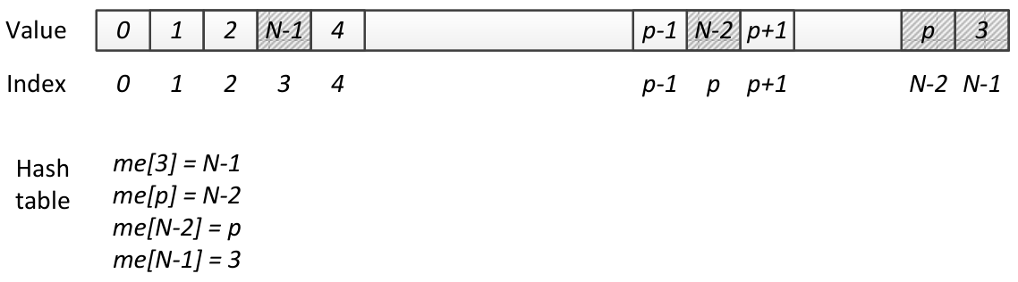
Algorithm 3 improves from Algorithm 2 in both time and space complexity by using a hash table to store the difference between the output array and the simple array of integers from 0 to $N$-1. Because we only select $k$ items, as a result, the space complexity of the hash table $me$ is $O(\text{$k$})$. Then it is easy to see that Algorithm 3 runs in average time complexity of $O(\text{$k$})$ and requires $O(\text{$k$})$ space.

Figure 1 illustrates the CacheDiff technique. In the first iteration, 3 is selected so we swap 3 and $N$-1. The entries at 3 and $N$-1 now become different from the indices so the hash table caches the values at those entries. Similarly for the second iteration when $p$ is selected.

Proof: First, we prove that the probability that an index is not selected after $n$ iterations of the for loop at line 3 is $\frac{\text{$N$}-\text{$n$}}{\text{$N$}}$. We will prove it using induction. For $\text{$n$}=1$, then $\text{$i$}=\text{$N$}-1$, as a result, the probability that the index is selected is $\frac{1}{\text{$N$}}$. Suppose that our hypothesis holds for $\text{$n$}=\text{$m$}$, we will prove that it holds for $\text{$n$}=\text{$m$}+1$. At iteration $\text{$n$}=\text{$m$}+1$, $\text{$i$}=\text{$N$}-\text{$m$}-1$. Then the probability that the index is selected due to the random selection at line 3 is $\frac{1}{\text{$N$}-\text{$m$}}$. Then the probability that the index is not selected at iteration $\text{$n$}=\text{$m$}+1$ is $1-\frac{1}{\text{$N$}-\text{$m$}}=\frac{\text{$N$}-(\text{$m$}+1)}{\text{$N$}-\text{$m$}}$. As a result, the probability that the index is not selected after $\text{$n$}=\text{$m$}+1$ iterations is $\frac{\text{$N$}-\text{$m$}}{\text{$N$}}\times\frac{\text{$N$}-(\text{$m$}+1)}{\text{$N$}-\text{$m$}}=\frac{\text{$N$}-(\text{$m$}+1)}{\text{$N$}}$, which is what we want to prove.

So after $k$ iterations, the probability that one index is not selected is $\frac{\text{$N$}-\text{$k$}}{\text{$N$}}$, then the probability that the index is selected in one of the $k$ iteration is $1-\frac{\text{$N$}-\text{$k$}}{\text{$N$}}=\frac{\text{$k$}}{\text{$N$}}$.$\hfill\Box$

In this paper, we demonstrated the use of a hash table to store a small number of modified entries within a predictable sequence, in the words of information theory [3], the sequence has a small entropy. This method lead to a simple algorithm that has lower complexity than [6, 4, 2, 5, 1] or easier to understand and implement than [7].

References

- [1] J. H. Ahrens and U. Dieter. Sequential random sampling. ACM Trans. Math. Softw., 11(2):157–169, June 1985.
- [2] M. T. Chao. A general purpose unequal probability sampling plan. Biometrika, 69(3):pp. 653–656, 1982.
- [3] Thomas M. Cover and Joy A. Thomas. Elements of Information Theory (Wiley Series in Telecommunications and Signal Processing). Wiley-Interscience, 2006.
- [4] Pavlos S. Efraimidis and Paul G. Spirakis. Weighted random sampling with a reservoir. Inf. Process. Lett., 97(5):181–185, March 2006.
- [5] Xiangrui Meng. Scalable simple random sampling and stratified sampling. In Sanjoy Dasgupta and David Mcallester, editors, Proceedings of the 30th International Conference on Machine Learning (ICML-13), volume 28, pages 531–539. JMLR Workshop and Conference Proceedings, May 2013.
- [6] Jeffrey S. Vitter. Random sampling with a reservoir. ACM Transactions on Mathematical Software (TOMS), 11(1):37–57, March 1985.
- [7] Jeffrey Scott Vitter. Faster methods for random sampling. Commun. ACM, 27(7):703–718, July 1984.