A coupled D Babcock–Leighton solar dynamo model.
I. Surface magnetic flux evolution
Abstract
The need for reliable predictions of the solar activity cycle motivates the development of dynamo models incorporating a representation of surface processes sufficiently detailed to allow assimilation of magnetographic data. In this series of papers we present one such dynamo model, and document its behavior and properties. This first paper focuses on one of the model’s key components, namely surface magnetic flux evolution. Using a genetic algorithm, we obtain best-fit parameters of the transport model by least-squares minimization of the differences between the associated synthetic synoptic magnetogram and real magnetographic data for activity cycle 21. Our fitting procedure also returns Monte Carlo-like error estimates. We show that the range of acceptable surface meridional flow profiles is in good agreement with Doppler measurements, even though the latter are not used in the fitting process. Using a synthetic database of bipolar magnetic region (BMR) emergences reproducing the statistical properties of observed emergences, we also ascertain the sensitivity of global cycle properties, such as the strength of the dipole moment and timing of polarity reversal, to distinct realizations of BMR emergence, and on this basis argue that this stochasticity represents a primary source of uncertainty for predicting solar cycle characteristics.
Subject headings
dynamo — Sun: activity — Sun: magnetic fields — Sun: photosphere — sunspotsI. Introduction
The Sun’s magnetic field is generated by a magnetohydrodynamical induction process, or a combination of processes, taking place primarily in the solar convection zone. On small spatial scales, convection is believed to continuously process and replenish the photospheric magnetic field, through a local dynamo mechanism that is statistically stationary and does not produce net signed flux. At the other extreme, magnetic fields developing on spatial scales commensurate with the solar radius show a strong degree of axisymmetry and a well-defined dipole moment, and undergo polarity reversals on a regular cadence of approximately eleven years (see review by Hathaway 21).
Cowling’s theorem dictates that such an axisymmetric large-scale magnetic field cannot be sustained by purely axisymmetric flows. Convective turbulence represents an ideal energy reservoir for the required dynamo action, provided the Coriolis force can break the mirror symmetry that would otherwise prevail. This process can be quantified using mean-field electrodynamics, leading to the so-called -effect, an electromotive force proportional to the mean magnetic fields (for a recent review see, e.g., Charbonneau 11). That such a turbulent dynamo, acting in conjunction with differential rotation, can lead to the production of large-scale magnetic fields undergoing polarity reversals has been confirmed by both laboratory experiments [29, 14, 55] and global magnetohydrodynamical (MHD) numerical simulations of solar convection (see Charbonneau 11, § 3.2, and references therein).
The Coriolis force also acts on the flows developing along the axis of buoyantly rising toroidal magnetic flux ropes, believed to be generated near the base of the solar convection zone, and eventually piercing the photosphere in the form of bipolar magnetic regions (hereafter BMRs; see Fan 19 for a review). This rotational influence produces the observed systematic east–west tilt characterizing large BMRs, as embodied in Joy’s Law. Associated with this tilt is a net dipole moment so that, effectively, a poloidal magnetic component is being produced from a pre-existing toroidal component. Here again it is the Coriolis force that ultimately breaks the axisymmetry of the initially purely toroidal flux rope, so the process is akin to a large-scale version of the -effect. With shearing by differential rotation producing a toroidal magnetic component from a pre-existing poloidal component, the dynamo loop can be closed. This forms the basis of the Babcock–Leighton dynamo models [1, 31], which have undergone a strong revival in the past two decades and are now considered a leading explanatory framework for the solar magnetic cycle (for a recent review, see, e.g., Karak et al. 25).
In such models, the transport and accumulation in polar regions of the magnetic flux liberated at low latitudes by the decay of a BMR is what sets the magnitude of the resulting dipole moment and the timing of its reversal [50, 52]. The cross-equatorial diffusive annihilation of magnetic flux associated with the leading members of tilted BMRs is ultimately what allows the build-up of a net hemispheric signed flux (see Cameron et al. 6, Cameron et al. 8, and references therein). Indeed, only a small fraction of emerging magnetic flux eventually makes it to the poles; the magnetic flux in the polar cap at sunspot minimum, , is about the same as the unsigned flux in a single, large BMR, and the net axial dipole moment of all BMRs emerging during a typical cycle is a few times the dipole moment required for polarity inversion [51]. Consequently, one large BMR emerging very close to the equator with a significant tilt can have a strong impact on the magnitude of the dipole moment building up in the descending phase of the cycle, and thus on the amplitude of the subsequent cycle (see, e.g., Jiang et al. 23).
In this series of papers we present a novel Babcock–Leighton model of the solar cycle based on the coupling of a surface flux transport (SFT) simulation with a mean-field-like interior dynamo model. We henceforth refer to this hybrid as a “D model”, as it couples a two-dimensional simulation on a spherical surface () to a two-dimensional simulation on a meridional plane (), each simulation providing the source term required by the other.
In the present paper we focus on the SFT component of the model. SFT has been extensively studied in the past decades, starting with the work of Leighton [30] up to recent attempts to reproduce the details of modern magnetograms (see reviews by Sheeley 40, Mackay & Yeates 32, and Jiang et al. 24). The model’s behavior relative to emergence and model characteristics are fairly well understood (see, e.g., Baumann et al. 3). In particular, observed magnetographic features, such as poleward flux strips (“surges”), require a delicate balance between meridional circulation and the surface effective diffusion rate (see, e.g. Wang et al. 49), ultimately driven by the dispersive random walk taking place at the supergranular scale. Yet, due to limitations in the measurement of these two processes, their detailed parameterization remains, even today, a matter of debate, with the consequence that SFT models continue to differ significantly in their outputs. This is an unsatisfactory situation, considering how useful accurate and spatially resolved representations of surface magnetic flux evolution would be for data assimilation-based cycle prediction schemes (e.g., Kitiashvili & Kosovichev 26, Dikpati et al. 16, and references therein). Moreover, the availability of realistic, detailed surface magnetic maps associated with distinct dynamo regimes is needed in reconstructing the heliospheric magnetic field in the distant past (see, e.g., Riley et al. 36). In order to build a SFT model that behaves, as much as possible, like the Sun —one to be ultimately used as the key surface component of a solar-like Babcock–Leighton dynamo model— calibration against observations needs to be performed thoroughly. Some quantitative studies have been conducted (see, e.g., Yeates 54), but never through systematic optimization procedures. This is what we aim to achieve in the present study.
We first discuss the formulation of the SFT model itself (§ 2), after which we turn to its calibration against observed data. Toward this end we used a genetic algorithm, which allows an efficient exploration of the model’s parameter space, as well as the identification of parameter correlations and degeneracies (§ 3). We then repeat the analysis while allowing the meridional flow to vary systematically in the course of the cycle, as suggested by observations. In § 4 we explore the model behavior with respect to the stochastic variability inherent to emergence statistics. We conclude by comparing and contrasting our optimized SFT model to similar models available in the extant literature. Coupling to the dynamo simulation, and the resulting solar cycle model, is the subject of the following paper in this series (A. Lemerle & P. Charbonneau 2015, in preparation).
II. Model
As new BMRs emerge at the surface of the Sun and subsequently decay, their magnetic flux is dispersed and transported with the plasma by surface flows, and locally destroyed or amplified according to basic rules of electromagnetic induction. For physical conditions representative of the solar photosphere, this process is well described by the MHD induction equation:
| (1) |
with the net magnetic diffusivity, including contributions from the small microscopic magnetic diffusivity (with the electrical resistivity of the plasma), as well as a dominant turbulent contribution associated with the destructive folding of magnetic field lines by small-scale convective fluid motions. A dynamically consistent approach would require Equation (1) to be augmented by the hydrodynamical fluid equations including Lorentz force and Ohmic heating terms. However, on spatial scales commensurate with the solar radius, the use of a kinematic approximation, whereby the flow u is considered given, has been shown to be quite appropriate in reproducing the synoptic evolution of the solar surface magnetic field [48, 3, see, e.g.,]. We adopt this kinematic approach in what follows, and solve Equation (1) on a spherical shell representing the solar photosphere.
On spatial scales much larger than convection, only meridional circulation and differential rotation contribute to u in Equation (1). Both these flows can be considered axisymmetric () and steady () to a good first approximation. Since we solve the induction equation on the solar surface, meridional circulation reduces to a latitudinal flow .
Following earlier modeling work on surface magnetic flux evolution, we consider the magnetic field to be predominantly radial on global scales and we solve only the -component of Equation (1), after enforcing the null divergence condition throughout:
| (2) |
where is the uniform surface diffusivity. Note the addition of two supplementary terms: a source term , with the Dirac delta, to account for the emergence of new BMRs at given positions and times , to be extracted from some suitable observational database (see § III.1), and a linear sink term to allow for some exponential decay of the surface field with time. This term thus mimics the radial diffusion and mechanical subduction of locally inclined magnetic field lines, which cannot be captured by Equation (2) and the assumption of a purely radial surface magnetic field. The addition of this sink term is also motivated by the analysis of Schrijver et al. [38], who found that such decay on a timescale of was necessary to preclude secular drift and ensure polarity reversal of the polar caps when modeling surface flux evolution over many successive cycles. Baumann et al. [2] argued that this exponential destruction of surface magnetic flux could be justified physically as the effect of a vertical turbulent diffusion (including convective submergence) on the decay of the dominant dipole mode. In what follows we treat as a free parameter. Equation (2) is now a two-dimensional linear advection–diffusion equation for the scalar component at the surface of the Sun, augmented by source and sink terms.
II.1. Meridional circulation
Because the solar meridional surface flow is weak and thus difficult to measure accurately (but do see Ulrich 45), its latitudinal dependence has been approximated by a number of ad hoc analytical formulae: some as minimalistic as a , with peak at latitude [17, e.g.], some displacing the peak flow to lower latitudes by introducing exponents to the and terms [47, 53, e.g.], others using a truncated series expansion [37], or shutting down the flow speed to zero near the poles [46, e.g.], for a closer fit to the observed motion of surface magnetic features [27, 20, 42].
The recent observational determinations of Ulrich [45], however, suggest the existence of a more complex latitudinal pattern, increasing quite rapidly from the equator to a peak amplitude near to latitude, and decreasing more slowly to zero up to – latitude. To account for such asymmetric rise and fall of the flow speed at low–mid latitudes and possible suppression of the flow at high latitudes, we opt to use the following, versatile analytical formula:
| (3) |
with the maximum flow velocity and , , , and free parameters to be determined in the course of the foregoing analysis. With the same in both hemispheres, the profile is antisymmetric with respect to the equator. It takes approximately the shape of a profile in the case , , , and , with peak at mid–latitudes. Varying parameters and allows the latitude of peak flow speed to be moved to either lower latitudes () or higher latitudes (). High values for both and broaden the peak between low and high latitudes. Values of have the effect of stopping the flow before the poles, at lower latitudes as increases. Growing values of have the same effect near the equator, but since such a low-latitude plateau seems far from a solar behavior, we set for the remainder of our analysis. The top panel of Figure 1 illustrates a few sample profiles. Note in particular that, with appropriate choices for , and , Equation (3) can reproduce most profiles in use in the literature (see bottom panel).
Analyses by Ulrich [45] also show latitudinal flow speeds dropping to negative values near the poles, especially at the beginning and end of cycles. Since this pattern is at the limit of observational determinations and does not appear in all cycles or solar hemispheres, we opt not to model these potential high-latitude secondary flow cells. We also use the same value of in both hemispheres.
II.2. Differential rotation
Unlike meridional circulation, the surface differential rotation profile is observationally well established. We adopt here the parametric formulae calibrated helioseismically by Charbonneau et al. [12]:
| (4) |
with and . The angular velocity is lowest at the poles and highest at the equator, where (see also Snodgrass 41).
II.3. Magnetic diffusivity
Near the solar surface, the magnetic diffusivity due to Ohmic dissipation reaches . However, as initially shown by Leighton [30], surface convective motions at the supergranular scale drive a random walk that disperses magnetic flux, and can be modeled as a diffusive process characterized by an effective magnetic diffusivity of order . The exact value is virtually impossible to determine from first principles, so we henceforth treat as a free parameter to be determined by our analysis.
II.4. Numerical solution
The adimensional form of the surface transport Equation (2) is solved numerically in a two-dimensional Galerkin finite-element scheme (see, e.g., Burnett 5), over a regular Cartesian grid in with longitudinal periodicity, the latter enforced through a padding of ghost cells, updated at every time step. The zero-flux polar boundary condition is hardwired at the level of the finite-element scheme itself. Because only a small fraction of emerging magnetic flux ends up accumulating at the poles, it is essential to rigorously ensure magnetic flux conservation. Consequently, the numerical discretization errors must be monitored and kept in check.
Using double precision arithmetic, a longitude–latitude grid is required to ensure that net signed surface flux never exceeds of the total unsigned surface flux, at least an order of magnitude better than observations (see, e.g., Figure 2e). With such a grid, relatively short time steps are also necessary to ensure stability, which is of the order of time steps per year, for a total of time steps per solar cycle.
II.5. Numerical optimization
The final formulation of Equation (2) leaves us with a set of six unknown parameters (, , , , , and ), which we aim to constrain quantitatively based on magnetographic observations of the solar surface.
We opt to compare a time–latitude map of longitudinally averaged output from our model with an equivalent longitudinally averaged magnetogram. For this purpose, Hathaway [21] has provided us with his well-known ‘‘magnetic butterfly diagram’’ data11 1 http://solarscience.msfc.nasa.gov/images/magbfly.jpg, made available from 1976 August to 2012 August, at a temporal resolution of one point per Carrington rotation and data points equidistant in . The data are a compilation of measurements from instruments on Kitt Peak and SOHO, corrected to obtain the radial component of the magnetic field.
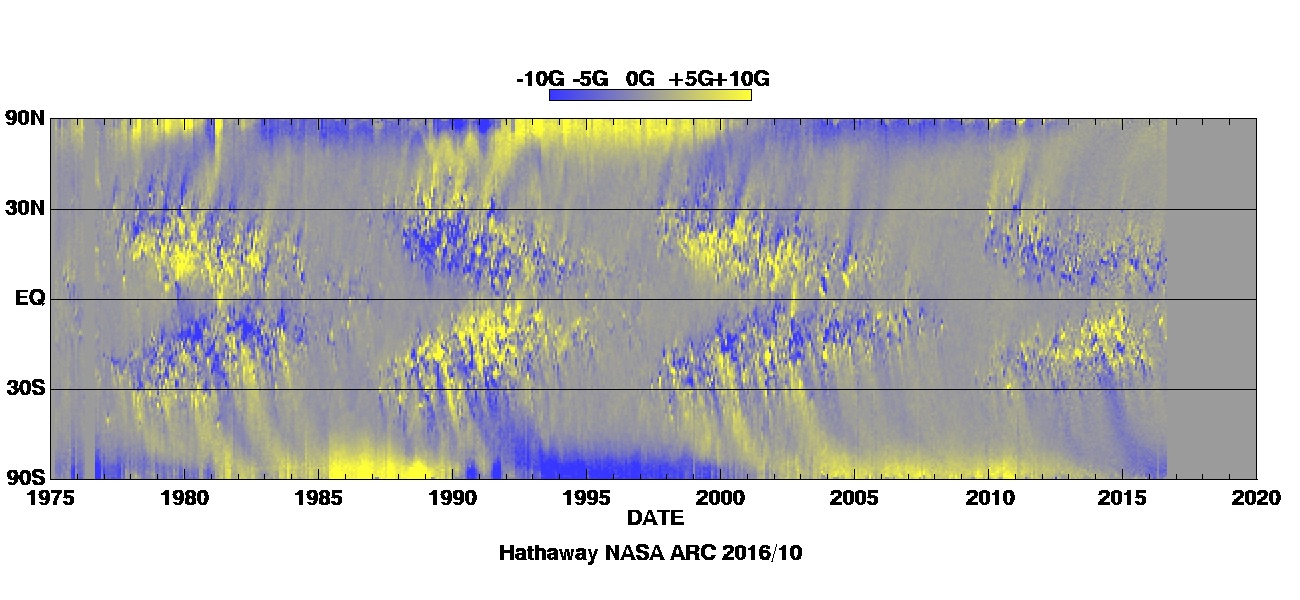
As a unique optimization criterion for the model, a plain minimization of the residuals between the two maps represents the most straightforward approach. Unfortunately, this turns out to be insufficient to properly constrain the model parameters, for a number of reasons including high-latitude artifacts, as well as observational size and magnetic field thresholds leading to missing flux. Therefore, in addition to fitting the time–latitude synoptic map, we add further constraints by putting more weight on two physically meaningful features: first, the evolution of the overall axial dipole moment (divided by ), defined as
| (5) |
and, second, the shape of mid–latitudes flux-migration strips. To quantify the latter, we delimit two “transport regions”, one in each hemisphere (regions T1 and T2 in Figure 2a, latitudes to ), dominated by inclined flux strips and where very little flux emerges or accumulates. We then calculate the latitudinal average of in each region, a quantity directly influenced by the amount of flux and the width and inclination of flux strips:
| (6) |
With such definitions, both of the above surface integrals end up having the same physical unit, with magnitude of the order of a few Gauss.
Constraining the behavior of the axial dipole component, and indirectly the times of polarity reversals, should help constrain the values of diffusivity and exponential decay time , which directly shape the polar magnetic caps, as well as meridional circulation parameters (, , , and ), which dictate how new flux migrates toward the poles and eventually triggers the polarity reversals. The extent of polar caps down to latitude also suggests a significant decrease of the meridional flow near these high latitudes. Similarly, diffusivity will shape the width and length of mid–latitudes flux-migration strips, and the meridional circulation profile will set their inclination in the synoptic map.
To obtain a final optimization criterion, we evaluate the rms deviation between simulated map and measured map, the rms deviation between simulated and measured , and the rms deviations between simulated and measured . We combine them as follows, such that the overall rms deviation must be minimized:
| (7) |
This multi-objective optimization criterion goes significantly beyond the cross-correlation approach introduced by Yeates [54], since it defines an absolute least-squares minimization of the differences between the model and observations, rather than being restricted to their temporal synchronisation.
The inverse of the quantity is defined as our merit function, or ‘‘fitness’’. We seek to maximize this fitness using the genetic algorithm-based optimizer PIKAIA 1.2, a public domain software distributed by HAO/NCAR22 2 http://www.hao.ucar.edu/modeling/pikaia/pikaia.php (2015 March). Genetic algorithms (GA) are a biologically inspired class of evolutionary algorithms that can be used to carry out global numerical optimization. PIKAIA [13, 10] is one such classical GA-based optimizer. PIKAIA evolves an optimal solution to a given optimization task by selecting the better solutions among a population of trial solutions, and breeding new solutions through genetically inspired operations of crossover and mutation acting on a string encoding of the selected solution’s defining parameters. In this manner GA allow efficient, adaptive exploration of parameter space through parallel processing of advantageous substrings. Indeed, GA-based optimizers have proven quite robust in handling global optimization problems characterized by complex, multimodal parameter spaces that often trap gradient-based optimizers in local extrema. For an accessible introduction to GA and their use for numerical optimization, see Charbonneau [9].
In the present context PIKAIA is operating in a seven-dimensional parameter space (see Table 1), with the fitness measure given by Equation (7). We use the default settings for PIKAIA’s internal control parameters, with the exception of encoding depth, population size, mutation mode (equiprobable digitcreep, with fitness-based adjustment), and number of generational iterations.
As numerical optimization algorithms, GA tend to be computationally expensive, as the number of model evaluations is equal to the population size times the number of generational iterations. In most model fitting tasks reported upon in what follows, a population size of 48 trial solutions evolving over 500 generations was found to be sufficient to reliably ensure proper convergence of all model parameters. This adds up to 24000 model fitness evaluations per optimization run. Calculating the fitness of a single trial solution (seven-parameter vector) implies running a SFT simulation, calculating the various integrals introduced in § II.5, and finally evaluating Equation (7). For our working spatial mesh and time step this requires a little under 10 minutes on a single-core modern CPU, adding up to core-days for a typical optimization run. However, this sequence of operations is applied independently to each member of the population, and so can easily be carried out in parallel (see, e.g., Metcalfe & Charbonneau 34). With the only information returned by each evaluation being the fitness, near-perfect parallelization can be achieved, by assigning one core per population member, thus bringing the wall-clock time down to a few days.
One specific feature of PIKAIA deserves further discussion, namely its adaptive mutation rate. Throughout the evolution, PIKAIA monitors the fitness differential and spread of the population in parameter space, and whenever these quantities become too small (large), the internal mutation rate is increased (decreased), while ensuring that the current best individual is always copied intact into the next generation. This effectively leads to a form of Monte Carlo exploration of parameter space in the vicinity of the current optimum, allowing escape from local extrema as the case may be. At the same time, this pseudo-random sampling of parameter space taking place about the current optimum solution can be harnessed to construct error estimates on solution parameters; these estimate remain useful even though, strictly speaking, population members are not statistically independent of one another since they have all been bred from the same earlier generations.

III. Solar cycle 21: a case study
III.1. Surface emergence database
In an effort to characterize the details of surface flux evolution during sunspot cycle 21, Wang & Sheeley [51] (hereafter WS) have assembled a comprehensive database of over 3000 observed BMRs, each approximated as a pair of poles of identical magnetic flux but opposite polarity. Their input data consisted of daily magnetograms recorded at the National Solar Observatory/Kitt Peak between 1976 August and 1986 April. For each BMR, they list the time, magnetic flux, polarity of the western pole, and latitude and longitude of each pole, measured when their magnetic flux reached its peak. Positive magnetic fluxes range from to , for a total of for the whole database. As described in WS’s analysis, while the latitude and time of emergence of the BMRs follow the usual butterfly pattern, the polarities of western poles are predominantly coherent in a given hemisphere and opposite in the other hemisphere, as per Hale’s law. The database also shows a slight hemispheric asymmetry of in favor of the northern hemisphere, in both total flux and number of BMRs.
We use WS’s updated database entries as direct inputs for the SFT source term . Each th BMR is injected in the surface layer at its observed time , colatitude , and longitude , with a gaussian distribution for each pole:
| (8) |
where and are the heliocentric angular distances from the centres and of the two poles, respectively, and the width of the gaussian. We set this width to a fixed value for all emergences, in order to minimize numerical errors, a choice that may induce only slight shifts in the times of emergences. In other words, our Gaussian-shape BMRs are injected with a larger area than observed, but this does not impact the subsequent evolution since Gaussian profiles spread in a shape-preserving manner under the sole action of diffusion. Also, the use of heliocentric distances ensures that the surface integral of can be calculated exactly as the measured flux, provided that magnetic field amplitude at the centre of the gaussian is adjusted accordingly. This appropriate geometry also guarantees that total signed flux from both poles cancels completely. This condition is important since any remnant net surface flux was found to accumulate during the simulation. All these factors considered, along with a tight grid and double precision arithmetic, the net magnetic flux from one discretized BMR rarely exceeds times the emerged flux in the positive pole.
III.2. Initial condition
As we aim to reproduce, among other global cycle features, the timing of polar cap polarity reversals, the amount and distribution of magnetic flux at the beginning of the cycle is particularly crucial. Even if we assumed an axisymmetric initial condition, the synoptic data compiled by Hathaway [21] remain incomplete for this 1976-1977 activity minimum. In fact, while the southern hemisphere presents the expected quantity of negative flux, the northern hemisphere presents no clear polar cap, and even some substantial negative flux through the end of 1976 (see Figure 2a). Figure 2e illustrates how the corresponding signed magnetic flux is far from zero for this period, even reaching the value of unsigned flux at one point. Figure 3a illustrates the latitudinal distribution of in 1976 June, patently not mirror-symmetric about the equatorial plane.
In order to construct a plausible initial condition, we turn to observed distributions for other cycle minima. Figure 3b illustrates latitudinal distributions of at the beginnings of cycles 22–24, normalized to unity in each hemisphere. Apart from the unusually asymmetric profile for cycle 21, the latitudinal distributions are characterized by a low field strength from the equator to latitude, followed by a rise to maximum field strength near latitude, in both hemispheres. The amplitude appears to fall near the poles for some activity minima, but we do not take this feature into account considering the lower reliability of high-latitude line-of-sight magnetographic measurements. While the simple axisymmetric profile
| (9a) | |||
| has been adopted by many authors [43, 50, e.g.], a curve of the form | |||
| (9b) | |||
fits better the measurements shown in Figure 3. We test both functional forms in what follows. In both cases, the same amplitude is used in the two hemispheres, to ensure a zero net flux, but is kept as a seventh free parameter to be optimized along with the six physical parameters described above.
Finally, for the same reason that prevents us from using 1976 June measurements as an initial condition, we should probably not expect to reproduce the synoptic magnetogram for early cycle 21. We therefore choose to perform our optimization over the period going from 1977 June to 1986 Septembre.
III.3. Reference case
As a benchmark for subsequent comparison, we first look at the behavior of our model using some typical parameter values found in the literature. Baumann et al. [3] presented a detailed study of the effect of varying parameters on a SFT model similar to ours. For their reference case, they used a diffusivity and a maximum meridional flow velocity , with the profile by van Ballegooijen et al. [46], as illustrated in Figure 1. This profile can be closely approximated by our adopted profile (Equation (3)), by setting , , and . They did not use any exponential decay term, which is similar to adopting in Equation (2). Figure 2b illustrates the results of our SFT simulation in such a parameter regime (listed in the first column of Table 1), starting with the initial condition by Svalgaard et al. [43].
Visual comparison of panels (a) and (b) of Figure 2 is encouraging, with some typical mid–latitude flux-migration strips of the right polarity, and accumulation of polar flux at about the right time and amplitude. However, the rms deviation between this time–latitude map and its observed counterpart (Figure 2a) is , which is quite high. Moreover, an excessive quantity of opposite magnetic flux accumulates in polar regions during the second half of the cycle, with final unsigned magnetic flux reaching about twice the observed value of at the end of the cycle (cf. black and red dashed curves in Figure 2e). The comparison worsens further when looking at the evolution of the axial dipole moment (Figure 2f): the simulated curve diverges markedly from observations, with . Again, the initial axial dipole is too strong, but this does not prevent an early reversal and the building of dipolar moment in excess of the observed value by over a factor of two. This excessive transport of flux toward the poles is presumably due to a combination of a slow poleward flow at low latitudes, allowing too much of the polarity of the BMRs’ western poles to cancel at the equator, and a fast latitudinal transport of the remaining polarity at mid/high latitudes. This suggests the use of a suboptimal meridional circulation profile.
The detailed shape of flux-migration strips, evaluated using the integrated magnetic field in the transport regions T1 (Figure 2g) and T2 (Figure 2h), does not compare well to observations either ( and ). The subdued variability reveals a temporal widening of the flux strips, likely due to an excessive surface magnetic diffusivity. Altogether, these features lead to a combined rms difference between this reference case and observations ().
| Symbol | Reference | Tested | Optimal |
|---|---|---|---|
| Value | Interval | Solution | |
| () | () | ||
| G | |||
| aa is similar to removing the term in Equation (2). | years | ||
| \reciprocal | |||
| \reciprocal |
III.4. Optimal solution
We perform our main optimization of the cycle 21 simulation and its seven-parameters set (hereafter W21-7), based on fitness (Equation (7)). For each parameter, we choose an interval to be explored that is both physically meaningful and numerically stable. For instance, values of and tend to generate numerical instabilities due to excessive latitudinal gradients. Surface diffusivity sometimes causes problems when used in conjunction with our axisymmetric transport dynamo model of the solar interior. Maximum flow speed broadly corresponds to observations [45, e.g.], and similarly for (see Figure 3a). Finally, the linear term in Equation (2) has virtually no effect for . The intervals explored for each parameter are listed in the second column of Table 1.
Figure 2d illustrates one optimal solution, with maximum fitness (), significantly better than the () obtained for the reference case. The general shape of the time–latitude map is visually similar to the reference case, but with a later polar field reversal, a magnetic cap slightly more confined to high latitudes, and a more reasonable maximum polar field of order at the end of the cycle. This translates to a rms residual , a reduction by a factor of nearly two as compared to the reference case of Figure 2b. The overall unsigned magnetic flux at the end of the cycle, where observed signed flux reaches its lowest value, is also closer to the observed (Figure 2e). These improvements are even more obvious in terms of the axial dipole moment (Figure 2f), with a curve that nicely fits the general trend of observations (). Mid–latitudes flux-migration strips are better defined and distinct from one another, with appropriate time–latitude inclinations. This translates into more pronounced oscillations of the integrated magnetic field in transport regions T1 (Figure 2g) and T2 (Figure 2h), in much better agreement with observed curves ( and ).
Nonetheless, despite this formal quantitative optimization, our best solution is unable to reproduce many details of the observed magnetic butterfly diagram. This means that high-frequency variations of polar magnetic fields must be either artefacts of high-latitude observations or, if real, would require the sporadic injection of magnetic flux opposite to the main trend, potentially from small flux strips, which are obviously not present in the simulations. On the other hand, most large flux strips are reproduced by the simulation, but not necessarily at the right moments. Looking in detail at transport region T1, we see: a large negative strip that crosses the region during year 1978, well reproduced by the simulation; a second strip building progressively from early 1979 up to a peak at the end of the same year, triggering a first polar flux reversal in the northern hemisphere, but which fails to be reproduced with the correct amplitude; followed by a large positive strip in early 1981, which reverses back the polar cap field but is only slightly visible in the simulation; followed again, during year 1982, by a surge of negative flux that triggers the final polar field reversal, and finds its equivalent in two small strips in the simulation; and a small positive strip, which does not manage to reach mid–latitudes in the simulation. Transport region T2 is somehow more satisfying with a series of five distinct positive strips from 1978 to 1985, reproduced almost exactly at the right moments, but interrupted by at least three negative strips only faintly visible in the simulation. All these differences suggest that the simulation may not always transport the flux adequately from low latitudes. This could be due to a missing time dependence in the meridional flow, due, e.g., to nonlinear magnetic feedback from activity bands [8], or to oversimplifications in our emergence procedure, in particular the slight temporal shifts induced by the use of fixed angular sizes for all emergences or the lower limit on BMR detection in WS’s database. The use of the SFT approximation itself also has obvious limits, in particular the assumptions of a systematic radially oriented magnetic field and of uniform diffusion rate, the latter simplification breaking down at the small scales where the advective motions of the magnetic elements occur, which can result in a small- to large-scale build-up of magnetic structures (see, e.g., Schrijver 37).
III.5. Parameter Analysis

Figure 4 illustrates the value of criterion as a function of each parameter value, for a set of solutions obtained from six independent W21-7 optimizations (different seed populations), generations each, individuals per generation. In all six cases, the fitness reaches the same maximum value . Unfortunately, all parameters do not end up constrained equally tightly. As a first estimate of fitting errors, we take a look at intervals for which the maximum value of . The corresponding parameter ranges are indicated by the thick horizontal line segments on each panel of Figure 4. We succeed in obtaining narrow optimal peaks for three parameters (, and ), but not for the other four parameters (, , , and ).
In such a complex modeling problem, the optimal solution is only as physically meaningful as the goodness-of-fit measure being maximized by the GA. Our adopted fitness measure (Equation (7)) is physically motivated, but nonetheless retains some level of arbitrariness (e.g., the exact latitudinal boundaries of our “transport” regions, and equal weight given to each fitness submeasures). Clearly, there must exist a value of above which solutions are physically acceptable, even if not strictly optimal. An example of such a solution, with , is presented in Figure 2c. It corresponds to the optimal solution obtained when minimizing only the difference between the two maps (maximum ). The time–latitude map, unsigned magnetic flux, and axial dipole moment look very similar to the optimal solution. The main difference lies more in the shape of the flux-migration strips, which are slightly too diffuse and thus less distinct from one another, leading to smoother curves for the integrated field in the two transport regions (thin blue line in Figure 2g and h). These differences appear significant enough to understand that such a solution is not as good as the optimal one, but still at the limit of acceptability in terms of observed global features.
We go one step further and examine the properties of all solutions produced by the GA that are characterized by a fitness larger than of the optimal fitness . Among the solutions presented in Figure 4, less than satisfy this criterion, arising from various combinations of parameters inside the corresponding intervals (as delineated by the thin blue lines in the figure). The opposite is not true, however: many combinations of parameters inside these intervals still lead to inappropriate solutions that lie below the line. To exclude the unacceptable solutions and assess how the acceptable ones behave inside these intervals, we explore the shape of the seven-dimensional parameter-space landscape, proceeding by pairs of parameters. Figure 5 illustrates ten representative cuts, among the 21 possible combinations. If all combinations of two given parameters were good enough, the corresponding rectangle would be filled with acceptable solutions. On the other hand, any empty region of a given rectangle indicates that the corresponding combination of parameters is not acceptable. In particular, the obvious trend observed between and , with a correlation coefficient of , indicates a close linear dependence between the two parameters (of slope ), and that any other combination of the two parameters should be avoided. Replotting the distribution of original solutions in terms of instead of successfully gives rise to a fourth, well-constrained parameter (Figure 6).
III.5.1 Parameter
The preceding set of simulations were run using profile (9a) as an initial condition. The bottom panel of Figure 4 shows an amplitude converging quite properly to . This initial state corresponds to an unsigned magnetic flux (with negligible signed flux ) during 1976 June, to be compared with the improbable unsigned flux observed for the same period, but unfortunately unbalanced by (see Figure 2e). Independent testings of initial condition (9b) have also shown the solutions to converge to a maximum fitness , with almost identical results obtained for each parameter, except for . This lower value for the polar magnetic field amplitude was to be expected considering the flatter profile near the poles and corresponds, in fact, to the same unsigned flux . As a result, this means that our optimization does not allow us to distinguish between initial conditions (9a) and (9b), but that we can be confident that the net unsigned magnetic flux was closer to than during early cycle 21. As for the remainder of our analysis, even if profile (9b) seems in closer agreement with the latitudinal distribution observed at other cycle minima, we choose to stick to simplicity with the more conventional profile (9a). And since the only original purpose of optimizing was to ensure a suitable initial state for the optimization of other parameters, we go on with our analysis assuming profile as being representative of the solar photosphere around 1976 June. This value of also ensures that maximum intervals are still considered for parameters and , as illustrated in the corresponding plots of Figure 5.
III.5.2 Parameter
Figure 4 (sixth panel) reveals a very smooth distribution of solutions in terms of parameter , unfortunately without any peak inside the explored domain. A wide variety of solutions lie above the line, meaning that various combinations of parameters with between and can lead to acceptable solutions. In fact, this parameter was expected to be difficult to constrain from the optimization of a single solar cycle, though Yeates [54] finds a value of to better reproduce the evolution of cycle 23 and early cycle 24. We must recall that parameter , with a value of , was found by Schrijver et al. [38] to be required in the equation of SFT to allow some exponential decay of accumulated flux, and thus allow polarity reversals even when two subsequent cycles have markedly different amplitudes. Since our optimization process appears unable to constrain the parameter, we opt to use for the remainder of the present analysis, which is approximately equivalent to simply doing away with the linear term in Equation (2).
III.5.3 Meridional circulation profile
The second, third, and fourth panels of Figure 4 also reveal a wide variety of solutions above for parameters , , and (, , ), suggesting that our optimization is rather bad at constraining our sophisticated latitudinal profile (Equation (3)). Fortunately, the strong correlation observed between and (Figure 5) and the fairly narrow peak obtained for (Figure 6), reveal that one of those three parameters can be, in fact, rather well constrained. The result is a parameter that is restricted to when and up to when . Generally formulated, this gives . The effect is a surface flow that tends to drop to zero before reaching the poles, usually between and latitude, regardless of the value of (see Figure 7). This allows the build-up of magnetic polar caps that are not too confined near the poles. Such high-latitude behavior is compatible with meridional flow profiles by [46] and [53] (see Figure 1).
Furthermore, the interval obtained for parameter is not as unconstraining as it may appear. It corresponds to a latitudinal flow that reaches its peak speed between and latitude, which is actually a noteworthy result since it excludes many typical profiles used in the literature that tend to peak at or near mid–latitudes [27, 17, e.g.,], in particular the profile by van Ballegooijen et al. [46] used earlier as a reference case. This quick rise of the flow speed between the equator and – latitude seems to be required to prevent too large a cross-hemispheric cancellation of the BMRs’ western flux, and thus too large a net flux to be transported to higher latitudes, as happened in the reference case.
The dominant uncertainty that remains in our surface circulation profile concerns parameter , whose solutions between and correspond to a surface flow peak that has respectively no extent in latitude (rapid rise from the equator to – latitude and immediate decrease) or a width up to (rapid rise from the equator to – latitude, followed by a plateau up to –). This result is obviously imprecise since it constrains rather poorly the flow speed between and latitude (see Figure 7). This is quite surprising since these latitudes harbor the “transport regions” where flux-migration strips build up.
The problem is partly alleviated by the uncertainty in the maximum flow speed . As can be seen in the top right panel of Figure 5, the allowed interval for varies from when to when . The resulting flow speed in the transport regions (latitudes –) ends up being more dependent on than , with values of when to when . The uncertainty obviously remains substantial, and since it is unlikely that the latitudinal flow speed does not influence the shape, especially the inclination, of flux-migration strips, this result means either that the calculation of average magnetic field in the transport regions is not a sufficiently restrictive way to characterize these shapes or that the discrepancies between the observed and simulated curves of are too large to allow a selective comparison. Nonetheless, the mid–latitude features observed in Figure 2c and 2d do fit better than those of the reference case (Figure 2b). The solution must therefore come from a delicate equilibrium between advection and diffusion.
Figure 7 plots the whole variety of acceptable latitudinal profiles described above in the form of a shaded area. Also superimposed on the figure are average Doppler measurements provided by Ulrich [45] for cycles 22 and 23. Apart from some high-latitude equatorward flow observed for cycle 22, which we deliberately opt to ignore, all measurements fit quite nicely inside the optimal shaded area. More specifically, measurements for cycle 22 can be well approximated below latitude by a curve, and cycle 23’s pattern up to latitude by a curve. In terms of amplitude, cycle 22’s smoothed trend peaks near while that of cycle 23 peaks closer to . In both cases, the two hemispheres are not perfectly symmetric. All these values fit adequately inside, or at the limit of, the optimal intervals listed in Table 1.
The completion of our analysis now requires the selection of a final representative profile for cycle 21. To remain independent from direct meridional flow measurements, we instead choose some reasonable profile that lies near the middle of the optimal region. A value of seems reasonable in terms of peak flow latitude () and near-equator latitudinal gradient, and prevents numerical instabilities that could occur at low spatial resolution with higher values of . With parameter , the fast low-latitude flow slows down only slightly up to latitude, an apparently good compromise between a purely peaked profile and a broad sustained plateau. This leaves the allowed interval for parameter , with a peak at , for a final drop to zero speed near – latitude. This final profile is shown in blue in Figure 7.
III.5.4 Maximum flow amplitude and magnetic diffusivity
Although Figure 4 shows clear optimal peaks for parameters and , a wide variety of solutions in the intervals and do not reach the line. Considering the various interdependences illustrated in Figure 5, we opt to perform a last cycle 21 optimization, called W21-2, using the fixed meridional circulation profile chosen above and only and as free parameters. We cover the whole domain with solutions and obtain the two-dimensional landscape illustrated in Figure 8.
The maximum fitness obtained lies lower than the original , due to the use of a slightly suboptimal in our final surface flow profile. Nonetheless, a clear peak rises above the ring, within the intervals and . These values both roughly correspond to those found in the literature, though does not include the used in the reference case and typical of many studies [50, 33, e.g.]. The acceptable combinations of the two parameters form an elongated ridge, already noticeable in the equivalent plot of Figure 5, now with a much higher linear correlation of . This positive interdependence illustrates the aforementioned delicate balance between advection and diffusion. In fact, a faster latitudinal flow gives less time for cancellation to occur between opposite polarities of the BMRs before they reach the poles, thus requiring a higher diffusivity. Similarly, mid–latitude flux strips will keep the same width with a higher diffusivity, provided the flux is transported more quickly. This balance is also required at the poles, where a stronger flow would squeeze the magnetic cap to higher latitudes if it were not for a higher diffusivity.
The best linear fit to this final restrained region gives a slope of , such that parameters and are nearly independent. As a final numerical constraint to those two parameters, we have and , with an overall range of for . These intervals correspond to a magnetic Reynolds number .
These numerical values overlap with results obtained in analyses of advection–diffusion-based SFT simulations by Wang et al. [50] and Wang & Sheeley [52], who found values of and to to be required for reproducing the evolution of polar field strengths, dipole strengths, and large-scale open magnetic flux, as well as values of and used by Baumann et al. [3] as a reference case. However, their latitudinal flow profiles are to be excluded by the interval of optimal profiles described above. On the other hand, Wang et al. [53] found , with a surface flow profile (see Figure 1) that fits the optimal constraints detailed in Table 1, but an amplitude that is definitely outside of our fitted boundaries. Alternatively, random-walk-based surface flux evolution models tend to lead to smaller diffusion coefficients (see, e.g., Schrijver [37] who found , and Thibault et al. [44] who used ) Furthermore, for the lower range of , our result for overlaps with indirect measurements by, e.g., Mosher [35] and Komm et al. [28] who obtained values in the range (see also Schrijver & Zwaan 39, Table 6.2, for a compilation of published diffusion coefficients). Last, but certainly not least, our optimal meridional flow amplitude is in agreement both with the tracking of surface magnetic features by Komm et al. [27] () for cycle 21 and with Doppler determinations of Ulrich [45] () for cycles 22 and 23.
III.6. Variable meridional flow
In § III.4 we explained how even our optimal solution does not perfectly reproduce some of the polar surges and mid–latitude flux strips observed for cycle 21. While we have already explored in detail the possible latitudinal variations of the meridional flow speed, one explanation for the discrepancies could come from some temporal variability. Such time dependence of the flow is in fact observed (see, e.g., Ulrich 45), both in amplitude and shape.
We use our optimization procedure to test for possible improvements to the best-fit solution by allowing for temporal variations of the meridional flow amplitude. We opt for a piecewise-continuous representation of the flow parameter , by successively separating the cycle into , , and contiguous segments of equal duration, each such interval having its own value . As in the previous W21-2 analysis, we keep the initial condition (), decay time (), and meridional flow profile (parameters , , and ) fixed, while optimizing the two, four, or eight values for along with the supergranular diffusivity .
The addition of more temporal intervals successively improves the overall fitness , by up to (). As expected, the improvement is mostly noticeable in sub-criteria and , which measure the shape of mid–latitude inclined strips. However, the additional degrees of freedom in the optimization process also worsen parameter degeneracies; the values of end up simply unconstrained for most of the temporal intervals. These optimization experiments do indicate that the value of in the first half of the cycle is most critical, because it is constrained adequately, but no robust intra-cycle temporal trend can be extracted from the fitting. Note, however, that in all cases the resulting optimal interval for parameter remains essentially the same as obtained earlier from the W21-2 optimization. The availability of uniform emergence databases for other activity cycles may allow, in the future, an extension of the present study over multiple solar cycles, and perhaps the extraction of statistically significant temporal dependences in the meridional flow amplitude.
IV. Emergence-related variability
Extensive studies (e.g., Cameron et al. 8, and references therein) have shown that details of the emergence of individual BMRs can have a strong impact on global cycle properties; this is hardly surprising considering that a single large BMR contains about as much magnetic flux as the polar caps at cycle minimum. In order to quantify the effects of the specific realization of bipolar emergences during a given solar cycle, as compared to the overall statistics of those emergences, we develop a Monte Carlo procedure generating synthetic databases of BMRs, respecting the statistical properties characterizing latitudinal and area distributions of emergences as a function of solar cycle amplitude, as established on the basis of the temporally extended photographic records from the Royal Greenwich Observatory (RGO), the US Air Force (USAF), and the National Oceanic and Atmospheric Administration (NOAA). The required additional magnetic properties are synthesized using the statistical distributions of magnetic fluxes, angular separations, and east–west tilts characterizing WS’s database. Appendix A describes in detail the required analyses. The end product is a Monte Carlo engine that can generate statistically independent realizations of BMR emergences using as the only input the monthly value of the International Sunspot Number and the amplitude and length of the activity cycles we aim to model.
Accordingly, we compare the results of the SFT simulation based on synthetic realizations of cycle 21, with those previously obtained with the real emergences compiled by WS. We generate such independent synthetic realizations, using the optimal model parameter values previously obtained for cycle 21 (Table 1) to compute the resulting surface magnetic flux evolution. Only three () among the thousand simulations based on synthetic emergences lead to synthetic magnetograms resembling observations sufficiently to reach our former acceptable limit of .
Criterion (Equation (7)) was elaborated with the aim of constraining the SFT simulation to reproduce the details of synoptic magnetograms. We should perhaps not count on a synthetic realization of cycle 21 to perform very well in this respect, but it is still reasonable to expect some of the overall trends and global cycle properties to be reproduced in a probabilistic sense. We consider here the following three quantities: the axial dipole moment at the end of cycle 21 (), the timing of polarity reversal of the axial dipole moment (), and the delay between polarity reversals in the northern and southern hemispheres (). In Figure 9, we plot their probability density functions (PDF), built from the thousand synthetic realizations generated earlier. In parallel, we also compute the same three quantities, for a few hundred simulations using the WS emergence database, but now with the parameter values for the SFT model extracted randomly in the intervals given in Table 1. The resulting ranges obtained for , , and are indicated by the shaded areas in Figure 9.
The PDF of based on synthetic emergences is Gaussian-shaped, with a peak probability at and a standard deviation of . This distribution clearly overlaps with the range of optimal cycle-21-like solutions, which confirms that the synthetic databases are able to reproduce the observed axial dipole moment. However, most realizations of synthetic emergences end up building a weaker axial dipole moment than the covered by acceptable solutions for the real cycle 21.
The distribution for the time of polarity reversals in our synthetic cycle 21 peaks near , with a standard deviation of , and an asymmetric shape suggesting that polarity reversals are more difficult to hasten than to delay. The optimal solutions (), and presumably the real cycle 21, now lie closer to the peak of probability. The few simulations that show a highly delayed or even no reversal ( in Figure 9b) correspond to those with a weaker or even positive axial dipole moment at cycle minimum ( on Figure 9a).
Finally, the distribution of indicates that hemispheres tend to be in phase or nearly so in most simulations, as for the observed cycle 21, but still with a standard deviation of .
We conclude from this exercise that uncertainties in global cycle characteristics are dominated by the inherent stochasticity of the flux emergence process, rather than by uncertainties related to model calibration. This inherent stochasticity is therefore what is likely to limit the predictive capability of any dynamo-based solar cycle prediction schemes, highlighting the need for appropriate data assimilation procedures, and dynamo models suitably designed toward this end.
V. Conclusions
We have reported in this paper on the design of the surface component of a coupled surface–interior Babcock–Leighton dynamo model of the solar cycle, including a latitudinally and longitudinally resolved representation of the solar photospheric magnetic field. Specifically, we used a genetic algorithm to evolve a surface magnetic flux evolution model providing an optimal representation of a surface synoptic magnetogram. Our procedure is robust, in that it can operate in multimodal parameter spaces and escape secondary extrema. It also returns useful error estimates on all best-fit parameters, and allows the identification of any correlations between these parameters.
An essential input to any surface magnetic flux evolution model is the characterization of emerging BMRs in the course of an activity cycle: their time of emergence, latitude and longitude, magnetic flux, pole separation, and tilt with respect to the east–west direction. Wang & Sheeley [51] have assembled an appropriate database for cycle 21, covering the period 1976 August to 1986 April, which they kindly made available to us. The optimization of our magnetic flux transport model was therefore carried out using this database, over that same time period.
The optimal solution is characterized by a surface magnetic diffusivity intrinsically correlated with the amplitude of the surface meridional flow speed, that is for . This interval of solutions for is in agreement with analyses by, e.g., Wang et al. [50], Wang et al. [53], Schrijver [37], Dikpati et al. [18], and Cameron et al. [7], and, for the lower range of , is also compatible with indirect measurements by Mosher [35] and Komm et al. [28]. The meridional flow amplitude is in agreement both with the tracking of surface magnetic features by Komm et al. [27] and with Doppler determinations of Ulrich [45]. The latitudinal dependence of the optimal surface meridional flow profile is found to be in good agreement with Ulrich [45]’s measurements, even though these data are not used in the optimization process. This provides an independent validation of our best-fit models. While the latitudinal profile of the surface meridional flow is not entirely constrained by our fitting procedure, it is sufficiently limited to exclude a number of latitudinal profiles commonly used in extant flux transport models.
Prior modeling work has demonstrated quite clearly that the global aspects of surface magnetic flux evolution over an activity cycle, in particular the timing of the polarity reversals and strength of the dipole moment at the end of the cycle, are sensitively dependent on details of magnetic flux emergence, and in particular on the frequency and properties of large BMRs emerging close to the equator [8]. In this respect, the observed cycle 21 represents one possible realization of an activity cycle. Using the unified sunspot group database of D. Hathaway as well as the aforementioned database of Wang and Sheeley, we designed a Monte Carlo simulation of BMR emergence in which emergence statistics are tailored to reproduce observed statistics. Our overall procedure is similar to that presented in Jiang et al. [22] but differs in a number of significant details. We used this Monte Carlo procedure to generate a large set of synthetic realizations of cycle 21. This allowed us to quantify the degree to which global surface magnetic flux evolution is impacted by idiosyncrasies of BMR emergences. The timing of polarity reversals and the associated time delay between solar hemispheres are both fairly robust (standard deviations of and , respectively), with mean values close to those obtained for the observed cycle 21. The dipole moment at the end of the cycle, on the other hand, shows greater variability, , with a mean value significantly smaller than that of the observed cycle 21 ( for the set of acceptable best-fit models).
In the following paper in this series (A. Lemerle & P. Charbonneau 2015, in preparation), we couple the calibrated surface transport model discussed herein to a kinematic axisymmetric mean-field-like flux transport dynamo model. With the surface flux model effectively providing a Babcock–Leighton-like source term through the upper boundary condition on the dynamo model, and the latter providing emergences to feed the former, there results a working solar cycle model where the stochasticity in surface flux emergence and transport self-consistently feeds back into the dynamo loop. This represents a unique analysis tool toward the understanding of the origin of solar cycle fluctuations, as well as a computational framework ideally suited for assimilation of magnetographic data toward cycle prediction.
Appendix A Synthetic database
The detailed analyses presented in § III were made possible by the availability of the WS emergence database, which provides the input required for our SFT simulation: times of emergence, heliographic positions, tilts, separations, magnetic fluxes, and polarity. To the best of our knowledge, no similarly comprehensive emergence database is currently available for other sunspot cycles (but do see Yeates 54).
A workaround lies in building a synthetic database grounded on observed statistics, rather than real individual magnetic emergences. A suitable long-term record of daily observations of sunspots groups has been assembled by David Hathaway, at the Marshall Space Flight Center33 3 http://solarscience.msfc.nasa.gov/greenwch.shtml, combining an old record (1874-1976) from the RGO with more recent data from the USAF and the NOAA. Following in essence the approach described in Jiang et al. [22], we start our analysis by an exploration of this non-magnetic database to extract the statistical behavior of the position and umbral area of sunspot groups as a function of time, and link it to the more temporally extended monthly International Sunspot Number. To consider each group only once, we extract its properties when it reaches maximum area. We finally arrive at a synthetic magnetic database by statistically filling the gap between RGO–USAF–NOAA and WS databases.
A.1. Number of Emergences
Our aim is to construct a synthetic database of sunspot groups, and hence BMRs, generated solely from the smoothed monthly value of the International Sunspot Number (), as well as the corresponding cycle amplitude, given by the maximum value of inside the cycle (), and length (), where cycles are delimited by times of minimum activity as obtained from the average of three solar indexes by Hathaway [21] (see vertical dashed lines in Figure 10). A first step would be to determine the number of sunspot groups (), and indirectly the number of BMRs, to emerge during a given month. By definition, is related nonlinearly to , and a direct linear correlation between the two quantities is thus unlikely to be good. Instead, we find a much better linear correlation between and the monthly total area of those emerged groups. The upper middle and right panels of Figure 10 show the good linear correlation that exists between RGO’s and (), especially when considering their respective 13 month running mean (). The best linear fit to these data, with an intercept forced to zero, gives
| (A1) |
In comparison, the vs data plotted in the top left panel of the same figure show a poorer fit, with a linear correlation coefficient ( for the corresponding 13 month running means), with a quadratic curve fitting the data around better than a linear one, in terms of rms deviation.
Focusing on the vs trend, we look at the effect of extending the RGO (1876–1976) sequence with USAF–NOAA (1977–2013) data. Superimposed on the upper middle panel of Figure 10 are the 13 month running means of the USAF–NOAA values plotted against the 13 month running mean of for the same period. A linear fit to these uncorrected data gives a slope of , which is precisely of the RGO slope. This result is in close agreement with Hathaway [21, § 3.2], who indicates that USAF–NOAA’s areas should be multiplied by a factor in order to match RGO measurement standard. The top right panel of Figure 10 shows the 13 month running mean of the corrected plotted against the 13 month running mean of , now with an rms deviation from RGO’s fit that is more than five times better than for raw USAF–NOAA’s areas.
The bottom panel of Figure 10 shows the superimposed temporal evolution of and , both smoothed and unsmoothed, with the correction factor of used for the 1977–2013 USAF–NOAA sequence.
A.2. Area distribution
We now examine the distribution of areas of RGO and USAF–NOAA sunspot groups. The top panel of Figure 11 illustrates the PDF of , computed from regular bins in . Following Bogdan et al. [4], we carry out a log-normal fit to this distribution over the full range of measured areas, which yields a rms residual three times lower than a power-law fit over the restricted interval going from to , as done in Jiang et al. [22]. Note, however, that in this restricted interval the log-normal fit provides a somewhat poorer fit than the power law. We opt to retain the log-normal fit because it does much better at the high end of the size spectrum, a proper representation of which is critical for the overall surface flux evolution.
We also analyze the PDF of for individual cycles. A simultaneous optimization of the mean () and standard deviation () of the individual log-normal distributions reveals no net tendency for , neither with respect to cycle amplitude nor length. However, when fixing , as obtained from the preceding best fit to the whole data set, the standard deviation shows a significant dependence on cycle amplitude. We find a linear correlation between and the maximum value of the 13 month running mean of for each cycle (). The best linear fit between those two quantities, as plotted in Figure 11 (bottom panel), is roughly three times better than the null hypothesis, in terms of rms deviation. Here again, we find that a multiplication factor of for USAF–NOAA data is the optimal correction for the standard deviation of areas to better follow RGO’s tendency. We do not consider any dependence of the area distribution on cycle phase or latitude, but this aspect remains to be studied in more detail, as suggested in Jiang et al. [22]’s analysis.
In brief, our recipe to produce a set of synthetic emergences begins as follows: (i) every month, Equation (A1) is used to calculate the monthly total area of sunspot groups to emerge; (ii) the area of each individual sunspot group is extracted randomly from the following log-normal distribution, until is reached:
| (A2a) | |||
| with , | |||
| (A2b) | |||
and a normalization factor.
A.3. Latitudinal distribution and cycle overlaps
The emergence of sunspots is known to follow the so-called butterfly diagram. Superposing solar cycles 12–20, normalized to the same duration, Jiang et al. [22] found a quadratic trend for the temporal equatorward migration of the average latitude of emergence, with a linear increase of average latitude with cycle amplitude. They also found a quadratic trend for the temporal evolution of latitudinal standard deviation around this average latitude.
We perform a similar analysis, with cycles 12–23, normalized with respect to their respective length and divided into temporal boxes. Also, instead of considering average latitude and standard deviation independently, we directly fit gaussian distributions, inside each temporal box, on binned latitudinal histograms. Figure 12, upper panel, shows a density plot of the number of emergences inside each time–latitude box, averaged over all cycles. Also shown are gaussian fits obtained for a few sample temporal boxes. Globally, we find an exponential to fit better the temporal equatorward evolution of the average latitude with time than a quadratic decrease ( improvement in terms of rms deviation). Moreover, the standard deviation of the latitudinal spreading increases with time until cycle maximum and decreases afterwards, in a roughly quadratic manner.
For each cycle, we first perform the fits while avoiding the beginning and end of the cycles where overlaps occur. We use the wing shape delimited by the curves, as shown in Figure 12 for all cycles superimposed, to characterize overlaps between cycles: every emergence inside one cycle’s wing shape is assumed to belong to this cycle, while emergences outside the region are assigned as an extension of either the end of the preceding cycle or the beginning of the following one. We then calculate again the latitudinal gaussian best fits inside each normalized temporal box, the best exponential fit on average latitudes, and the best quadratic fit on standard deviations, but now for phases . We repeat the process iteratively until stability is reached. Figure 12, bottom panel, illustrates the final curves obtained for all cycles superimposed.
The result of this analysis runs as follows: (i) The probability density of emergence at a given latitude and temporal phase inside each cycle is given by
| (A3a) | |||
| where and are the evolving average latitude and standard deviation, and a normalization factor. (ii) The average latitude migrates toward the equator as | |||
| (A3b) | |||
| with an empirical linear dependence of the parameters with respect to cycle amplitude: varies from for weak cycle 14 to for strong cycle 19, from to , and stays roughly constant to . (iii) The evolution of the latitudinal standard deviation follows a quadratic tendency, | |||
| (A3c) | |||
where, again, varies from to , from to , and from to . (iv) For a given cycle, the length of the left overlap with the preceding cycle () is determined by the crossing of the upper and lower curves, while the right overlap () with the next cycle is determined by the crossing of the upper curve with the equator. Essentially, this leads to longer overlaps at the beginning of strong cycles than at weak cycles. During the overlapping phase between two cycles, we make the probability for an emergence to rise inside the right tail of cycle to decrease linearly from to , while the probability to rise inside the left tail of cycle increases linearly from to .
The preceding analyses of latitudinal patterns were performed simultaneously on the two hemispheres. Even though hemispheric asymmetries may be self-enhancing through sunspot groups nesting (see Hathaway 21, § 4.9, and references therein), we leave our synthetic database generator to build such asymmetries solely from the stochastic properties of individual sunspot groups and thus set the probability to emerge in one hemisphere or the other to .
A.4. Longitudinal distribution
Sunspot groups have also been found to emerge with a slight preference for “active longitudes”, i.e., near previously emerged sunspot groups (see Hathaway 21, § 4.10, and references therein). It may be necessary to take this effect into account to properly model the extent of open magnetic flux rooted in such active nests. It is unlikely, though, that a statistical approach would reproduce specific realizations of such nesting. We therefore opt for a uniform random generation of emerging longitudes.
A.5. Magnetic flux distribution
We now study the statistical behavior of the WS magnetic database for cycle 21, and compare it with the corrected USAF–NOAA area database for the same cycle. While one database uses magnetographic observations, the other is based on observations in the visible. Nevertheless, both present a number of entries of the same order, that is respectively BMRs and sunspot groups. Unfortunately, the independence of the two datasets prevents us from performing one-to-one statistics. Instead, we compare the overall distribution of WS magnetic fluxes with the distribution of USAF–NOAA areas.
As for the areas, the PDF of magnetic fluxes () for cycle 21 appears roughly log-normal. Figure 13b shows the PDF of from the WS database. The observed histogram shows a left wing that is slightly too strong, but not enough to bring it near a power-law distribution. We opt to retain the best fit:
| (A4) |
with , , and a normalization factor. As for the size distribution, we do not consider any variability in the flux distribution with latitude or with cycle phase, but this aspect remains to be improved, as suggested in the analysis of Wang & Sheeley [51].
Figure 13a shows the PDF of for cycle 21, with a best fit compatible with Equation (A2). At first glance, the normal distribution of those areas seems questionable. However, considering the good fit obtained for all cycles superimposed (Figure 11), and the fact that all USAF–NOAA cycles (20–23), but not RGO cycles (12–19), show similar behavior, it is more likely that the excess of measurements near indicates an observational bias that would be responsible for the lack of measurements at lower . This also suggests that the total number of sunspot groups measured for cycle 21 could be underestimated. As explained earlier, the remaining uncertainty is likely to be of minimal impact for the purpose of flux transport simulations, since we expect the high end of the area and flux spectra to dominate the surface evolution.
Assuming a positive correlation between area and magnetic flux, i.e. large areas harbor high magnetic fluxes and small areas low magnetic fluxes, we can make a direct bridge between the two log-normal distributions. With the average radial surface magnetic field inside a given sunspot group, we have
| (A5a) | |||
| Since the two log-normal distributions do not have the same width, varies with as follows: | |||
| (A5b) | |||
with , , and , as defined above. The result is that small, compact sunspot groups harbor higher average magnetic fields ( for ) than large, spatially extended sunspot groups ( for ). Though this conversion process has obvious limits, we use Equation (A5) to determine the magnetic flux of every synthetic sunspot group generated in Equation (A2). The fact that the area distribution presents a dependence on cycle amplitude will thus imply a cycle dependence of the flux distribution as well.
We must finally correct the new synthetic database for its absolute number of emergences. In fact, while the original numbers of entries in WS and USAF–NOAA databases were not equal, the gaussian fits adopted worsen the situation: the area under the gaussian curve of Figure 13a now gives sunspot groups, while that of Figure 13b gives BMRs. Assuming completeness of the two independent samples, this discrepancy can still be justified by the fact that sunspot groups and BMRs are not defined in the same manner. To ensure a minimal consistency, we divide the number of emergences obtained in the preceding analysis by a factor . This number will, however, remain a source of uncertainty for determining the absolute amount of flux to emerge during a given cycle.
A.6. Magnetic bipole separations
Each sunspot group must now be converted into a BMR, that is a pair of patches of the same flux and opposite polarity. We consider the statistics of angular separation of the bipolar entries in the WS database. While there is no obvious trend of with latitude, we find a reasonable linear correlation () between and . Figure 13c illustrates the repartition of values with respect to . The linear best fit gives an average value
| (A6) |
with a nearly uniform standard deviation around this mean, as illustrated by the gaussian fit on shown in Figure 13d. A similar analysis can be found in Wang & Sheeley [51]. Unfortunately, the use of the WS database for cycle 21 alone prevents us from looking at any dependence of on cycle amplitude.
A.7. Magnetic bipole tilts
BMR are known to have their axis tilted with respect to the equator. Using again the WS bipolar entries, Figure 13e plots the BMR tilt angles as a function of latitude. When averaged into wide latitudinal bins, shows the expected increase with latitude as stated by Joy’s law. We opt for the plain proportional formulation
| (A7a) | |||
| since other latitudinal profiles used in the literature (e.g. ), do not appear to provide any significant improvement. We find that values of the proportionality factor varying from to could fit the latitudinal trend rather similarly, with some unclear dependence on flux. The value , though, provides the best overall compromise when considering the very large, Gaussian-shaped, dispersion of around . | |||
On the other hand, standard deviations do show a strong dependence on flux amplitude. We thus apply gaussian fits to the distribution of for eight different flux intervals between and . Figure 13f illustrates the variation of the standard deviation with , with relative error bars indicating the importance of the rms deviation between the gaussian fit and the data in each flux bin. We find this standard deviation to decrease exponentially as
| (A7b) |
Again, the use of the WS database for cycle 21 prevents us from finding any dependence of on cycle characteristics. In a study of observed tilt angles for cycles 15–21, Dasi-Espuig et al. [15] did find a decrease of average tilt with respect to cycle amplitude. However, the inclusion of such a result in the construction of our synthetic database would require a re-evaluation of Equation (A7b) for cycles other than 21. For simplicity, we chose not to consider such systematic dependences of the tilt angles for the time being.
References
- [1] Babcock, H. W. 1961, ApJ, 133, 572
- [2] Baumann, I., Schmitt, D., & Schüssler, M. 2006, A&A, 446, 307
- [3] Baumann, I., Schmitt, D., Schüssler, M., & Solanki, S. K. 2004, A&A, 426, 1075
- [4] Bogdan, T. J., Gilman, P. A., Lerche, I., & Howard, R. 1988, ApJ, 327, 451
- [5] Burnett, D. S. 1987, Finite Element Analysis: From Concepts to Applications (Reading, Massachusetts: Addison-Wesley Pub. Co.)
- [6] Cameron, R. H., Dasi-Espuig, M., Jiang, J., et al. 2013, A&A, 557, A141
- [7] Cameron, R. H., Jiang, J., Schmitt, D., & Schüssler, M. 2010, ApJ, 719, 264
- [8] Cameron, R. H., Jiang, J., Schüssler, M., & Gizon, L. 2014, Journal of Geophysical Research (Space Physics), 119, 680
- [9] Charbonneau, P. 2002a, NCAR Tech. Note, NCAR/TN-450+IA (Boulder: National Center for Atmospheric Research), 1
- [10] —. 2002b, NCAR Tech. Note, NCAR/TN-451+STR (Boulder: National Center for Atmospheric Research), 1
- [11] Charbonneau, P. 2014, ARA&A, 52, 251
- [12] Charbonneau, P., Christensen-Dalsgaard, J., Henning, R., et al. 1999, ApJ, 527, 445
- [13] Charbonneau, P., & Knapp, B. 1995, NCAR Tech. Note, NCAR/TN-418+IA (Boulder: National Center for Atmospheric Research), 1
- [14] Cooper, C. M., Wallace, J., Brookhart, M., et al. 2014, Physics of Plasmas, 21, 013505
- [15] Dasi-Espuig, M., Solanki, S. K., Krivova, N. A., Cameron, R., & Peñuela, T. 2010, A&A, 518, A7
- [16] Dikpati, M., Anderson, J. L., & Mitra, D. 2014, Geophys. Res. Lett., 41, 5361
- [17] Dikpati, M., & Charbonneau, P. 1999, ApJ, 518, 508
- [18] Dikpati, M., de Toma, G., Gilman, P. A., Arge, C. N., & White, O. R. 2004, ApJ, 601, 1136
- [19] Fan, Y. 2009, Living Reviews in Solar Physics, 6, 4
- [20] Hathaway, D. H. 1996, ApJ, 460, 1027
- [21] —. 2010, Living Reviews in Solar Physics, 7, 1
- [22] Jiang, J., Cameron, R. H., Schmitt, D., & Schüssler, M. 2011, A&A, 528, A82
- [23] Jiang, J., Cameron, R. H., & Schüssler, M. 2014a, ApJ, 791, 5
- [24] Jiang, J., Hathaway, D. H., Cameron, R. H., et al. 2014b, Space Sci. Rev., 186, 491
- [25] Karak, B. B., Jiang, J., Miesch, M. S., Charbonneau, P., & Choudhuri, A. R. 2014, Space Sci. Rev., 186, 561
- [26] Kitiashvili, I., & Kosovichev, A. G. 2008, ApJ, 688, L49
- [27] Komm, R. W., Howard, R. F., & Harvey, J. W. 1993, Sol. Phys., 147, 207
- [28] —. 1995, Sol. Phys., 158, 213
- [29] Lathrop, D. P., & Forest, C. B. 2011, Physics Today, 64, 40
- [30] Leighton, R. B. 1964, ApJ, 140, 1547
- [31] —. 1969, ApJ, 156, 1
- [32] Mackay, D., & Yeates, A. 2012, Living Reviews in Solar Physics, 9, 6
- [33] Mackay, D. H., Priest, E. R., & Lockwood, M. 2002, Sol. Phys., 209, 287
- [34] Metcalfe, T. S., & Charbonneau, P. 2003, Journal of Computational Physics, 185, 176
- [35] Mosher, J. M. 1977, PhD thesis, California Institute of Technology, Pasadena.
- [36] Riley, P., Lionello, R., Linker, J. A., et al. 2015, ApJ, 802, 105
- [37] Schrijver, C. J. 2001, ApJ, 547, 475
- [38] Schrijver, C. J., De Rosa, M. L., & Title, A. M. 2002, ApJ, 577, 1006
- [39] Schrijver, C. J., & Zwaan, C. 2000, Solar and Stellar Magnetic Activity, Cambridge astrophysics series No. 34 (New-York: Cambridge University Press)
- [40] Sheeley, Jr., N. R. 2005, Living Reviews in Solar Physics, 2, 5
- [41] Snodgrass, H. B. 1983, ApJ, 270, 288
- [42] Snodgrass, H. B., & Dailey, S. B. 1996, Sol. Phys., 163, 21
- [43] Svalgaard, L., Duvall, Jr., T. L., & Scherrer, P. H. 1978, Sol. Phys., 58, 225
- [44] Thibault, K., Charbonneau, P., & Béland, M. 2014, ApJ, 796, 19
- [45] Ulrich, R. K. 2010, ApJ, 725, 658
- [46] van Ballegooijen, A. A., Cartledge, N. P., & Priest, E. R. 1998, ApJ, 501, 866
- [47] van Ballegooijen, A. A., & Choudhuri, A. R. 1988, ApJ, 333, 965
- [48] Wang, Y.-M., Lean, J., & Sheeley, Jr., N. R. 2002a, ApJ, 577, L53
- [49] Wang, Y.-M., Nash, A. G., & Sheeley, Jr., N. R. 1989a, ApJ, 347, 529
- [50] —. 1989b, Science, 245, 712
- [51] Wang, Y.-M., & Sheeley, Jr., N. R. 1989, Sol. Phys., 124, 81
- [52] —. 1991, ApJ, 375, 761
- [53] Wang, Y.-M., Sheeley, Jr., N. R., & Lean, J. 2002b, ApJ, 580, 1188
- [54] Yeates, A. R. 2014, Sol. Phys., 289, 631
- [55] Zimmerman, D. S., Triana, S. A., Nataf, H.-C., & Lathrop, D. P. 2014, Journal of Geophysical Research (Solid Earth), 119, 4538