Cavity enhanced second order nonlinear photonic logic circuits

All optical signal processing can potentially reduce propagation delays across the network due to increased speeds of signal propagation ($\sim 10^{8}$ m/s) as compared to electronic signal processing platforms which are limited by the saturation velocity of electrons in the circuit ($\sim 10^{5}$ m/s). Systems performing signal processing directly on optical signals can thus achieve significantly higher speeds at a lower power compared to their microelectronic counterparts [1, 2].

The primary difficulty in implementing an all-optical signal processor lies in achieving optical nonlinearity at low energy levels. Conventional bulk optical devices operate at very high input power levels due to weak optical nonlinearities of most materials. Sustained confinement of optical energy to small volumes using optical cavities can reduce the optical power consumption due to increased light-matter interaction, thereby making the devices more energy efficient. In fact, with strong spatial and temporal confinement of light, one can reach truly quantum optical regime [3, 4]. Recent advances in micro- and nano-fabrication [5, 6] have enabled the large-scale on-chip integration of resonators and other linear optical elements (directional couplers, phase shifters). Hence, this is an opportune time to revisit the problem of optical logic using nonlinear quantum optical devices.

Recently, researchers have proposed digital optical systems that work at intermediate photon numbers ($\sim 100$ photons) with networks of $\chi^{(3)}$ cavities [7, 8]. Even though it is possible to fabricate high quality $\chi^{(3)}$ nonlinear silicon cavities [9, 10, 11, 12], significantly stronger nonlinearity can be achieved by employing $\chi^{(2)}$ nonlinear III-V systems such as Gallium Arsenide (GaAs) or Gallium Phosphide (GaP) [13, 14], with experimentally achievable quality factors of $\sim 10^{4}$ [15, 16]. Using this second order nonlinearity, one can potentially reduce the overall energy consumption of optical circuits. We note that the thermo-optic effect [17], carrier injection [18, 19, 20] or optoelectronic feedback [21, 22] can also be used to implement low-power optical logic. However, such systems rely on carrier generation and hence their response time is ultimately limited by the carrier diffusion rate. Besides, the generated carriers add significant amount of noise to the system output [23, 24], making the overall signal-to-noise ratio (SNR) low at low optical power. Employing optical nonlinearities, such as $\chi^{(2)}$ or $\chi^{(3)}$ nonlinearity can provide significantly larger speeds of operation in addition to avoiding the noise originating from the generated carriers.

In this paper, we investigate the design of optical logic with $\chi^{(2)}$ cavities. By comparing the performance of the $\chi^{(2)}$ and $\chi^{(3)}$ designs in terms of gate power consumption, we show that the $\chi^{(2)}$ design is a more energy efficient alternative to the $\chi^{(3)}$ design at achievable quality factors ($Q\sim 10^{4}$). An analysis of gate SNR shows that while the $\chi^{(3)}$ design has a better noise-performance as compared to the $\chi^{(2)}$ design for the same input power, operating the $\chi^{(3)}$ design at an input power comparable to that required by the $\chi^{(2)}$ design (with $Q\sim 10^{4}$) requires ultra high cavity quality factors ($Q\sim 10^{6}$).

An accurate analysis of photonic circuits needs to incorporate the effect of quantum noise on their performance. Several exact formalisms, such as the SLH formalism (S,L and H refering to scattering, collapse and hamiltonian operators respectively) [25], have been developed to analyze a large quantum network. However, a full quantum optical simulation of a network consisting of large number of cavities is computationally intractable. For an approximate but computationally efficient analysis of the optical networks, we use a semiclassical model based on the Wigner quasi-probability distribution function [26, 27] wherein the operators are modeled as stochastic processes and the quantum nature of the optical fields is approximated by an additive noise over a mean coherent field. The analysis that we use in this paper is similar to the analysis in [7] with $\chi^{(3)}$ photonic circuits.

This paper is organized as follows: In section II we use the Wigner quasi-probability to analyze the characteristics of a single nonlinear cavity. The threshold power achievable with $\chi^{(2)}$ nonlinearity is compared to that achieved with $\chi^{(3)}$ nonlinearity for different cavity quality factors. In section III, we present the design of an optical AND gate and an optical latch with $\chi^{(2)}$ nonlinearity and compare its noise performance and power consumption with that achieved by employing $\chi^{(3)}$ nonlinearity.

A bimodal cavity with $\chi^{(2)}$ nonlinearity couples the fundamental mode (at angular frequency $\omega_{1}$) and the second harmonic mode (at angular frequency $\omega_{2}$) through the nonlinearity. Fig. 1(a) shows the schematic of a $\chi^{(2)}$ cavity (with a nonlinear coupling constant $g_{2}$) coupled to an input waveguide and an output waveguide by a coupling constant $\kappa_{w}$. The Wigner quasi-probability distribution [26, 27, 28, 29] can be used to model the fundamental and second harmonic cavity mode with stochastic processes $a_{1}(t)$ and $a_{2}(t)$ respectively, which satisfy the following Ito’s differential equations :

where $\Delta_{1}=\omega_{1}-\omega_{L}$ and $\Delta_{2}=\omega_{2}-2\omega_{L}$ are the detunings of the fundamental mode frequency and the second harmonic mode frequency from the input laser frequency $\omega_{L}$ respectively, $2\kappa_{1}=2\kappa_{w}+\kappa_{l}$ is the net loss in the fundamental mode ($\kappa_{l}$ being the intrinsic loss in the fundamental mode) and $2\kappa_{2}$ is the net loss in the second harmonic mode. For a coherent drive, the input $b_{\text{in}}(t)=\bar{b}_{\text{in}}(t)+\eta_{\text{in}}(t)$, where $\bar{b}_{\text{in}}$ is the deterministic input signal and $\eta_{\text{in}}(t)$ is a gaussian white noise process. The output waveguide and loss ports of the cavity also act as sources of quantum noise [7], which are modeled by independant gaussian white noise processes $\eta_{1}(t)$, $\eta_{l}(t)$ and $\eta_{2}(t)$ respectively. All the gaussian white noise processes satisfy $\langle\eta_{\text{in}}^{*}(t+\tau)\eta_{\text{in}}(t)\rangle=\langle\eta_{\text{1}}^{*}(t+\tau)\eta_{\text{1}}(t)\rangle=\langle\eta_{\text{2}}^{*}(t+\tau)\eta_{\text{2}}(t)\rangle=\langle\eta_{l}^{*}(t+\tau)\eta_{l}(t)\rangle=\delta(\tau)/2$, $\delta(\tau)$ being the dirac-delta function [30].

The stochastic differential equations (Eqs. 1a and 1b) can be numerically solved using the Euler-Maruyama scheme [31, 32], wherein the gaussian white noise processes are modelled by adding a complex gaussian random variable with mean 0 and variance $(2\delta t)^{-1}$ at every update ($\delta t$ is the sampling interval used to discretize the stochastic processes $a_{1}(t)$ and $a_{2}(t)$). Moreover, a consequence of approximating the input quantum noise by gaussian white noise processes is the presence of non-zero noise at all frequencies – so as to obtain realistic estimates for the SNR, it is necessary to consider only the noise within the detector bandwidth. In all our calculations, we model the detector by an ideal low pass filter with $\sim 5$ GHz bandwidth.

The nonlinear coupling constant $g_{2}$ is a function of the field profiles of the fundamental and second harmonic mode and can be estimated via [4]:

where $e_{1}(\textbf{r})$ and $e_{2}(\textbf{r})$ are the approximate normalized scalar modal field profiles of the fundamental and second harmonic mode and $n_{0}$ is the cavity refractive index. Under the assumption of perfect phase matching between the two cavity modes, $\hbar g_{2}\sim\epsilon_{0}({\hbar\omega_{1}}/{\epsilon_{0}n_{0}^{2}})^{1.5}{\chi^{(2)}}/{\sqrt{V_{2}}}$, with $V_{2}=(\int|e_{1}(\mathbb{r})|^{3}\text{d}^{3}\textbf{r})^{-2}$ being the effective modal volume of the cavity. The steady state characteristics of this system i.e. the variation of the output power $P_{\text{out}}=\hbar\omega_{1}\kappa_{w}\langle|a_{1}|^{2}\rangle$ with the input power $P_{\text{in}}=\hbar\omega_{1}|b_{\text{in}}|^{2}$ shows a nonlinear transition from a small output power to a large output power near an input threshold (Fig. 1(b)) [33]. For perfectly matched detunings and quality factors i.e. $\Delta_{2}=2\Delta_{1}$ and $\kappa_{2}=2\kappa_{1}$, the sharpest possible nonlinear transition in the output power is obtained at $\Delta_{1}=(2+\sqrt{3})\kappa_{1}$ and the input threshold power $P_{\text{th,2}}$ at this detuning is given by (refer to the Appendix A for a detailed derivation):

with $Q=\omega_{1}/4\pi\kappa_{1}$ being the quality factor of the fundamental cavity mode. Since $\kappa_{1}=\kappa_{w}+\kappa_{l}/2$, it can be deduced from Eq. 3 that the input threshold is minimum when $\kappa_{w}=\kappa_{l}/6$ – this relationship between the intrinsic loss $\kappa_{l}$ and the optimum cavity-waveguide coupling constant $\kappa_{w}$ is assumed in all the designs throughout this paper.

A similar nonlinear input-output characteristics can also be obtained by employing a cavity with $\chi^{(3)}$ nonlinearity. The corresponding nonlinear coupling constant for the $\chi^{(3)}$ nonlinearity is given by $\hbar g_{3}=3\hbar^{2}\omega_{1}^{2}\chi^{(3)}/4\epsilon_{0}n_{0}^{4}V_{3}$ with $V_{3}=(\int|e_{1}(\mathbb{r})|^{4}\text{d}^{3}\textbf{r})^{-1}$ being the effective modal volume [34]. The sharpest possible transition in the steady-state characteristics is obtained for $\Delta_{1}=2g_{3}-\sqrt{3}\kappa_{1}$ and the input threshold is given by $P_{\text{th,3}}=4\hbar\omega_{1}\kappa_{1}^{3}/3\sqrt{3}g_{3}\kappa_{w}\sim V_{3}/Q^{2}$, which is minimum for $\kappa_{w}=\kappa_{l}/4$. For available optically nonlinear materials ($\chi^{(2)}\sim 2\times 10^{-10}\text{m/V}$ for GaP [15, 16] and $\chi^{(3)}\sim 5\times 10^{-19}\text{m}^{2}/\text{V}^{2}$ for Si [9, 10, 11, 12]) and assuming a ring resonator cavity structure, the nonlinear coupling constants approximately evaluate to $\hbar g_{2}\sim 0.5\ \mu$eV and $\hbar g_{3}\sim 30$ peV at telecom wavelengths ($\lambda_{0}=2\pi c/\omega_{1}=1550$ nm). It can also be noted that the modal volumes $V_{2}$ and $V_{3}$ appearing in Eq. 2 are different for the two nonlinearities (refer to Appendix B for their definitions and estimates for the ring-resonator structure), but this difference does not significantly effect the relative order of magnitudes of $g_{2}$ and $g_{3}$.

Fig. 1(c). shows the variation of the input threshold $P_{\text{th,2}}$ and $P_{\text{th,3}}$ with the fundamental mode quality factor $Q$. We emphasise on the fact that while the coupling constant $g_{2}$ of the second order nonlinear cavity $\sim$ 4 orders of magnitude larger than the coupling constant $g_{3}$ of the third order nonlinear cavity, the relative magnitudes of the input thresholds also depend on the quality factor of the cavity under consideration. At very small quality factors ($Q<600$), the third-order cavity consumes less power than the second-order cavity – the threshold scales as $Q^{-2}$ as opposed to the $Q^{-3}$ scaling for the latter. Beyond $Q=4(7+4\sqrt{3})\omega_{1}g_{3}/3\pi g_{2}^{2}\sim 600$ (derived in Appendix A), the $\chi^{(2)}$ nonlinearity has an input threshold which becomes increasingly smaller with $Q$ as compared to the $\chi^{(3)}$ nonlinearity. For experimentally achievable quality factors ($Q\sim 10^{4}$), the cavity with $\chi^{(2)}$ nonlinearity is $\sim 20$ times more power efficient as compared to the cavity with $\chi^{(3)}$ nonlinearity.

Employing the $\chi^{(2)}$ nonlinearity can potentially achieve low power operation compared to the $\chi^{(3)}$ nonlinearity, however a significant disadvantage of using $\chi^{(2)}$ nonlinear cavity is the input threshold’s sensitivity to mismatch between the fundamental and second harmonic mode. Phase mismatch between the two cavity modes is the most important – to estimate its impact, we consider a ring-resonator cavity with radius $R$ and modal field profiles approximated by $e_{1}(\textbf{r})\approx\alpha(r,z)\exp(i\beta_{1}R\phi)$ and $e_{2}(\textbf{r})\approx\alpha(r,z)\exp(i\beta_{2}R\phi)$. The nonlinear coupling constant $\hbar g_{2}$ can then be evaluated using Eq. 2 to obtain:

where $V_{2}=[2\pi\int_{r=0}^{\infty}\int_{z=-\infty}^{\infty}\alpha^{3}(r,z)r\text{d}r\text{d}z]^{-2}$ is the effective modal volume and $\Delta\Phi=\pi R(2\beta_{1}-\beta_{2})$ is the phase mismatch. Fig. 2(a) shows the variation of the cavity input threshold as a function of the phase mismatch and it can be seen that the input threshold for a cavity with non-zero phase mismatch is significantly larger than the input threshold for a perfectly matched cavity due to the reduced nonlinear coupling constant $g_{2}$. Moreover, for $\Delta\Phi$ close to $\pi$ or $2\pi$, the input threshold can increase by several orders of magnitude as compared to $\Delta\Phi=0$. While our analysis assumes a ring-resonator geometry and a simple approximation to the modal field profiles, a qualitatively similar increase in the threshold power with phase mismatch is expected even for more complex cavity structures.

In addition to phase mismatch, it is also difficult to experimentally achieve perfectly matched detuning and quality factor between the two cavity modes ($\Delta_{2}=2\Delta_{1}$ and $\kappa_{2}=2\kappa_{1}$). Fig. 2(b) shows the variation of the cavity input threshold with mismatch in the detunings and quality factors (calculations outlined in Appendix A) and it can be seen that the input threshold varies significantly ($\sim 30\%$) for a $\pm 10\%$ mismatch between the two modes. This problem of mismatch between the cavity modes does not arise in the case of $\chi^{(3)}$ nonlinearity, since it depends only on the fundamental cavity mode instead of relying on nonlinearly coupling different cavity modes. We note that, the requirement of two cavity modes with good overlap is an important and stringent trade-off while adopting the $\chi^{(2)}$ nonlinearity for reducing power consumption.

Fig. 3(a). shows the photonic circuit implementing an optical AND gate [7, 8]. Using a directional coupler and a phase shifter, $(b_{1}+b_{2})/\sqrt{2}$ is fed into the cavity, where $b_{1}$ and $b_{2}$ are the inputs of the AND gate. This itself ensures that the output $b_{\text{out}}$ is LOW when both the inputs are LOW, thereby trivially satisfying one line in the AND gate truth table. The input high level $b_{0}$ (i.e. the magnitude of $b_{1}$ or $b_{2}$ when the signal represents a HIGH input) is designed so as to ensure that the cavity input is larger than the cavity threshold when both inputs are high and smaller than the cavity threshold otherwise. The parameters ($\theta,\phi$) of the directional coupler and phase shifter producing the output are chosen so as to achieve a nearly zero output for $(b_{1},b_{2})\equiv$ (HIGH, LOW). For the output of the AND gate to be cascadable, the output high level should be as close to the input high-level as possible. This avoids the need of cascading high-gain amplifiers with the logic gate to restore the output high level to the input high level. The input-high level is thus designed to maximize the ratio of the output high level to the input high level.

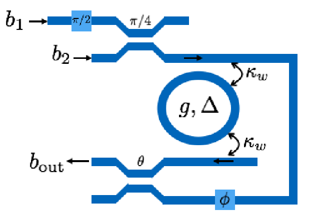
For $Q\sim 10^{4}$, the transient response of an AND gate implemented with both $\chi^{(2)}$ and $\chi^{(3)}$ nonlinearities is shown in Fig. 3(b). Clearly, at quality factors of this order of magnitude the input power ($P_{\text{in}}\sim\hbar\omega_{1}b_{0}^{2}$) required for a $\chi^{(3)}$ based design is $\sim 20$ times larger than that required for a $\chi^{(2)}$ based design. However, we also note from Fig. 3(c) that for designs operating at the same input power, the $\chi^{(3)}$ AND gate shows a larger SNR as compared to the $\chi^{(2)}$ AND gate. This can be attributed to the noise being added to the second harmonic mode in the $\chi^{(2)}$ nonlinear cavity ($\sqrt{2\kappa_{2}}\eta_{2}(t)$ in Eq. 1b). On the other hand, the cavity quality factor required to design a $\chi^{(3)}$ AND gate operating at low input power is significantly higher as compared to those required by the $\chi^{(2)}$ AND gate. For instance, it can be seen from Fig. 3(d) that the $\chi^{(2)}$ AND gate designed with $Q\sim 10^{4}$ can operate at an input power of $\sim 10\ \mu$W with an SNR of $\sim$ 20 dB whereas the $\chi^{(3)}$ AND gate requires $Q\sim 10^{5}$ to operate at similar input powers even though it offers a significantly higher SNR ($\sim 30$ dB).

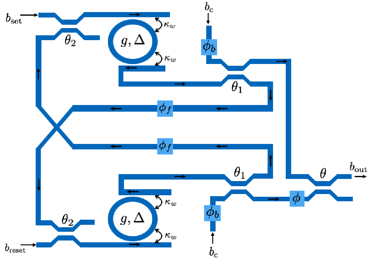
A bistable latch can be designed by combining two cavities in feedback (Fig. 4(a)) [7, 8]. The latch state is governed by two inputs $b_{\text{set}}$ and $b_{\text{reset}}$ – if $(b_{\text{set}},b_{\text{reset}})\equiv(\text{HIGH},\text{LOW})$, the latch output is pulled up to HIGH, if $(b_{\text{set}},b_{\text{reset}})\equiv(\text{LOW},\text{HIGH})$ the latch output is pulled down to LOW and when $(b_{\text{set}},b_{\text{reset}})\equiv(\text{HIGH},\text{HIGH})$ the output is held at its previous value. The parameters $\theta$ and $\phi$ of the final directional coupler and phase-shifter can be chosen so as to achieve equal output amplitudes during both a latch set and the following hold, and a latch reset and the following hold. Additionally, the circuit parameters $\theta_{1},\theta_{2},\phi_{b},\phi_{f}$ and the field $b_{c},b_{0}$ ($b_{0}$ being the input high level) need to be chosen so as to ensure that the overall circuit exhibits bistability during the hold condition ($(b_{\text{set}},b_{\text{reset}})\equiv(\text{HIGH},\text{HIGH})$) – this is desired since the circuit output during a hold is a function of the previous state of the latch and not dependent solely on the circuit inputs ($b_{\text{set}},b_{\text{reset}}$). To achieve this, we numerically maximize the ratio of the output magnitude when the latch holds a HIGH value to the output magnitude when the latch holds a LOW value as a function of $(\theta_{1},\theta_{2},\phi_{b},\phi_{f},b_{c},b_{0})$. The cascadability of the output signal also requires the phase of the output to be equal both when the latch is set and when it holds a HIGH data and when the latch is reset and when it holds a LOW data. This is an additional constraint that we impose while optimising the circuit parameters so as to achieve a bistable latch circuit.

Fig. 4(b) shows a transient simulation of the latch circuit designed with both $\chi^{(2)}$ and $\chi^{(3)}$ nonlinearities at $Q\sim 10^{4}$. At quality factors of this order of magnitude, the $\chi^{(2)}$ based design operates at an input power ($P_{\text{in}}\sim\hbar\omega_{1}(b_{0}^{2}+b_{c}^{2})$) which is $\sim 20$ times smaller than that of the $\chi^{(3)}$ based design. As with the AND gate, we observe that the latch implemented with $\chi^{(3)}$ nonlinearity offers better noise performance compared to the latch implemented with $\chi^{(2)}$ nonlinearity (Fig. 4(c)) for the same input power with the tradeoff being the requirement of significantly larger quality factors (Fig. 4(d)) – the latch designed with $\chi^{(3)}$ nonlinearity requires $Q\sim 10^{5}-10^{6}$ to operate at input powers $\sim 10\ \mu$W whereas the corresponding design with $\chi^{(2)}$ nonlinearity requires $Q\sim 10^{4}$ to operate at similar input powers.

We analyze and compare the power consumption and noise performance of all-optical logic gates (AND gate, latch) implemented using networks of optical cavities with $\chi^{(2)}$ and $\chi^{(3)}$ nonlinearities. Using realistic estimates for the achievable nonlinear coupling constants, it is shown that the $\chi^{(2)}$ based photonic circuits are orders of magnitude more energy efficient as compared to the $\chi^{(3)}$ based photonic circuits at achievable quality factors ($Q\sim 10^{4}$). This is verified by simulating an optical AND gate and an optical latch implemented using both the nonlinearities. The quantum noise in the implemented circuits is simulated using stochastic models derived from the Wigner quasi-probability distribution function. We observe that, for the same input power, optical gates implemented with $\chi^{(3)}$ nonlinearity have larger output SNR as compared to the optical gates implemented with $\chi^{(2)}$ nonlinearity. However, optical logic gates with $\chi^{(2)}$ nonlinearity can achieve low-power operation at significantly smaller quality factors as compared to optical logic gates with $\chi^{(3)}$ nonlinearity thereby making them a more suitable candidate to reduce the overall power consumption of photonic logic circuits.

References

- [1] D Cotter, RJ Manning, KJ Blow, AD Ellis, AE Kelly, D Nesset, ID Phillips, AJ Poustie, and DC Rogers. Science, 286(5444):1523–1528, 1999.
- [2] David AB Miller. Nature Photonics, 4(1):3–5, 2010.
- [3] A Imamoḡlu, Helmut Schmidt, Gareth Woods, and Moshe Deutsch. Physical Review Letters, 79(8):1467, 1997.
- [4] Arka Majumdar and Dario Gerace. Physical Review B, 87(23):235319, 2013.
- [5] Yifang Chen. Microelectronic Engineering, 135:57–72, 2015.
- [6] Ivo Utke, Stanislav Moshkalev, and Phillip Russell. Nanofabrication using focused ion and electron beams: principles and applications. Oxford University Press, 2012.
- [7] Charles Santori, Jason S Pelc, Raymond G Beausoleil, Nikolas Tezak, Ryan Hamerly, and Hideo Mabuchi. Physical Review Applied, 1(5):054005, 2014.
- [8] Hideo Mabuchi. Applied Physics Letters, 99(15):153103, 2011.
- [9] M Dinu, F Quochi, and H Garcia. Applied Physics Letters, 82(18):2954–2956, 2003.
- [10] Alan D Bristow, Nir Rotenberg, and Henry M Van Driel. Appl. phys. lett, 90(19):191104, 2007.
- [11] Jan Niehusmann, Andreas Vörckel, Peter Haring Bolivar, Thorsten Wahlbrink, Wolfgang Henschel, and Heinrich Kurz. Optics letters, 29(24):2861–2863, 2004.
- [12] Parag B Deotare, Murray W McCutcheon, Ian W Frank, Mughees Khan, and Marko Lončar. Applied Physics Letters, 94(12):121106, 2009.
- [13] Ichiro Shoji, Takashi Kondo, Ayako Kitamoto, Masayuki Shirane, and Ryoichi Ito. JOSA B, 14(9):2268–2294, 1997.
- [14] S Bergfeld and W Daum. Physical review letters, 90(3):036801, 2003.
- [15] J Sweet, BC Richards, JD Olitzky, J Hendrickson, G Khitrova, HM Gibbs, D Litvinov, D Gerthsen, DZ Hu, DM Schaadt, et al. Photonics and Nanostructures-Fundamentals and Applications, 8(1):1–6, 2010.
- [16] Sylvain Combrié, Alfredo De Rossi, Quynh Vy Tran, and Henri Benisty. Optics letters, 33(16):1908–1910, 2008.
- [17] Vilson R Almeida and Michal Lipson. Optics letters, 29(20):2387–2389, 2004.
- [18] Kengo Nozaki, Akihiko Shinya, Shinji Matsuo, Yasumasa Suzaki, Toru Segawa, Tomonari Sato, Yoshihiro Kawaguchi, Ryo Takahashi, and Masaya Notomi. Nature Photonics, 6(4):248–252, 2012.
- [19] Kengo Nozaki, Akihiko Shinya, Shinji Matsuo, Tomonari Sato, Eiichi Kuramochi, and Masaya Notomi. Optics express, 21(10):11877–11888, 2013.
- [20] Kengo Nozaki, Takasumi Tanabe, Akihiko Shinya, Shinji Matsuo, Tomonari Sato, Hideaki Taniyama, and Masaya Notomi. Nature Photonics, 4(7):477–483, 2010.
- [21] Majid Sodagar, Mehdi Miri, Ali A Eftekhar, and Ali Adibi. Optics express, 23(3):2676–2685, 2015.
- [22] Arka Majumdar and Armand Rundquist. Optics letters, 39(13):3864–3867, 2014.
- [23] Fabrizio Bonani and Giovanni Ghione. Solid-State Electronics, 43(2):285–295, 1999.
- [24] Kerry Vahala and Amnon Yariv. Quantum Electronics, IEEE Journal of, 19(6):1102–1109, 1983.
- [25] John Gough and Matthew R James. Automatic Control, IEEE Transactions on, 54(11):2530–2544, 2009.
- [26] SJ Carter. Physical Review A, 51(4):3274, 1995.
- [27] Leonard Mandel and Emil Wolf. Optical coherence and quantum optics. Cambridge university press, 1995.
- [28] Howard Carmichael. An open systems approach to quantum optics: lectures presented at the Université Libre de Bruxelles, October 28 to November 4, 1991, volume 18. Springer Science & Business Media, 2009.
- [29] CW Gardiner and MJ Collett. Physical Review A, 31(6):3761, 1985.
- [30] Crispin Gardiner and Peter Zoller. Quantum noise: a handbook of Markovian and non-Markovian quantum stochastic methods with applications to quantum optics, volume 56. Springer Science & Business Media, 2004.
- [31] Yoshihiro Saito and Taketomo Mitsui. SIAM Journal on Numerical Analysis, 33(6):2254–2267, 1996.
- [32] H Lamba, Jonathan C Mattingly, and Andrew M Stuart. IMA journal of numerical analysis, 27(3):479–506, 2007.
- [33] Taylor K Fryett, Christopher M Dodson, and Arka Majumdar. Optics express, 23(12):16246–16255, 2015.
- [34] Sara Ferretti and Dario Gerace. Physical Review B, 85(3):033303, 2012.