Gravitational localization of scalar zero modes in branes
Abstract
The fluctuations of 5D self-gravitating non-abelian kinks which arise from the breaking of the symmetric theory are analyzed within the context of brane-worlds. While tensor and vector sectors of these fluctuations behave like its counterparts in the standard abelian kinks, the mixing between the field excitations of the non-abelian kink and the scalar components of the metric makes the pure scalar sector of the theory very interesting. The spectrum of these scalar fluctuations, which includes gravitationally trapped massless modes on the core of the wall associated to the broken symmetries, is discussed for the two classes of kinks that break to its maximal subgroups.
pacs
11.27.+d, 04.50.-hI Introduction
The central idea in brane-world scenarios is that matter and its interactions, as we know them, must be localized on the brane. Domain wall spacetimes, providing regularizations of the Randall-Sundrum brane-world [1, 2] preserve the property of produce effective 4D gravity on the brane [3, 4, 5, 6]. In addition, while it has been shown that fermion fields may be localized on the brane via their interaction with the scalar field from which the wall is made of [7, 8, 9, 10, 11, 12, 13], gauge field localization has been somewhat more elusive [14, 15, 16, 17, 18, 19, 20].
A lot of work has been done on the topic of localization in brane-worlds in which the field theoretic domain walls considered arise in abelian -symmetric theories, although it is also possible to consider (besides the symmetry) continuos internal symmetry walls with interesting localization properties. There are well known examples of domain walls in flat space-time that arise in a symmetric theory [21, 22, 23, 24] in which the full symmetry is not restored at the core of the wall [25]. This makes non-abelian domain walls of this sort (rather its extensions to the gravitating case) very interesting within the context of brane-worlds [25, 26, 27, 28].
It has been shown that non-abelian branes in flat space that break to may produce, via the Dvali-Shifman (DS) mechanism [29], an effective theory on the brane [27]. On the other hand, self-gravitating domain walls, supporting 4D massless fermion excitations in its world volume, may also localize 4D massless non-abelian excitations via the DS mechanism, depending of the symmetry breaking pattern [28].
While domain walls in abelian -symmetric theories are topologically stable, there is no global stability criterium for the non-abelian ones. This lead us to resort to perturbative analysis, after a solution is found, to establish at least their local stability [23, 24]. Furthermore, the inclusion of gravity makes the perturbative analysis somewhat more intricate than the analogous one in flat spacetime due to the mixing between the field excitations of the non-abelian kink and the scalar components of the metric , in a theory invariant under diffeomorphisms acting both on the and on .
In this work we make a perturbative analysis for the 5D self-gravitating domain walls of [28] in terms of diffeomorphism-invariant quantities. This analysis not only shows that these walls are perturbatively stable, it also permits to study the gravitationally trapped content from the point of view of 4D observers localized on the brane. We find, as expected, that the tensor and vector sectors of the fluctuations behave as its counterparts in the more familiar -symmetric domain walls. On the other hand, the scalar sector of the fluctuations in the case shows a rather different behavior from the abelian one, being linked to the particular symmetry breaking pattern considered and with a spectrum that includes normalizable massless modes, i.e., with massless scalar particles associated to the broken symmetries which are gravitationally trapped on the core of the wall.
II Self-gravitating kinks
In this section we briefly recall the results of [28] regarding the properties of 5D selfgravitating domain walls formed in the two possible symmetry breaking patterns of . Let us consider the -dimensional theory
| (1) |
where is the scalar curvature, is the determinant of the metric, is a scalar field that transforms in the adjoint representation of and a potential such that (1) is invariant under the transformations
- •
, ,
- •
,
where , are traceless hermitian generators of .11 1 We use units were
The Einstein-scalar field equations for this system are
| (2) |
where
| (3) |
and
| (4) |
where . Exact domain wall solutions of (2,3,4) are available for a sixth-order Higgs potential of the form
| (5) | |||||
for special values of the couplings which yield integrable models.
Assuming that the geometry preserves 4D-Poincare invariance, the metric ansatz is
| (6) |
with and a domain wall solution of the form
| (7) |
is proposed, where satisfy the boundary conditions
| (8) |
with and appropriately chosen orthogonal diagonal generators of .
Imposing the integrability conditions
| (9) |
| (10) |
for the special values of the couplings given by
| (11) |
an exact domain wall solution is given by [28]
| (12) |
where , y can be written explicitly in terms of and , and is a numerical constant which depends on the choice of and . On the other hand,
| (13) |
and the space-time is asymptotically with cosmological constant .
As discussed in [28] (see [23, 24] for the flat space case), the choice of and relies on the desired asymptotic values for at . It is well known that in flat space-time there are two symmetry breaking patterns of by a field in the adjoint, involving the breaking to subgroups with the same rank as and occurring as minima of a fourth-order potential [30, 31]. These are
| (14) |
and
| (15) |
the second type of symmetry breaking pattern yielding the largest residual symmetry. In the remainder of this section, we quote the results of [28] concerning to the symmetry breakings (14) and (15) for the gravitating case with the sixth order potential and refer the reader to that work for a detailed discussion on these and the other issues related to localization of fermions and gauge fields within the context of brane-worlds.
II.1 Symmetry breaking
For this symmetry breaking pattern we have
| (16) |
| (17) |
and . With and the unbroken symmetries at and , respectively, we have
| (18) |
| (19) |
with the following embeddings
| (20) |
in the sense that the Cartan subalgebra de () is a subspace of the Cartan-subalgebra space of () corresponding to the particular basis chosen for the Lie algebra. resembles the gauge group on which is based the Higgs sector of the minimal 4D Left-Right symmetric theory. This 5D non-abelian wall may be thought as the generalization to the gravitating case of the perturbatively stable flat space one for a quartic potential of the references [22, 23, 24].
II.2 Symmetry breaking
In this case,
| (21) |
| (22) |
and . The unbroken symmetries are
| (23) |
| (24) |
where is embedded in diferent manners in and . In this symmetry breaking pattern, the gauge bosons on the wall need to form massive glueballs of in order to escape into the bulk, so they can be localized on the wall via the Dvali-Shifman mechanism [29].
III Diffeomorphism-invariant fluctuations
Let and be the metric and the scalar field solutions of the field equations of the theory (1). Let and the metric and scalar field fluctuations, respectively, around the above background. Following [6] we find that these fluctuations satisfy
| (25) |
and
| (26) | |||||
where and
| (27) |
For the theory (1) with the sixth order potential (5) we have
| (28) | |||||
and
| (29) | |||||
In the background provided by the kinks discussed in the previous section, (28) reduces to
| (30) |
and the right hand side of (29) turns out diagonal in . However, although they get notably simplified, (25) and (26) are still extremely involved.
Indeed, as is well known, and are not diffeomorphism invariant variables. Under an infinitesimal diffeomorphism of the form
| (31) |
we have
| (32) |
and
| (33) |
where and describe the same physical perturbations. Hence we must take care of the general coordinate invariance of the theory (1).
Since the background provided by the kinks preserves 4D-Poincare invariance, we decompose (from the point of view of the 4-dimensional observers confined to the wall) in scalar, vector and tensor sectors. Following [32], we set
| (34) |
| (35) |
and
| (36) |
where
| (37) |
and
| (38) |
From (32), with
| (39) |
where
| (40) |
we have that under an infinitesimal diffeomorphism
| (41) |
| (42) |
| (43) |
and
| (44) |
and from (33) we have
| (45) |
The sector is automatically diffeomorphism invariant, i.e. , while it is also possible to define an invariant divergenceless vector (since we have one vector gauge function )
| (46) |
and two diffeomorphism invariant scalar fluctuations (since we have two gauge functions y ) given by
| (47) |
and
| (48) |
such that , and .
On the other hand for the diffeomorphism invariant non-abelian scalar field fluctuation we find
| (49) |
such that .
In the (generalized) longitudinal gauge [32], and , the freedom of the coordinate transformations (31) is completely fixed and we have , , and . This leaves us with the tensor , vector and scalar sectors which decouple from each other at the linearized level.
The tensor and vector sectors of the fluctuations behave as their corresponding analogous in the standard abelian kinks, widely discussed in the literature. It is the scalar sector of the theory under consideration that is quite different from the case. Nevertheless, in order to render this work self-consistent, we will also discuss briefly the tensor and vector fluctuations. In the following, the results will be expressed in the conformal coordinate
| (50) |
such that
| (51) |
III.1 Tensor fluctuations
In the tensor sector with , the modes , satisfy the Schrödinger-like equation
| (52) |
where
| (53) |
and . supports a massless bound state which can be identified with the graviton and a tower of non-normalizable massive states which propagate in the bulk. As is well known, the above equation can be factorized as
| (54) |
which implies the absence of modes with , ensuring the stability of the system under tensor perturbations. As in the abelian kink [33], the normalizable massless tensor mode is given by which reproduces 4D gravity on the core of the wall, while the continuum of massive modes gives small corrections to this behavior at short distances.
III.2 Vector fluctuations
III.3 Scalar fluctuations
In the scalar sector we have the set of diffeomorphism-invariant fluctuations , which are subject to two constraints. The first one only involves scalars without charge under and is given by
| (57) |
while the second one involves also the component of
| (58) |
From (57) and (58) it follows that the fluctuations , and are not independent and correspond to a single physical scalar fluctuation.
With , the modes satisfy
| (59) |
where is given by
| (60) |
does not support normalizable massless states. Notice that
| (61) |
where
| (62) |
implying the absence of modes with . This scalar fluctuation has an exact analogous one in the abelian selfgravitating kink (see [32]).
Now, let us consider the scalar fluctuation . Let with
| (63) |
The modes satisfy Schrödinger-like equations which depends on .
First, let us consider perturbations along the direction. For , (it should be recalled that the fluctuations , and are not independent) satisfy
| (64) |
where is given by
| (65) | |||||
In terms of , as defined in (62), (64) can be rewritten as
| (66) |
and from (61) and (66), it follows that the eigenvalues of the modes of and always come in pairs, except possibly for the massless ones. Hence there are no modes with for . On the other hand, the massless solution of (64) is given by
| (67) |
which is however no normalizable since is not bounded for . This is the mode which is expected to be related, when gravity is switched off, to the translational zero mode of the flat space kink [22, 23, 24]. As in the abelian kinks [5, 34], once we include gravity, the massless mode is no normalizable and therefore no localized.
The behavior of the scalar fluctuation close parallels the one of the scalar fluctuation associated to the standard abelian kink [32]. Now, let us consider perturbations along the other generators of different from . For , satisfy
| (68) |
where is given by
| (69) |
with given by (53).
For , we find
| (70) |
for both symmetry breakings. is everywhere positive and hence does not support bound states with . As expected, is stable to perturbations along the direction. Furthermore, these perturbations do not generate normalizable 4D massless modes independently of the symmetry breaking pattern.
For a generator of and , we find for the symmetry breaking A
| (71) |
where is the function defined by
| (72) |
with (50). These are perturbations along the six generators of , the signs correspond to the two different . On the other hand, for the symmetry breaking B we find
| (73) |
for the perturbations along the eight generators of . In both symmetry breaking patterns, is everywhere positive and hence does not support bound states with . From the above results, it follows that perturbations along the generators of do not generate normalizable 4D massless modes.
Next, let us consider perturbations along those generators of that are not generators of , which will be called broken generators. For a perturbation along such that is a generator of but not of (plus signs) or a generator of but not of (minus signs), we find for the symmetry breaking A
| (74) |
and for the symmetry breaking B
| (75) | |||||
These ones are perturbations along the generators that are broken only at one side of the wall, with for the symmetry breaking A and for the symmetry breaking B ( is the dimension of the coset ). The Schrödinger-like equation for these fluctuations can not be written in terms of a fake superpotential as we did for . However, on general grounds and from the shape of for these perturbations (see Fig.1), besides a mild resonance behavior, trapped massless modes are expected.
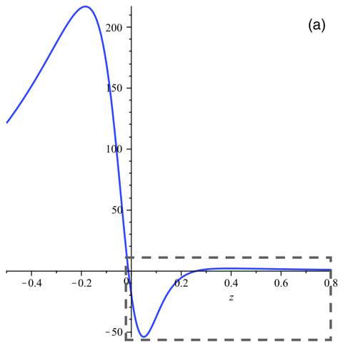
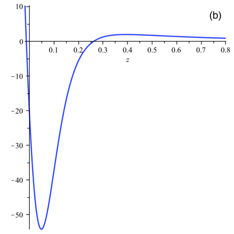
These gravitationally trapped massless modes correspond to rotations of within the class described by . In the non-gravitating setting the analogous zero modes behave as and are not normalizable [23]. Hence, gravitationally trapped massless modes associated to these perturbations can be seen as the zero modes in flat space which turn out normalizable and get localized once we include gravity. For this type of perturbations there are no bound states in the flat space case [23], we find no modes with neither in the gravitating case.
Finally, for such that is not a generator of nor of , we find that and the modes satisfy
| (76) |
As stated above, supports a massless bound state, a tower of non-normalizable massive states with and no modes with . These ones are perturbations along the generators that are broken everywhere, with for the symmetry breaking A and for the symmetry breaking B.
The above results show that the 5D self-gravitating domain walls of [28] are perturbatively stable. Additionally, on both symmetry breaking patterns, normalizable 4D massless modes of the kink fluctuations appear when is not a generator of . The existence of normalizable massless scalar modes is reminiscent of the situation envisaged in [35], although in the latter these modes appears in abelian -symmetric models with scalar fields () and a potential generated by a fake superpotential.
IV Summary and Outlook
Dynamical localization of gauge fields via the DS-mechanism [29] in non-abelian domain wall scenarios has been put forward in [26, 25] and discussed in [27] for a flat space model based on a symmetry group and in [28] for a gravitating model. Besides the fact that the stability of non-abelian kinks is not guaranteed and should be proved at least perturbatively [23, 24], it is clear that the 4D phenomenology on the brane may be influenced by the inclusion of gravity which couples metric fluctuations with the wall fluctuations.
We have thus carried out a diffeomorphism-invariant analysis of the fluctuations of the 5D self-gravitating domain walls of [28], in order to determine their perturbative stability as well as their localization properties from the point of view of 4D observers.
We find no modes with for the fluctuations of the self-gravitating kinks, implying that these are perturbatively stable as in the flat space-time case [22, 23, 24].
Not surprisingly, the tensor and vector sectors of the fluctuations behave in the same way as the corresponding ones of the standard kinks. There is a normalizable massless mode in the tensor sector which gives rise to 4D gravity on the brane and a tower of non-normalizable massive states which propagate in the bulk. There is no localized vector fluctuation.
On the other hand, the scalar sector of the fluctuations for the self-gravitating kinks greatly differs from its analogous for the abelian case. We find no normalizable 4D massless modes associated to the unbroken subgroup on the core of the wall, independently of the symmetry breaking pattern considered. However, there are as many normalizable 4D zero modes as there are broken generators, i.e., we find gravitationally localized massless 4D scalar particles without charge under which can be identified as (the 4D zero modes of) the Nambu-Goldstone fields associated to the symmetry breaking . This gravitational trapping of Nambu-Goldstone bosons is presumably shared with other non-abelian domain-walls, a subject that deserves a further separate investigation.
V Acknowledgements
We wish to acknowledge fruitful discussions with Adel Khoudeir, Alejandra Melfo and Aureliano Skirzewski.
References
- [1] L. Randall, R. Sundrum, Phys. Rev. Lett. 83 (1999) 4690-4693. [hep-th/9906064].
- [2] R. Guerrero, A. Melfo and N. Pantoja, Phys. Rev. D 65 (2002) 125010 [gr-qc/0202011].
- [3] O. DeWolfe, D. Z. Freedman, S. S. Gubser, A. Karch, Phys. Rev. D62 (2000) 046008. [hep-th/9909134].
- [4] M. Gremm, Phys. Lett. B478 (2000) 434-438. [hep-th/9912060].
- [5] Z. Kakushadze, P. Langfelder, Mod. Phys. Lett. A15 (2000) 2265-2280. [hep-th/0011245].
- [6] O. Castillo-Felisola, A. Melfo, N. Pantoja, A. Ramirez, Phys. Rev. D70 (2004) 104029. [hep-th/0404083].
- [7] B. Bajc, G. Gabadadze, Phys. Lett. B474 (2000) 282-291. [hep-th/9912232].
- [8] A. Kehagias, K. Tamvakis, Phys. Lett. B504 (2001) 38-46. [hep-th/0010112].
- [9] C. Ringeval, P. Peter, J. -P. Uzan, Phys. Rev. D65 (2002) 044016. [hep-th/0109194].
- [10] R. Koley, S. Kar, Class. Quant. Grav. 22 (2005) 753-768. [hep-th/0407158].
- [11] A. Melfo, N. Pantoja, J. D. Tempo, Phys. Rev. D73 (2006) 044033. [hep-th/0601161].
- [12] Y. -X. Liu, C. -EFu, L. Zhao, Y. -S. Duan, Phys. Rev. D80 (2009) 065020. [arXiv:0907.0910 [hep-th]].
- [13] R. Guerrero, A. Melfo, N. Pantoja, R. O. Rodriguez, Phys. Rev. D74 (2006) 084025. [hep-th/0605160].
- [14] S. J. Huber and Q. Shafi, Phys. Rev. D 63 (2001) 045010 [arXiv:hep-ph/0005286].
- [15] G. R. Dvali, G. Gabadadze and M. A. Shifman, Phys. Lett. B 497, 271 (2001) [arXiv:hep-th/0010071].
- [16] S. L. Dubovsky, V. A. Rubakov, Int. J. Mod. Phys. A16 (2001) 4331-4350. [hep-th/0105243].
- [17] B. Batell, T. Gherghetta, Phys. Rev. D75 (2007) 025022. [hep-th/0611305].
- [18] R. Guerrero, A. Melfo, N. Pantoja, R. O. Rodriguez, Phys. Rev. D81 (2010) 086004. [arXiv:0912.0463 [hep-th]].
- [19] A. E. R. Chumbes, J. M. Hoff da Silva and M. B. Hott, Phys. Rev. D 85 (2012) 085003 [arXiv:1108.3821 [hep-th]].
- [20] C. Germani, Phys. Rev. D 85 (2012) 055025 [arXiv:1109.3718 [hep-ph]].
- [21] G. R. Dvali, H. Liu, T. Vachaspati, Phys. Rev. Lett. 80 (1998) 2281-2284. [hep-ph/9710301].
- [22] L. Pogosian, T. Vachaspati, Phys. Rev. D62 (2000) 123506. [hep-ph/0007045].
- [23] T. Vachaspati, Phys. Rev. D63 (2001) 105010. [hep-th/0102047].
- [24] L. Pogosian, T. Vachaspati, Phys. Rev. D64 (2001) 105023. [hep-th/0105128].
- [25] T. Vachaspati, Phys. Rev. D 67 (2003) 125002 [hep-th/0303137].
- [26] A. Davidson, B. F. Toner, R. R. Volkas and K. C. Wali, Phys. Rev. D 65 (2002) 125013 [hep-th/0202042].
- [27] A. Davidson, D. P. George, A. Kobakhidze, R. R. Volkas and K. C. Wali, Phys. Rev. D 77 (2008) 085031 [arXiv:0710.3432 [hep-ph]].
- [28] A. Melfo, R. Naranjo, N. Pantoja, A. Skirzewski and J. C. Vasquez, Phys. Rev. D 84 (2011) 025015 [arXiv:1104.4857 [hep-th]].
- [29] G. R. Dvali, M. A. Shifman, Phys. Lett. B396 (1997) 64-69. [hep-th/9612128].
- [30] L. F. Li, Phys. Rev. D 9 (1974) 1723.
- [31] N. Chen, T. A. Ryttov and R. Shrock, Phys. Rev. D 82 (2010) 116006 [arXiv:1010.3736 [hep-ph]].
- [32] M. Giovannini, Phys. Rev. D 64 (2001) 064023 [hep-th/0106041].
- [33] P. Callin and F. Ravndal, Phys. Rev. D 70 (2004) 104009 [arXiv:hep-ph/0403302].
- [34] M. Shaposhnikov, P. Tinyakov and K. Zuleta, JHEP 0509 (2005) 062 [hep-th/0508102].
- [35] D. P. George, Phys. Rev. D 83 (2011) 104025 [arXiv:1102.0564 [hep-th]].