Bases for cluster algebras from orbifoldsThanks: AF was partially supported by EPSRC grant EP/N005457/1
Abstract.
We generalize the construction of the bracelet and bangle bases defined in [MSW2] and the band basis defined in [T2] to cluster algebras arising from orbifolds. We prove that the bracelet bases are positive, and the bracelet basis for the affine cluster algebra of type is atomic. We also show that cluster monomial bases of all skew-symmetrizable cluster algebras of finite type are atomic.
1. Introduction
Cluster algebras were introduced by Fomin and Zelevinsky [FZ1] in the effort to understand a construction of canonical bases by Lusztig [L] and Kashiwara [K]. A cluster algebra is a commutative ring with a distinguished set of generators called cluster variables. Cluster variables are grouped into overlapping finite collections of the same cardinality called clusters connected by local transition rules which are determined by a skew-symmetrizable exchange matrix associated with each cluster, see Section 2 for precise definitions.
One of the central problems in cluster algebras theory is a construction of good bases. It was conjectured in [FZ1] that these bases should contain cluster monomials, i.e. all products of cluster variables belonging to every single cluster. Linear independence of cluster monomials in skew-symmetric case was proved by Cerulli Irelli, Keller, Labardini-Fragoso and Plamondon in [CKLP], for a general skew-symmetrizable case linear independence was recently proved by Gross, Hacking, Keel and Kontsevich in [GHKK]. In the finite type cluster monomials themselves form a basis (Caldero and Keller [CK]).
Bases containing cluster monomials were constructed for various types of cluster algebras. These include ones by Sherman and Zelevinsky [SZ] (rank two affine type), Cerulli Irelli [C1] (affine type ), Ding, Xiao and Xu [DXX] (affine type), Dupont [D1, D3], Geiss, Leclerc and Schröer [GLS], Plamondon [Pl] (generic bases for acyclic types), Lee, Li and Zelevinsky (greedy bases in rank two algebras).
In [MSW2] Musiker, Schiffler and Williams constructed two types of bases (bangle basis and bracelet basis ) for cluster algebras originating from unpunctured surfaces [FST, FT, FG1]. A band basis (we call it ) was introduced by D. Thurston in [T2]. All the three bases are parametrized by collections of mutually non-intersecting arcs and closed loops, and all their elements are positive, i.e. the expansion of any basis element in any cluster is a Laurent monomial with non-negative coefficients.
In the present paper, we extend the construction of all the three bases to cluster algebras originating from orbifolds.
Theorem 1.1.
Let be a cluster algebra with principal coefficients constructed by an unpunctured orbifold with at least two boundary marked points. Then , and are bases of .
Our main tools are the tropical duality by Nakanishi and Zelevinsky [NZ], and the theory of unfoldings developed in [FeSTu2, FeSTu3]. The notion of an unfolding was introduced by Zelevinsky, it provides a reduction of problems on (certain) skew-symmetrizable cluster algebras to appropriate skew-symmetric ones. In our case, unfoldings allow us to treat cluster algebras from orbifolds using the results known for cluster algebras from surfaces, in particular, to use the results of [MSW2].
The tropical duality provides a relation between -vectors and -vectors of a cluster algebra with principal coefficients. For cluster algebras originating from surfaces and orbifolds, the -vectors have an explicit geometric meaning: they can be viewed as collections of shear coordinates of specially constructed laminations [FG2, FG3, FT]. To prove linear independence of the constructed bases, -vectors are used in [MSW2]. We use tropical duality together with results of [FeSTu3] to supply -vectors with geometric meaning: they can be read off from shear coordinates of some laminations on a dual orbifold.
We also consider positivity properties of the constructed bases. A basis of cluster algebra is called positive if it has positive structure constants. Positivity of for surfaces was conjectured in [FG1] and proved in [T2]. We extend this result to the orbifold case.
Theorem 9.2.
The bracelet basis is positive.
The bangle basis is not positive as shown in [T1], the band basis is conjectured to be positive [T2].
A basis is called atomic if it satisfies the following property: non-negative linear combinations of basis elements are exactly those elements of the algebra whose Laurent expansion is positive in any cluster. If it exists, atomic basis is unique [SZ]. It is proved in [C2] (see also [CL]) that the cluster monomial bases of skew-symmetric cluster algebras are atomic. We extend this result to the full generality.
Theorem 10.2.
Cluster monomial bases of skew-symmetrizable cluster algebras of finite type are atomic.
The bracelet basis for surfaces was conjectured to be atomic in [MSW2]. In particular, the atomic basis for constructed in [DT] is precisely the bracelet basis for an unpunctured annulus with and points at the boundary components. We use unfoldings to prove the following result.
Theorem 10.3.
The bracelet basis of the cluster algebra of the affine type is atomic.
Recently, Gross, Hacking, Keel and Kontsevich [GHKK] constructed a canonical positive theta basis for every cluster algebra of geometric type. An interesting question is the relation between the theta bases and the bases constructed in [MSW2] and the present paper. The theta basis cannot coincide with the bangle basis since the latter is not positive. According to [CGMMRSW], theta bases of cluster algebras of rank two coincide with greedy bases. In particular, for affine algebra the theta basis is precisely the bracelet basis (and not the band basis). Is this always the case, i.e. does the bracelet basis coincide with the theta basis for all surfaces and orbifolds?
We also note that all the bases in [MSW2] were constructed for unpunctured surfaces with at least two boundary marked points. It was shown in [CLS] that the results of [MSW2] also hold for unpunctured surfaces with a single boundary marked point. Following [CLS], one can show that the results of the current paper can also be extended to orbifolds with a single boundary marked point, the proof to appear in [CT].
The paper is organized as follows.
In preparatory Sections 2 and 3 we recall basic notions on cluster algebras and remind the construction of cluster algebras from triangulated bordered surfaces and orbifolds.
In Section 4 we define an orbifold unfolding as a ramified covering branching in the orbifold points only. As it was mentioned above, making use of unfoldings is one of our main tools in this paper. However, this only works when all curves in consideration “lift well” in the unfolding. We introduce the notion of a curve which lifts well in a given unfolding and show that for each curve of our interest there exists an unfolding where the curve lifts well. This technical statement is crucial for our proofs.
In Section 5 we build the skein theory for the orbifold case. Section 6 is devoted to the construction of bracelet, band and bangle bases , and for the cluster algebras from orbifolds. We use tropical duality to prove that these sets are bases in Sections 7 and 8.
In Section 9 we discuss positivity property of the bracelet basis . Finally, in Section 10 we show that the bracelet basis for affine cluster algebra of type is atomic. We also prove that cluster monomial bases of cluster algebras of types , and are atomic.
Acknowledgements
We would like to thank G. Musiker, M. Shapiro and D. Thurston for numerous stimulating discussions, and G. Muller and S. Stella for explaining us details of their paper [CGMMRSW]. We are grateful to D. Thurston for his lecture course “Curves on surfaces” in Berkeley, 2012. The paper was partially written in MSRI during the program on cluster algebras. We thank the organizers for the opportunity to participate in the program, and the institute for a nice working atmosphere.
2. Basics on cluster algebras
We briefly remind some definitions and notions introduced by Fomin and Zelevinsky in [FZ1] and [FZ2].
2.1. Cluster algebras
An integer matrix is called skew-symmetrizable if there exists an integer diagonal matrix , such that the product is a skew-symmetric matrix, i.e., .
Let be a tropical semifield , i.e. an abelian group freely generated by elements with commutative multiplication and equipped with addition defined as
The multiplicative group of is a coefficient group of cluster algebra. is the integer group ring. Define as the field of rational functions in independent variables with coefficients in the field of fractions of . is called an ambient field.
Definition 2.1.
A seed is a triple , where
- •
is a collection of algebraically independent rational functions of variables which generates over the field of fractions of ;
- •
, is an -tuple of elements of called a coefficient tuple of cluster ;
- •
is a skew-symmetrizable integer matrix (exchange matrix).
The part of a seed is called cluster, elements are called cluster variables, the part is called coefficient tuple.
We denote .
Definition 2.2 (seed mutation).
For any , we define the mutation of seed in direction as a new seed in the following way:
| (2.1) |
| (2.2) |
| (2.3) |
We write . Notice that . Two seeds are called mutation-equivalent if one is obtained from the other by a sequence of seed mutations. Similarly one says that two clusters or two exchange matrices are mutation-equivalent.
Notice that exchange matrix mutation (2.1) depends only on the exchange matrix itself. The collection of all matrices mutation-equivalent to a given matrix is called the mutation class of .
Following [FZ2], we define a cluster pattern by assigning to every vertex of an -regular tree with edges labeled by a seed , such that two vertices and are joined by an edge labeled by if and only if . We denote the elements of by
For any skew-symmetrizable matrix an initial seed is a collection , , where is the initial exchange matrix, is the initial cluster, is the initial coefficient tuple.
Cluster algebra associated with the skew-symmetrizable matrix is a subalgebra of generated by all cluster variables of the clusters mutation-equivalent to the initial seed .
Cluster algebra is called of finite type if it contains only finitely many cluster variables. In other words, all clusters mutation-equivalent to initial cluster contain only finitely many distinct cluster variables in total.
Definition 2.3.
A cluster algebra is said to be of finite mutation type if it has finitely many exchange matrices.
An extended exchange matrix is an matrix whose upper matrix is and lower part encodes the coefficient tuple using the formula
In terms of the matrix , the exchange relation 2.3 rewrites as
2.2. Cluster algebras with principle coefficients
A cluster algebra has principle coefficients at a seed if .
In other words, a cluster algebra with principle coefficients is associated to a matrix , whose upper part is and the lower (coefficient) part is identity matrix.
A cluster algebra with principle coefficients associated to the matrix is denoted by .
Consider -grading on defined by
where is the standard basis vectors in ( has 1 at -th position and 0 at other places) and is the -th column of .
It is shown in [FZ2] that the Laurent expression of any cluster variable in any cluster of is homogeneous with respect to this -grading. For each cluster variable , the -vector with respect to the seed is the multi-degree of the Laurent expansion of with respect to .
Given the initial seed of and a seed , we denote by the lower part of the exchange matrix (here is the exchange matrix at ). The columns of are called -vectors at , the matrix is called -matrix at . Similarly, we may denote by the matrix composed of -vectors at , i.e. .
According to [NZ, (1.13)], there is a duality between - and -vectors: .
3. Cluster algebras from surfaces and orbifolds
In this section we remind the construction of cluster algebras arising from triangulated surface [FST, FT] and its generalization to the orbifold case [FeSTu3].
Remark 3.1.
In the most part of this paper we work with unpunctured surfaces/orbifolds, so we will not review tagged triangulations and will ignore self-folded triangles (for the details see [FST]).
3.1. Cluster algebras from surfaces
Let be a bordered surface with a finite number of marked points, and with at least one marked point at each boundary component.
A non-boundary marked point is called a puncture. In the most part of this paper we will have no punctures.
An arc is a non-self-intersecting curve with two ends at marked points (may be coinciding) such that
- -
except for its endpoints, is disjoint from the marked points and the boundary;
- -
does not cut out a monogon not containing any marked points;
- -
is not homotopic to a boundary segment.
A triangulation of is a maximal collection of mutually non-homotopic disjoint arcs (two arcs are allowed to have a common vertex).
Given a triangulation of one builds a skew-symmetric signed adjacency matrix as follows:
- •
the rows and columns of correspond to the arcs in ;
- •
let , where for every triangle the number is defined in the following way:
A mutation of the matrix corresponds to a flip of the triangulation in the -th edge, where a flip is a move replacing a diagonal of a quadrilateral by another diagonal, or, more generally, replacing an arc by a unique other arc disjoint from . More precisely, the signed adjacency matrix of the flipped triangulation is .
Introducing a variable for each and using the matrix as initial exchange matrix one can build a cluster algebra .
- •
the algebra does not depend on the initial triangulation chosen in ;
- •
cluster variables of are in bijection with arcs on ;
- •
several cluster variables belong to one cluster if and only if the corresponding arcs belong to one triangulation.
Given a hyperbolic metric on , one can think of marked points as cusps (and thus, the triangles in the triangulation can be thought as ideal triangles). Choose in addition a horocycle around each marked point, and for each arc define as the length of the part of staying away from the horocycles centred in both ends. A lambda length of (as defined in [P]) is .
These functions are subject to Ptolemy relation under the flips:
where and are two diagonals of the quadrilateral with sides . The Ptolemy relation coincides with the exchange relation for cluster variables in , so that cluster variables may be interpreted as lambda lengths, and we will write (as a function of lambda lengths of the arcs in the initial triangulation).
Cluster algebras arising from surfaces are of finite mutation type, moreover, it is shown in [FeSTu1] that all but finitely skew-symmetric cluster algebras of finite mutation type of rank are cluster algebras arising from surfaces.
3.2. Cluster algebras from orbifolds
To obtain (almost all) skew-symmetrizable cluster algebras of finite mutation type one introduces cluster algebras from triangulated orbifolds [FeSTu3].
By an orbifold we mean a triple , where is a bordered surface with a finite set of marked points , and is a finite (non-empty) set of special points called orbifold points, . Some marked points may belong to (moreover, every boundary component must contain at least one marked point; the interior marked points are still called punctures), while all orbifold points are interior points of (later on, as we will supply the orbifold with a metric, the orbifold points will have cone angle ). By the boundary we mean .
An arc in is a curve in considered up to relative isotopy (of ) modulo endpoints such that
- •
one of the following holds:
- –
either both endpoints of belong to (and then is an ordinary arc)
- –
or one endpoint belongs to and another belongs to (then is called a pending arc);
- –
- •
has no self-intersections, except that its endpoints may coincide;
- •
except for the endpoints, and are disjoint;
- •
if cuts out a monogon then this monogon contains either a point of or at least two points of ;
- •
is not homotopic to a boundary segment.
Note that we do not allow both endpoints of to be in .
Two arcs and are compatible if the following two conditions hold:
- •
they do not intersect in the interior of ;
- •
if both and are pending arcs, then the ends of and that are orbifold points do not coincide (i.e., two pending arcs may share a marked point, but neither an ordinary point nor a orbifold point).
A triangulation of is a maximal collection of distinct pairwise compatible arcs. The arcs of a triangulation cut into triangles.
3.2.1. Weights
Each orbifold point of comes with a weight or . A pending arc incident to an orbifold point with weight is assigned with the same weight . An ordinary arc is assigned with the weight . Denote by the weight of -th arc and let
Given a triangulation of one builds a skew-symmetrizable signed adjacency matrix as follows:
- •
the rows and columns of correspond to the arcs in (both ordinary and pending arcs are considered here);
- •
let , where for every triangle the number is defined in the following way:
Introducing a variable for each and using the matrix one can build a cluster algebra .
The geometric realization of is obtained via associated orbifold denoted by . In the associated orbifold, we substitute all weight orbifold points by special marked points and introduce a hyperbolic metric on such that
- •
the marked points (including special marked points) are cuspidal points on ;
- •
the remaining orbifold points (i.e., orbifold points of weight ) are orbifold points with cone angle around each of them equal to ;
- •
the triangles in not incident to special marked points are ideal hyperbolic triangles, the pending arcs of weight understood as two halves of a side of an ideal triangle glued to each other; the pending arcs of weight are called double arcs (in fact, these can be understood as a pair of tagged arcs which are never mutated separately);
- •
each special marked point is endowed with a fixed self-conjugated horocycle, i.e. a horocycle such that the hyperbolic length of equals .
Remark 3.2.
In this paper (except for Section 10) we consider orbifolds without orbifold points of weight . In that case coincides with (where is understood as a union of ideal hyperbolic triangles), so we will omit the word “associated” and will call simply “an orbifold”. Also, by technical reasons, we assume that has at least two marked points.
Now, one can choose in addition an horocycle around each non-special marked point, and for every arc define as the length of the part of staying away from the horocycles centered in both ends (for a pending arc the length is understood as the length of the round trip from a horocycle to the orbifold point and back). The lambda length of is defined as .
It is shown in [FeSTu3] that lambda lengths of arcs satisfy the exchange relations of the cluster algebra , so that they can be interpreted as geometric realizations of cluster variables.
3.3. Coefficients and laminations
In the case of cluster algebras from surfaces or orbifolds, the coefficients can be visualized using laminations (or more precisely, shear coordinates of laminations).
By a lamination on we mean an integral unbounded measured lamination, i.e. a finite collection of non-self-intersecting and mutually disjoint curves on modulo isotopy; every curve here is either a closed curve or a curve each of whose ends is of one of the following three types:
- -
an unmarked point of the boundary of ;
- -
a spiral around a puncture contained in (either clockwise or counter-clockwise);
- -
an orbifold point.
Also, the following is not allowed:
- •
a curve that bounds an unpunctured disc or a disc containing a unique marked, special marked or orbifold point;
- •
a curve with two endpoints on the boundary of isotopic to a piece of boundary containing no marked points or a single marked point;
- •
two curves starting at the same orbifold point (or two ends of the same curve starting at the same orbifold point);
- •
curve spiralling in or starting at any special marked point.
Given a lamination on a surface, the shear coordinates of with respect to a given triangulation (containing no self-folded triangles) were introduced by W. Thurston [T] and can be computed as follows. For each arc of the corresponding shear coordinate of with respect to the triangulation , denoted by , is defined as a sum of contributions from all intersections of curves in with the arc . Such an intersection contributes (resp, -1) to if the corresponding segment of the curve in cuts through the quadrilateral surrounding as shown in Fig. 3.1 on the left (resp, on the right).

The construction is extended to the case of arbitrary (tagged) triangulation of a surface in [FT], and to the case of an orbifold in [FeSTu3]. In particular, the following theorem holds.
Theorem 3.3 ([FeSTu3], Theorem 6.7).
Let be an associated orbifold. For a fixed triangulation of , the map
is a bijection between laminations on and .
A multi-lamination is a finite set of laminations .
Given a multi-lamination and an initial triangulation , compose an extended signed adjacency matrix of the signed adjacency matrix and the matrix of the shear coordinates of in . It appears (see [FT, FeSTu3]) that the transformation of the matrix under a flip coincides with its transformation under the corresponding mutation. This implies that, given a multi-lamination , we can consider shear coordinates of in the triangulation as coefficients in the seed .
In particular, we can keep track of principle coefficients, for which we need elementary laminations. For each arc of a triangulation one can choose the lamination such that and for (it does exist and is unique by Theorem 3.3, in the unpunctured case it may be obtained from the arc by shifting all (non-orbifold) ends clockwise, see Fig. 3.2 for examples).

Composing a multi-lamination of elementary laminations for all curves of , we obtain an extended signed adjacency matrix with the coefficient part . Now we can identify the -matrix at with the matrix of shear coordinates of in the triangulation .
4. Unfoldings and curves on orbifolds
4.1. Orbifold unfoldings
The idea of unfolding was suggested by Andrei Zelevinsky. Roughly speaking, an unfolding of a skew-symmetrizable matrix is a skew-symmetric matrix such that the properties of the cluster algebra can be read off the properties of the cluster algebra (see [FeSTu2, FeSTu3] for details). It turns out that not every skew-symmetrizable algebra has an unfolding, however, in finite mutation type an unfolding almost always exists and proves to be useful. For a cluster algebra from an orbifold an unfolding can be provided by an algebra from a surface, where the surface is a ramified covering of the orbifold branching in the orbifold points only [FeSTu3] and with all ramification indices equal to two. In this paper, we need a notion of a partial unfolding which satisfies some weaker assumptions.
Definition 4.1.
Given an orbifold , a ramified covering of branching in the orbifold points only with all ramification indices equal to two is called a partial unfolding. In addition, is called an unfolding if it contains no orbifold points (or, equivalently, if every orbifold point is a branch point). We supply with a hyperbolic metric such that the covering map is a local isometry everywhere except for the ramification points.
By the degree of a partial unfolding we mean the degree of the covering. In this paper we will only consider partial unfoldings of degree .
By a complete lift of a curve to a partial unfolding we mean the union of all lifts of .
Given a partial unfolding of , each triangulation on lifts to a triangulation on . Moreover, since the covering map is a local isometry, it preserves the lengths of arcs, and thus it preserves lambda lengths (one can note that, due to the definition of a length of pending arc, the covering map also preserves lengths of pending arcs). Therefore, each cluster in lifts to a cluster in (each cluster variable of is a lift of some cluster variable of ). These lifts agree with mutations [FeSTu3] (see also Remark 4.2).
For any function in variables of the cluster by the specialization we mean the function in variables of where each cluster variable of is substituted by its image in .
Remark 4.2.
Let be a degree partial unfolding of , let be a cluster on and be its lift on . Let be an arc or a pending arc on and be a connected component of its lift, . Write as the Laurent expansion in the cluster , and as the Laurent expansions in the cluster .
Then the definitions above imply .
4.2. Curves on orbifolds
Throughout the paper, all curves on surfaces and orbifolds are considered up to isotopy. In particular, every intersection of a family of curves is thought as a simple transversal intersection of two curves. Further, we assume a number of self-intersections of any curve to be finite. By the length of a curve we mean the length of the geodesic representative of the isotopy class.
By a regular point of an orbifold we mean any interior point except for orbifold points.
A curve is called separating if it cuts the surface or orbifold into more than one connected components. Otherwise, it is called non-separating.
We consider several types of curves: with two ends in marked points (possibly coinciding), with one end in a marked point and another in an orbifold point, with two ends in orbifold points (possibly coinciding) or a closed curve. We call these curves an ordinary curve, a pending curve, a semi-closed curve and a closed curve respectively. If the curves of these types are in addition non-self-intersecting we call them an arc, a pending arc, a semi-closed loop and a closed loop (these definitions agree with definitions of arcs and pending arcs given above). Graphically, we denote orbifold points by crosses, their lifts to (partial) unfoldings by small circles and the marked points by bold circles. The curves incident to an orbifold point are drawn thick. We also say that pending curves and semi-closed curves are thick curves and all other types of curves are thin. We summarize the definitions above in Table 4.1.
| curves | non-self-intersecting curves | ||
![[Uncaptioned image]](1511.08023v3/curvedef1.png) |
ordinary curve | arc | thin |
![[Uncaptioned image]](1511.08023v3/curvedef4.png) |
closed curve | closed loop | |
![[Uncaptioned image]](1511.08023v3/curvedef2.png) |
pending curve | pending arc | thick |
![[Uncaptioned image]](1511.08023v3/curvedef3.png) |
semi-closed curve | semi-closed loop |
Remark 4.3.
Remark 4.4.
A curve connecting an orbifold point to itself will be considered as self-intersecting. By closed curves we mean ones not contractible to a point or an orbifold point.
4.3. Curves in unfoldings
Definition 4.5.
Let be a degree partial unfolding of . A closed curve lifts well to if the complete lift of in consists of disjoint closed curves. An ordinary curve, a pending curve and a semi-closed curve are always said to lift well.
Example 4.6.
We show an example of an unfolding and a closed curve which does not lift well. Let be an orbifold of genus with some marked points and precisely two orbifold points, and let be a closed curve on . Take a path connecting two orbifold points and crossing exactly once. We build a degree partial unfolding as follows. Cut the orbifold along , take two copies of the obtained orbifold and glue them together to obtain a connected surface. Then the curve lifts to one closed curve of length (where is the length of ), so it does not lift well.
The following lemma plays the key role in the proof of skein relations for orbifold (see Section 5.5).
Lemma 4.7.
Let be an unpunctured orbifold. Let be a closed curve. Then there exists an unfolding such that lifts well in .
Proof.
In [FeSTu3] we used the following four ways to construct degree two (or four) covering branched in orbifold points only:
- (1)
if the number of orbifold points is even, group orbifold points in pairs, cut the orbifold along mutually non-intersecting semi-closed loops connecting paired orbifold points, take two copies and glue them along the cuts to obtain one surface;
- (2)
if the number of orbifold points is odd and bigger than one, apply (1) to just one pair of orbifold points; this will result in an orbifold with an even number of orbifold points, so (1) can be applied;
- (3)
if there is exactly one orbifold point and the boundary is non-empty, cut the orbifold along a pending arc ending at the boundary, then glue together two copies to obtain a surface;
- (4)
if there is exactly one orbifold point, the boundary is empty, and the genus is positive, construct an unramified degree two covering by cutting the orbifold along a closed non-separating loop and gluing two copies together to double the number of orbifold points, then apply (1).
Note that there is no required covering of closed orbifolds of genus zero with a unique orbifold point.
We now want to combine these to construct a covering where lifts well.
After cutting along the following connected components may appear:
- (i)
contains no orbifold points;
- (ii)
contains orbifold points and at least one boundary component of ;
- (iii)
contains orbifold points, at least one handle and no boundary components of ;
- (iv)
is a disc with orbifold points.
Now our aim is to choose mutually non-intersecting non-self-intersecting paths we cut the orbifold along in such a way that intersects each of them even number of times. This will guarantee that lifts well in the covering. We need to choose such paths to be incident to every orbifold point exactly once, with all other ends being at the boundary marked points. Application of (1) – (4) will then provide a required covering.
First, we connect pairs of orbifold points in the same connected components and make cuts along these paths. This results in at most one orbifold point in every connected component. Next, in all components of type (ii) with one orbifold point, connect this point to a boundary marked point, and make cuts along these paths. In all components of type (iii) with one orbifold point we choose a closed non-separating loop and cut the orbifold along all these loops. Note that all of these cuts do not change connectedness of the connected components of , so this can be done in any order.
We are left to consider discs with one orbifold point each (we do not count holes obtained from the cuts already made). First, we make the following observation: if we take three orbifold points, then we can choose two of them that can be joined by a path intersecting at an even number of points. Thus, if there are more than two discs with one orbifold point each, we can join some pair of orbifold points by a path intersecting an even number of times, make a cut along this path, and then repeat this procedure until at most two orbifold points are left. Denote these points by and . Clearly, and cannot be connected by a path intersecting at an even number of points.
Consider any boundary marked point . Then exactly one of and (say, ) can be connected to by a path intersecting at an even number of points. Connect it to by such a path and cut along it. We are left with one orbifold point only.
Now we take two copies of obtained orbifold and glue them along the cuts. We obtain a partial unfolding of degree two in which lifts well. Assume that is not a surface, otherwise the lemma is already proved.
Denote by the complete lift of . Then any connected component of containing orbifold points is of one of the two types: either contains exactly two orbifold points (these come from connected components of type (iii) with odd number of orbifold points), or is a disc containing one of the lifts of point (denote these two orbifold points by and ). The former ones can be treated as before by cutting along a path between the two points. Let us prove the following statement:
Claim.
Assume that does not coincide with . Then there exists a path connecting to and intersecting each of the two lifts of at an even number of points.
To prove the claim, we look for a closed non-contractible path through satisfying the two conditions:
- -
intersects in an even number of points;
- -
intersects the cuts made on in order to construct an odd number of times.
Then any lift of will connect to and satisfy the assumptions of the claim.
Since does not coincide with , at least one cut was made at the first step. If there was a cut connecting some orbifold point with another orbifold point or a boundary point, then we can take as a loop around based at . If the only cuts were closed loops in connected components of type (iii), then we can choose one such component and take any closed loop in intersecting just one of the cuts exactly once, and then connect this loop to obtaining a loop based at .
Thus, the claim is proved. Note that we may assume does not intersect other cuts we have made on . Cutting along and taking two copies of obtained orbifold, we obtain a degree four unfolding of in which lifts well.
We are left to consider the case when coincides with . This, in particular, means that is the only orbifold point of . We consider three cases: either is a sphere with a unique boundary component, or it is a sphere with several boundary components, or it has positive genus.
In the former case there are no closed curves, so there is nothing to consider. In the latter case we can always find a non-separating closed curve intersecting an even number of times: take two homologically non-equivalent non-separating simple closed loops, and if each of them has odd number of intersections with , take their sum. Now we cut along this curve, glue two copies and obtain an orbifold with two orbifold points, so by the construction above there is exists an unfolding of degree four or eight in which lifts well.
Last, assume that has genus zero and at least two boundary components. Take marked points and on different boundary components. If can be joined with or by a path intersecting at an even number of points, then we proceed as before to obtain a degree two unfolding. Otherwise, and can be connected by a path intersecting an even number of times. This path is non-separating, so we can construct a degree two covering with two orbifold points, and then an unfolding of degree four or eight.
∎
5. Skein relations on orbifolds
5.1. Skein relations on surfaces
We first recall the definition of skein relations for curves on surfaces (see e.g. [MW]).
We define a multicurve to be a finite collection of curves with finite number of intersections among them. Given a multicurve containing two curves intersecting at point (or a self-intersecting curve), we define two new multicurves and by replacing the crossing as in Fig. 5.1 (we call the multicurves and a resolution of the intersection in and write understanding the right-hand side as a formal sum).

Recall that given an arc , one denotes by the cluster variable corresponding to (or its Laurent expansion in a given cluster ). For the case of the closed or self-intersecting curve the Laurent polynomial is defined in [MSW1, MW] (via explicit formula in terms of a snake graph).
For a multicurve one defines an element of the corresponding cluster algebra as a product .
For a finite formal sum of multicurves the Laurent polynomial is defined by .
According to [MW], the Laurent expression for in the cluster can be expressed via Laurent expressions and for and as follows.
Lemma 5.1 ([MW], Propositions 6.4–6.6).
Given a multicurve on an unpunctured surface, the following equality holds:
where and are monomials in variables .
Remark 5.2.
For the case of a punctured surface similar relations are obtained in [MW, Propositions 6.12–6.14] under the condition that the initial triangulation contains no self-folded triangles.
The powers of in the monomials and can be expressed via intersection numbers of the multicurves with elementary laminations for the initial triangulation (see [MW] for details). If one of the connected components in a multicurve and occurs to be a contractible loop, this component is substituted by a multiple .
In the coefficient-free case the skein relations from Lemma 5.1 simplify to
5.2. Skein relations on orbifolds
We want to show counterparts of formulae from [MW, Propositions 6.4–6.6] (and, in particular, of Lemma 5.1) for orbifolds. For this, we need to redefine the intersection numbers, the multicurves and , and the Laurent polynomials associated to curves.
One of the ways to obtain skein relations for orbifolds is the following. Consider an unfolding of the orbifold . If a multicurve on has an intersection in a point , we can consider the lifts of the curves in through to the unfolding , resolve the intersection on the surface by applying the skein relation provided in [MW], and then look at the image of the obtained multicurves on . This approach (in the coefficient-free case) leads to the result in Table 5.1. The verifications are straightforward in the assumption that each component of the multicurve lifts well in . The proof of the general case requires some preparation.
5.3. Resolutions of curves on orbifolds
Definition 5.3.
Let be a multicurve. Suppose that is an intersection point of (an intersection of some curves or a self-intersection of some curve ). The resolution of in will be denoted by and defined as shown in Table 5.1.
More precisely, in most cases
where , and are as in Table 5.1 (we understand the right-hand side as a formal sum). When is absent in Table 5.1, we define .
Remark 5.4.
Note that our definition of resolution differs a bit from one used, e.g., in [T1]: we consider the whole sum but not a single summand.
| resolution | ||||
|---|---|---|---|---|
![[Uncaptioned image]](1511.08023v3/r1.png) |
![[Uncaptioned image]](1511.08023v3/r2.png) |
![[Uncaptioned image]](1511.08023v3/r3.png) |
absent | |
![[Uncaptioned image]](1511.08023v3/r8.png) |
![[Uncaptioned image]](1511.08023v3/r9.png) |
![[Uncaptioned image]](1511.08023v3/r10.png) |
absent | |
![[Uncaptioned image]](1511.08023v3/r4.png) |
![[Uncaptioned image]](1511.08023v3/r5.png) |
![[Uncaptioned image]](1511.08023v3/r6.png) |
![[Uncaptioned image]](1511.08023v3/r7.png) |
|
![[Uncaptioned image]](1511.08023v3/r11_new.png) |
![[Uncaptioned image]](1511.08023v3/r12.png) |
![[Uncaptioned image]](1511.08023v3/r13.png) |
absent | if if |
The entries of Table 5.1 should be interpreted in the following way:
- •
If a thick curve in or is not incident to any orbifold point, then it is interpreted as two thin curves isotopic to (see Example 5.5).
- •
The multicurve in the third row builds as follows:
- -
for each of the four directions (shown by dashed rays) two thin curves follow this direction;
- -
at the end of each dashed ray one has either a marked point or an orbifold point (since a thick curve is never closed);
- -
for a marked endpoint, both thin curves meet at this point;
- -
for an orbifold endpoint, the two curves coming to this point make one (thin) curve going around the orbifold point (see Example 5.5);
- -
- •
The multicurves and in the second row build similarly to :
- -
each of two directions shown by a dashed ray is followed by two thin curves, the curves either meet at a marked endpoint or form one curve travelling around an orbifold endpoint.
- -
- •
Each contractible closed loop in a multi-curve is substituted by a multiple (so that if and are contractible closed loops, then , where ).
- •
Each semi-closed loop with coinciding endpoints cutting out a disc without orbifold points is substituted by a multiple .
- •
Each arc with coinciding endpoints cutting out a disc without orbifold points is substituted by a multiple .
- •
Each closed loop cutting out a disc with a unique orbifold point is substituted by a multiple .
Example 5.5.
Here are three examples of resolutions:
Remark 5.6.
The reason to define the multicurves as in Table 5.1 is the following. Let be a multi-curve in , is an intersection point of . Denote by the complete collection of curves of containing . Let be an unfolding of such that all components of lift well. Let be any lift of , and let be the complete collection of lifts of curves of containing .
Then the image of the resolution on under the covering map coincides with the resolution on .
Remark 5.7.
There is another way to describe skein relations on orbifolds (suggested by Dylan Thurston). As before, assume that and are the curves in a multicurve intersecting at a point . Then one can proceed in the following way.
- If is a thin curve, leave it intact.
- If is a pending curve, substitute it by an ordinary curve with two ends in the marked end of going around the orbifold end of (see Fig. 5.2(a)).
- If is a semi-closed curve, substitute it by an ordinary closed curve going around (see Fig. 5.2(b)).
- Do the same for .
- Apply usual skein relations for all crossings of the images of and (as we have thin curves only).
- Substitute curves with marked end around an orbifold point by pending curves, closed curves around two orbifold points by semi-closed curves, contractible closed curves around an orbifold point by .
It is easy to see that the result of the procedure above is exactly the same as one described in Table 5.1. This can be explained as follows: if we consider the curves as geodesics on , every substitution above is a small deformation of the geodesic.

Lemma 5.8.
The result of resolutions of several intersection points of a multicurve does not depend on the order of resolutions. In particular, if and are intersection points of then .
Proof.
Each of and leads to a complete resolution of both intersection points (note that in terms of the Remark 5.7 a resolution of an intersection point is a local procedure).
∎
Lemma 5.9.
For any multicurve there exists a sequence of resolutions turning into a sum of multicurves containing no intersections.
Proof.
Let us count the total number of intersection points in , counting an intersection of a thick curve with a thin with multiplicity , an intersection of two thick curves in a regular point with multiplicity , and an intersection of two thick curves in an orbifold point with multiplicity . Then each resolution reduces the total number of intersections.
∎
For a finite union of intersection points of we denote by the resolution of all points of .
5.4. Laurent polynomials corresponding to curves on orbifolds
In this section we define Laurent polynomial (in a given arbitrary cluster) for each curve on orbifold. Our definition comes from comparing the curve with its lift in some unfolding. To see the independence from the choice of unfolding we will use an interpretation of (for a non-self-intersecting curve ) as a lambda length of .
5.4.1. Lambda lengths of closed curves on surfaces
Let us fix a triangulation on a surface , and assign to the cluster variables the values equal to the lambda lengths of the corresponding arcs. According to [FT], given an arc on , the value of the cluster variable also equals the lambda length of (i.e. represents lambda length of as a function of lambda lengths of the arcs in the initial triangulation).
Definition 5.10.
The lambda length of a closed curve is defined as , where is the hyperbolic length of the geodesic representative in the class of curves freely isotopic to .
The Laurent polynomials associated to closed curves on surfaces are defined in [MSW2, Definition 3.12] using band graphs. As proved in [MSW2], these Laurent polynomials satisfy the skein relations. It is a widely known (but probably not written anywhere) fact that these Laurent polynomials are also equal to lambda lengths of closed curves.
In this section we prove this fact for non-self-intersecting curves (i.e., for closed loops).
The following lemma is an easy exercise in hyperbolic geometry.
Lemma 5.11.
Let be an annulus with one boundary marked point at each boundary component. Let be the closed loop on . Then represents the lambda length of .
Lemma 5.12.
Let be a closed loop on an unpunctured surface . Then represents the lambda length of .
Proof.
First, suppose that the loop is non-separating. Let be a point on and be a marked point in some boundary component of (it does exist since is unpunctured). Let and be two disjoint non-self-intersecting paths from to approaching from two different sides and such that (here we use that is non-separating). Consider the arcs , (see Fig. 5.3). Notice that these arcs cut off an annulus, and this annulus contains the curve . Consider a triangulation of containing the arcs and . In the cluster corresponding to this triangulation the function is expressed through the lambda lengths of , and two arcs lying in the annulus. Using Lemma 5.11 we see that is the lambda length of .

Now, suppose that is a separating curve. Let and be the connected components of . If each of and contains at least one marked point, we proceed as above (i.e. we build an annulus and then apply Lemma 5.11). So, we may assume that contains no marked points, which implies that is a surface of genus at least . Let be an arc which emanates from a marked point, then intersects , then goes around some non-separating non-self-intersecting loop inside , then intersects again and finally returns to the marked point (see Fig. 5.4(a) and Fig. 5.4(b)). Let and be the two points of intersection .
Consider the resolution of the multicurve in points and . By Lemma 5.1 we have
| (5.1) |
Note that contains no separating curves and all curves of lie in the shaded area of the surface, so the value of is equal to the product of lambda lengths of the curves in . Further, the value of is also equal to the lambda length of . Thus, it is sufficient to prove that lambda lengths of curves included in the equation (5.1) satisfy similar relation
| (5.2) |
where and are the lambda lengths of and , and denoted the product of lambda lengths of the curves in .
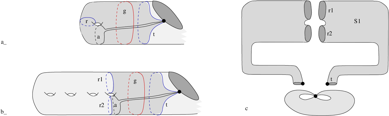
To prove (5.2), we cut the shaded area out of (by an arc and either a geodesic loop in case of genus or by two geodesics loops and in case of higher genus, see Fig. 5.4(a) and Fig. 5.4(b) respectively). Note that geodesic curves included in the relations (5.1) and (5.2) all lie inside the obtained area (since some representatives of the same isotopy class do lie there, and the boundary of is geodesic). We will build a new surface containing such that none of the curves participating in the equations will be separating on . Then we know from above that the value of will be equal to for all curves participating in (5.1) and (5.2), and so the formula (5.2) immediately follows from (5.1). Since the surface is embedded in isometrically, the same formula for lambda lengths holds for curves on , which implies that the value of is equal to as required.
To build the surface we proceed as on Fig. 5.4(c): we take two copies of , glue them together along the boundary components containing no marked points, then take a triangle with three vertices identified and attach free boundary components to two of the boundary components of the triangle. None of the curves contained in is separating in the constructed surface .
∎
5.4.2. Laurent polynomials for curves on orbifolds
Now we are ready to define the Laurent polynomials for curves on orbifolds in a given cluster.
For an arc or a pending arc the Laurent polynomial is the Laurent expansion of the cluster variable corresponding to .
Let be a (partial) unfolding of . Let be an arc or a pending arc. Let be a connected component of the lift of to . In view of Remark 4.2, coincides with the specialization of the Laurent polynomial . This motivates the following definition.
Definition 5.13 (Laurent polynomials for semi-closed loops).
Let be a semi-closed loop on , let be an unfolding of . Let be a connected component of the lift of to . Then define .
Remark 5.14.
The expression in Definition 5.13 depends on the choice of the unfolding of , however, the result does not depend on the unfolding. Indeed, by Lemma 5.12, the value of is the lambda length of , which implies that after the specialization of variables the function is equal to , where is the length of (independently on the choice of the unfolding ). Therefore, the value of depends on lambda lengths of arcs of a triangulation only, and thus does not depend on the unfolding .
By the same reason, the definition of does not depend on a connected component in the lift of .
The remark above motivates the following definition.
Definition 5.15.
The lambda length of a semi-closed loop is defined by , where is the length of .
Definition 5.16 (Laurent polynomials for closed curves).
Let be a closed curve on , let be an unfolding of such that lifts well in (it does exist by Lemma 4.7). Let be a connected component in the lift of to . Then define .
Remark 5.17.
Similarly to the case of semi-closed loops, the expression in the definition of the Laurent polynomial for a closed curve depends on the choice of the unfolding. However, due to the fact that the Laurent polynomial represents the lambda length of (see Lemma 5.12), represents the lambda length of . Hence, the definition of is independent on the choice of unfolding , neither it depends on the choice of the connected component in the lift of .
Remark 5.18.
Summarizing Definitions 5.13 and 5.16 we see that if a curve lifts well to an unfolding and is a connected component of the lift, then .
This natural property will be heavily used below.
Definition 5.19 (Laurent polynomials for multicurves and self-intersecting curves).
Let be a multicurve. Define .
For a formal sum of multicurves define .
Given a curve or a multicurve , define to be a complete resolution of all intersection points of . We consider as a formal sum of multicurves, each summand having non-self-intersecting components.
For a self-intersecting curve on define the Laurent polynomial as where is the complete resolution of all intersection points of .
Definition 5.20 (Constants for contractible curves).
If is a contractible curve then
- if is a closed contractible curve then ;
- if is a closed contractible curve around an orbifold point, then ;
- if is a contractible curve with both ends in an orbifold point then ;
5.5. Proof of skein relations on orbifolds
In this section we show the skein relations for the orbifold by proving the following theorem.
Theorem 5.22.
Let be a multicurve on an unpunctured orbifold . Let be an intersection point of (or a point of a self-intersection of some curve in ). Then , where is the resolution of at the intersection point as defined in Table 5.1.
To prove Theorem 5.22 we consider several cases. First, notice that if the point is a point of self-intersection of one curve , then there is nothing to prove (the statement holds by the definition of for a self-intersecting curve ). This holds for both regular and orbifold self-intersection points. So, we may assume that is an intersection point of two curves and . Clearly, it is sufficient to prove the theorem for the case . Now we are left with the following cases:
- 1.
- 2.
is an orbifold point, are are distinct thick curves. This case in considered in Lemma 5.25.
Lemma 5.23.
Let and be two curves intersecting at a regular point . Assume also that there exists an unfolding of such that each of the two curves and lifts well. Then .
In particular, this equation holds if at least one of and is not a closed curve.
Proof.
The statement follows from the definition of resolution .
More precisely, let be an unfolding of such that each of the two curves and lifts well. Let be any lift of , denote by and connected components of the lifts of and respectively containing . Then, according to Table 5.1, projects to (see also Remark 5.6). On the other hand, as skein relations hold on the surface . Since for each curve which lifts well, this implies .
Now, if none of and is a closed curve, then both and lift well in any unfolding, and we may apply the reasoning above. If is not a closed curve but is a closed curve, then by Lemma 4.7 there exists an unfolding where lifts well, so we can also apply the reasoning above.
∎
Lemma 5.24.
Let and be two curves intersecting at a regular point . Then .
Proof.
In view of Lemma 5.23 it is sufficient to prove the statement for the case when both and are closed curves.
It is easy to see that for every non-contractible closed curve on there exists an arc intersecting this curve. Let be an arc intersecting at some point ( may have more intersection points with and ). Since is an arc we may apply Lemma 5.23 to resolve the intersection and get , which implies
Note that as is an arc and is a closed curve, the resolution is a sum of two ordinary curves, so we can apply Lemma 5.23 to resolve the intersection and obtain
On the other hand, by Lemma 5.8 we have , which implies . Since is not a closed curve, we apply Lemma 5.23 to have
Summarizing the above computation, we obtain
Since the ring of Laurent polynomials has no zero divisors, this implies that which proves the lemma.
∎
Lemma 5.25.
Let and be two thick curves incident to the same orbifold point . Then .
Proof.
There are five possibilities for a pair of thick curves shown in Fig. 5.5 (depending on the types of thick curves and and the number of common vertices). In all of these cases the resolution contains no closed curves, which implies that all curves involved in as well as the curves and lift well in any unfolding . So, the required equation follows from the surface version of skein relations.
∎

In the case of principal coefficients, making use of Theorem 5.22, [MSW2, Propositions 6.4–6.6], and then specializing variables, we obtain the following relations.
Lemma 5.26.
where , , are monomials in variables computed in the following way:
where is equal to one half of the difference of the intersection numbers of the elementary lamination with and .
The intersection numbers of laminations with multicurves on orbifolds should be redefined as follows: every intersection of a lamination with a thick curve counts twice.
6. Bases , and on orbifolds
6.1. Definitions
Recall from [MSW2] that given a closed loop , the bangle is a union of loops isotopic to , and the bracelet is a closed curve obtained by concatenating exactly times (see Fig. 6.1). A band is defined in [T2] as an average of all possible end pairings of copies of , where is a short interval. In other words, can be considered as a weighted sum of unions of bangles and bracelets,
where is the set of all partitions of , and is the number of permutations in the symmetric group with given cyclic structure.

We define similar curves for a semi-closed curve as follows: if we denote by the closed curve which is a lift of in some degree two unfolding, then the lifts of and should coincide with and . Once bracelets are defined, we can define via the formula above.
More precisely, a bangle is a union of semi-closed loops isotopic to (see Fig. 6.2(a)). A bracelet is defined differently for odd and even . Denote by and the endpoints of . Then is a semi-closed curve with endpoints and going around and exactly times (see Fig. 6.2(b)). Finally, is a semi-closed curve with both endpoints being (or ) going around and exactly times (see Fig. 6.2(c)).
Note, that the equality still holds for semi-closed loops (since a closed loop around is isotopic to ).


The Laurent polynomials associated to bangles and bracelets can be computed via Definition 5.19. One can easily check that the obtained formulae coincide with ones for surfaces (see [MSW2, T2]): if is a semi-closed curve, then , and , where is the Chebyshev polynomial of the first kind defined by initial conditions , and recurrent relation , and is the Chebyshev polynomial of the second kind defined by initial conditions , and recurrent relation .
Following [MSW2], we define - and -compatibility.
Definition 6.1.
A finite collection of arcs, closed loops, pending arcs and semi-closed loops on is -compatible if no two elements of cross each other. The set of all -compatible collections in is denoted by .
A finite collection of arcs, pending arcs and bracelets is -compatible if
- •
no two curves intersect each other except for self-intersection of bracelets;
- •
given a closed loop or a semi-closed loop , there is at most one such that -th bracelet lies in . Moreover, there is at most one copy of this bracelet in .
The set of all -compatible collections in is denoted by .
After we extended the definition of - and -compatibility to the orbifold case, the definition of the bases and coincides with the one given in [MSW2] for the surface case:
Definition 6.2.
Given a curve , let be a Laurent polynomial defined in Section 5.4.2. Then
and
is called the bangle basis, and is called the bracelet basis.
Substituting bracelets by bands in the definition of -compatibility, we obtain the notion of -compatibility and the set of of all -compatible collections. The band basis is then defined as
6.2. Relations between , and
Similarly to the surface case, each element of the bracelet basis is an integer linear combination of elements of . More precisely, the only type of elements of not contained in is a bracelet and
where is a Chebyshev polynomial of the first kind (see above). Note that , where is a sum of smaller powers of , which implies that is an integer linear combination of , . In other words, each element of is an integer linear combination of elements of .
Exactly the same relation holds between and : each element of the band basis is an integer linear combination of elements of , and each element of is an integer linear combination of elements of . The reason is exactly the same: a Chebyshev polynomial of the second kind has the form , where is a sum of smaller powers of .
We will prove that is a basis for the cluster algebra , i.e. we will prove that
- elements of belong to the cluster algebra (Lemma 7.1);
- elements of span the cluster algebra (Lemma 7.2);
- elements of are linearly independent (Theorem 8.13).
Then all the statements for the sets and follow immediately from the fact that elements of and are related to elements of by a unitriangular integer linear transformation.
7. Skein relations and elements of
In this section, we show that elements of belong to cluster algebra and span it. We remind the reader that we consider cluster algebras originating from unpunctured orbifolds with at least two marked points at the boundary.
Lemma 7.1.
Elements of belong to the cluster algebra.
Proof.
We need to consider closed and semi-closed loops only. For closed loops, we apply [MSW2, Proposition 4.5] without any changes. For semi-closed loops we apply the same method as in the proof of [MSW2, Proposition 4.5], but we use skein relations for the configuration of curves shown in Fig. 7.1 on the left for the case when at least one boundary component of contains two or more marked points, and the configuration of curves shown in Fig. 7.1 on the right otherwise (one can see that Fig. 7.1 is a counterpart of [MSW2, Figure 11] and [MSW2, Figure 13]). After the resolution of all intersections, one of the summands will be a product of the Laurent polynomial associated to a closed loop around two orbifold points and boundary segments. Note that the former is equal to the Laurent polynomial associated to the semi-closed loop (as they have the same geodesic representative, cf. Remark 5.7 and Fig. 5.2(b)).
∎

Lemma 7.2.
is a spanning set for the cluster algebra.
Proof.
We need to show that every product of cluster variables can be represented as a sum of elements of .
Suppose that we have a collection of arcs and pending arcs . Consider a complete resolution of all intersection points of . We get a formal sum of multicurves, each consisting of mutually non-intersecting non-self-intersecting curves (i.e. we get a formal sum of collections of non-intersecting arcs, pending arcs, closed loops and semi-closed loops, and thus a formal sum of -compatible sets). Hence, is expressed as a sum of elements of .
∎
8. Linear independence of
In this section, we show that the set is linearly independent. Our proof follows the plan of the proof from [MSW2]. First, we show that a counterpart of [MSW2, Theorem 5.1] holds (Lemma 8.1), so we can make use of the notion of -vectors of elements of . Then we use tropical duality [NZ] and results of [MSW2] to associate -vectors of to certain laminations on the “reversed” associated orbifold (see Definition 8.3), which, in view of the results of [FeSTu3], implies bijection between -vectors of and elements of (Theorem 8.12). The application of [MSW2, Proposition 2.13] will complete the proof.
Lemma 8.1 (cf. [MSW2], Theorem 5.1).
Any element of contains a unique term not divisible by any coefficient variable, and the exponent vector of each other term is obtained from by adding a non-negative linear combination of columns of the extended exchange matrix .
Proof.
The proof follows from [MSW2, Theorem 5.1]. Let be an unfolding of . As we have already mentioned, every element of can be obtained from a corresponding element of by a specialization of variables, where is the bangle basis for the surface cluster algebra . This immediately implies the existence of the leading term (i.e., the term ) and defines -vectors for all elements of . The second statement of the lemma follows from the surface version and the definition of the unfolding of exchange matrix (see e.g. [FeSTu2]).
∎
Definition 8.2.
A -vector of an element of is the multidegree of its leading term .
Laminations and -vectors
First, we introduce reversed associated orbifold and its triangulation .
Definition 8.3.
Let be an associated orbifold with triangulation . The reversed associated orbifold is obtained from in the following way: replace all orbifold points by special marked points, and all the special marked points by orbifold ones. To obtain the corresponding triangulation from all pending arcs should be replaced by double ones, and the double arcs should be replaced by pending ones.
Remark 8.4.
If a triangulation on an associated orbifold is defined by a skew-symmetrizable matrix , then the triangulation on is defined by .
We will also need a notion of reversed elementary lamination on reversed associated orbifold .
Definition 8.5.
Given a triangulation of , a reversed elementary lamination is a lamination on with shear coordinates , where is located on -th place. Geometrically, is a “reflection” of the elementary lamination (w.r.t. ) in the th arc of .
According to [NZ, (1.13)], there is a duality between -vectors and -vectors of cluster algebras which can be expressed in the following terms:
where is the matrix composed of -vectors of a seed in the initial seed , and is the matrix composed of -vectors of a cluster in the initial cluster (see Section 2.2 for definitions). This duality holds in the assumptions of sign-coherence of -vectors, which is true for cluster algebras from orbifolds [FeSTu3, Theorem 14.1] (sign-coherence of -vectors in full generality was recently proved in [GHKK]).
Since the rows of -matrix are shear coordinates of elementary laminations (see [FeSTu3, Theorem 9.1]), and the (negative) transposed matrix corresponds to the reversed associated orbifold (see Remark 8.4), the duality can be reformulated in the following way.
Lemma 8.6.
Let be a triangulation of an associated orbifold corresponding to the initial cluster, and let be an arbitrary cluster variable (i.e., is some arc on ). Let be any triangulation of containing , and let be the corresponding elementary lamination with respect to . Then
Remark 8.7.
Comparing Lemma 8.6 with [MSW2, Corollary 6.15], we immediately obtain similar expression for closed loops on unpunctured surfaces.
Lemma 8.8.
Let be an unpunctured marked surface, and let be a triangulation of corresponding to the initial cluster. Let be the element corresponding to a closed loop on . Then
Here the closed loop is understood as a lamination consisting of a single curve.
Remark 8.9.
There is another way to prove Lemma 8.8 based on investigation of the band graph of closed loop (see [MW, MSW2]). More precisely, given a loop on , one can find an arc on which is very close to , see Fig. 8.1. It is easy to see that the vector of shear coordinates of can be obtained from the vector of shear coordinates of the reversed elementary lamination of by adding the vector . On the other hand, comparing the band graph of and the snake graph of , one can easily see that the monomials without coefficients (which correspond to the leading terms, and thus to -vectors) differ exactly by .
Notice that Fig. 8.1 represents an easy case when the curve intersects two arcs only (namely, and ) incident to its basepoint. In more general setting one uses the notion of fan introduced in [MSW2, Section 6.1]; this keeps the situation as simple as in the initial case and leads to exactly the same result.
The approach above seems to be suitable for generalizations to punctured case. For example, it allows an immediate generalization to punctured surfaces in the case of coming from ideal triangulation and having a conjugate pair in every puncture.

Since both -vectors and -vectors on orbifolds can be obtained via specialization of initial variables, and -vectors are exactly shear coordinates of elementary laminations, Lemma 8.8 gives rise to a similar statement for closed loops on associated orbifolds without punctures (and special marked points).
Lemma 8.10.
Let be an associated orbifold without punctures and special marked points, and let be a triangulation of corresponding to the initial cluster. Let be the element corresponding to a closed loop on . Then
Lemma 8.11.
The map assigning to an element of its -vector is surjective.
Proof.
Given any integer -vector , we find an element of with -vector .
Choose a triangulation of . As it is shown in [FeSTu3], there is a unique lamination on with shear coordinates (with respect to . As it is easy to see, every single curve of any lamination is either closed (or semi-closed) loop, or a reversed elementary lamination for some arc on (to obtain such just shift every boundary end of every curve clockwise till the closest boundary marked point).
Now construct a non-intersecting collection of curves on . It will consist of closed loops of (with semi-closed loops substituting loops around two special marked points in ), and all those arcs whose reversed elementary lamination is contained in . By Lemmas 8.6 and 8.10, the element of corresponding to the union of curves of has -vector .
∎
Theorem 8.12.
The map assigning to an element of its -vector is bijective.
Proof.
Consider first. We need to show that an element of with -vector is unique, the surjectivity follows from Lemma 8.11. Given an element of , we can define a lamination on in the following way. We keep all the closed (or semi-closed) curves of (with semi-closed curves substituted by loops around two special marked points), and take a reversed elementary lamination for every .
The considerations above show that the vector of shear coordinates of the lamination with respect to any triangulation is equal to negative -vector of with respect to . Moreover, two distinct elements of lead to two different laminations . According to [FeSTu3, Lemma 6.6], distinct laminations have distinct shear coordinates, which implies that two distinct elements of have distinct -vectors.
∎
Theorem 8.13.
The set is linearly independent.
9. Positivity of
Definition 9.1.
An additive basis of a -algebra is called positive if it has positive structure constants, i.e. for any one has with .
It was conjectured in [FG1] that both bases and for cluster algebras from surfaces are positive. However, it was demonstrated in [T1, Exercise 20.5, Lecture 18] that for the bangle basis the statement fails already in an annulus. More precisely, let and be marked points in different boundary components of the annulus and let be an arc connecting to and wrapping times, then it is easy to check that positivity fails for .
In [T2] D. Thurston proved positivity for the bracelet basis of the skein algebra of a surface (with punctures), which, in particular, implies positivity of the bracelet basis on an unpunctured surface. As a corollary, we get similar statement for an unpunctured orbifold.
Theorem 9.2.
The bracelet basis is positive.
The idea of proof in [T2] is to show that one can always resolve the crossings of a multicurve in such an order that negative terms (i.e. contractible loops) never arise.
We proceed as follows:
- 1)
use small deformations as in Fig. 5.2 to turn all thick curves into thin ones;
- 2)
substitute all orbifold points by punctures, so that we obtain a multicurve in a surface with punctures;
- 3)
resolve the intersections in such an order that no contractible loops will be obtained at any step;
- 4)
put the orbifold points back on their places;
- 5)
if needed, deform the closed loops around two orbifold points to semi-closed curves and arcs around one orbifold point to pending arcs.
The closed contractible curves will never arise, so that we obtain non-negative coefficients at each summand (see Remark 9.3).
Remark 9.3.
In the last line of Table 5.1 defining the resolution one can find . This does not prevent the bracelet basis from being positive. Indeed, the multicurve in this case contains a non-contractible thick curve (call it ) with two ends at the same orbifold point . Denote by and closed loops homotopic to the curves and (see Table 5.1). Then the skein relation becomes
so it also has non-negative coefficients.
10. Atomic bases for and finite type
Definition 10.1.
An element of a cluster algebra is positive if its Laurent expansion in every cluster has non-negative coefficients only, denote the set of positive elements by . An additive basis is atomic if if and only if can be written as a linear combination of with non-negative coefficients.
Cerulli Irelli [C2] proved that cluster monomials form an atomic basis of skew-symmetric cluster algebras of finite type. In [DT], Dupont and Thomas showed that the basis of a cluster algebra constructed by Dupont in [D2] is atomic. They also gave a similar proof for the case. Their atomic basis for coincides with the bracelet basis ( is represented by an annulus with and marked points on the boundaries). The cluster monomial basis of is also a particular case of the bracelet basis. In [GM], Gunawan and Musiker give a combinatorial proof of the fact the cluster monomial basis of the algebra of type is atomic.
Note that cluster algebras of classical finite and affine types originate from surfaces and orbifolds: can be realized as a disc with boundary marked points, as a disc with one special marked point and boundary marked points, as a disc with one orbifold point and boundary marked points, as a once punctured disc with boundary marked points, as an annulus with and marked points on the boundary components, and as a disc with two orbifold points and boundary marked points. In particular, is an unfolding of , is an unfolding of , and is an unfolding of . The aim of this section is to use unfoldings to adapt the proof from [DT] to the orbifold case. Furthermore, it was shown in [FeSTu2] that a cluster algebra of type also can be unfolded to a cluster algebra of type . As an application of our methods, we extend the result of [C2] to the skew-symmetrizable case.
It was shown in [MSW1, MSW2] that cluster variables and bracelets on an unpunctured surface are positive. Using unfolding, we can see that cluster variables and bracelets on an unpunctured orbifold are also positive (cluster variables on any orbifold are positive by [FeSTu3, Theorem 13.1]). This immediately implies that all elements of are positive, and thus any linear combination of elements of with non-negative coefficients is positive.
The goal of this section is to prove the following theorems.
Theorem 10.2.
Cluster monomial bases of skew-symmetrizable cluster algebras of finite type are atomic.
Theorem 10.3.
The bracelet basis on the disc with two orbifold points and marked points is the atomic basis of the cluster algebra of affine type .
First, let be the cluster monomial basis of a skew-symmetric cluster algebra of finite type. Let be any cluster. Take any cluster variable , and take any cluster monomial containing as a factor. Consider the Laurent expansion of in the cluster (we will call it -expansion of ). Following [CL], we say that a term of the -expansion of is a proper Laurent monomial if it has negative degree with respect to at least one variable, and the cluster algebra has the proper Laurent monomial property if for any two clusters and of , every monomial in in which at least one factor does not belong to is a linear combination of proper Laurent monomials in .
Lemma 10.4 ([CKLP], Corollary 3.4).
Any skew-symmetric cluster algebra has the proper Laurent monomial property.
Now consider any element , where are cluster monomials. Choose any . Let be a cluster containing all the cluster variables that are factors of . Clearly, the -expansion of is just a monomial. Thus, the following lemma is an immediate corollary of Lemma 10.4.
If we know that is positive, Lemma 10.5 implies that coefficient of in the expression for is non-negative, which implies that is an atomic basis (as was arbitrary).
We are now ready to prove the first theorem. The proof for algebras of type and can be formulated in terms of triangulations, and the proof for algebra can be formulated in terms of triangulated heptagons [Lam], but we avoid this language to produce a uniform reasoning (algebra of type has rank two and its cluster monomial basis was studied in [SZ, LLZ]).
Proof of Theorem 10.2.
The basis for the corresponding cluster algebra consists of cluster monomials only. To prove the theorem, we need to show that the skew-symmetrizable counterpart of Lemma 10.5 holds. Namely, we want to prove that a Laurent expansion of a cluster monomial does not have other summands being cluster monomials. As in the skew-symmetric case, this proves the atomicity of the basis .
We prove the counterpart of Lemma 10.5 by contradiction. Suppose it fails, so there exist a cluster of , a cluster monomial in , and a cluster monomial containing at least one variable not compatible with factors of such that the -expansion of contains a term .
Consider an unfolding of , and denote by the cluster of which gives after the specialization of variables. By the construction of the unfolding, cluster monomials lift to cluster monomials with literally the same expansions (after identifications of the corresponding variables). Thus, the -expansion of some lift of contains (after the specialization of variables) the term . Our goal is to show that this contradicts Lemma 10.4.
Let be cluster variables of , and denote the lifts of (some of have only one lift, we will denote these by ). Denote by the factors of , and by the lifts of (again, we will denote by those who are the unique lifts).
Denote by any lift of (note that is a cluster monomial of ). Take the term in the -expansion of which becomes after specialization of variables, this term should have the form
where is the index set of variables of with a unique lift, , , and .
Now consider another lift of the cluster monomial obtained from in the following way: for every factor we swap all the lifts and . Then we obtain a cluster monomial of compatible with , and its -expansion can be obtained from the -expansion of by swapping all the and (this can be easily seen for individual cluster variables and by, e.g., using cluster automorphisms technique [Law], and thus holds for cluster monomials as well). Therefore, the -expansion of has a term
Since and are cluster monomials in the same cluster of , their product is also a cluster monomial, and its -expansion contains the product of the two terms above, which is not a proper Laurent monomial since . This contradicts Lemma 10.4.
∎
For the case the situation is a bit more involved. Let be the bracelet basis of a cluster algebra of type , take an element , where . Choose any . Let be any triangulation of an annulus containing all the arcs from the multicurve (note that may also contain a bracelet). Now consider the -expansions of all .
This time is either a monomial in these variables (if contained arcs only), or a sum of Laurent monomials with positive coefficients (if contains a bracelet). In the latter case, there are infinitely many triangulations containing all the arcs from the multicurve .
Lemma 10.6 ([DT]).
(i) If is not compatible with , and contains no bracelets, then the -expansion of is a proper Laurent monomial. In particular, the -expansion of does not contain any term coinciding with .
(ii) Let contain a bracelet. If , then there exist a sequence of triangulations such that each contains all arcs of , , and a term of -expansion of such that for any the -expansion of does not contain .
We will recall the construction of and during the proof.
As in the finite type case, Lemma 10.6 implies that is an atomic basis.
Proof of Theorem 10.3.
Similarly to the proof of Theorem 10.2, we now need a counterpart of Lemma 10.6 to hold. The corresponding orbifold is a disc with two orbifold points and marked points, the bracelet basis for the corresponding cluster algebra contains cluster monomials and one family of bracelets. If we take a double cover of the disc branching in orbifold points only, we obtain an annulus with marked points on each boundary component, so that the unfolding is . Let be an element of the basis .
If does not contain bracelets, then the argument is similar to one for . Take any basis element and any triangulation containing all the arcs of . Let be the set of all arcs in , and let be the lifts of (the two pending arcs of have only one lift each). Choose any lift of , take any term of -expansion of . By Lemma 10.6(i), this term has negative degrees with respect to some and . If we assume that after identification of and the term will coincide with then it should become a monomial, which implies that every degree of with respect to and have to be positive and greater or equal to the moduli of the corresponding negative ones. Assume that this is the case.
First, assume that is a cluster monomial. Then we can consider the multicurve symmetric to , i.e. we substitute all the entries of by and vice versa for every . Note that is compatible with , and thus, we can consider a cluster monomial and the term of its -expansion obtained as the product of and , where is the term symmetric to . By the assumption, the term of the -expansion of this monomial will have positive degree with respect to any variable, which contradicts Lemma 10.6(i).
Now, assume that contains a bracelet , where is the semi-closed loop joining two orbifold points. Then contains a bracelet . Note that every term of the -expansion of can be considered as some term of the -expansion of . Thus, we can also consider : although it is not an element of the bracelet basis of , all the terms of its -expansion are terms of the -expansion of an element of the bracelet basis obtained from by dividing by and multiplying by . Considering the same term as in the previous case, we see that it has positive degree with respect to any variable, which contradicts Lemma 10.6(i).
Assume now that consists of a bracelet and a collection of arcs . Following [DT], define triangulations containing all the arcs of as follows. There exists a marked point (call it ) which can be joined with both orbifold points without intersecting arcs of . Add to arcs of two shortest pending arcs ending at and an arc with both ends at , then extend this to any triangulation, this will be . To obtain , apply a half of the Dehn twist to the loop around two orbifold points times. Denote the pending arcs by and . An easy computation shows that the -expansion of has a term (see also [DT]). Consider the term of the -expansion of . The lifts and on the annulus are exactly the triangulation and the term used in Lemma 10.6(ii), see [DT]. We now want to show that given , for large enough no term of the -expansion of coincides with . Since any element of cluster algebra is a finite linear combination of elements of , this will complete the proof.
We proceed in exactly the same way as in the previous case. Take any lift of and assume that some term of the -expansion of coincides with after specialization of variables. As before, consider the multicurve symmetric to and the corresponding term of , take the product of these two terms: the result is a term of the -expansion of an element of the bracelet basis of obtained from by dividing by and multiplying by . By the assumption, this will have a form for some lift of . Thus, we see that -expansion of some element of the bracelet basis of contains a term coinciding with , where . According to Lemma 10.6(ii), this cannot hold for large enough. This completes the proof of the theorem.
∎
References
- [CK] P. Caldero, B. Keller, From triangulated categories to cluster algebras, Invent. Math. 172 (2008), 169–211.
- [CLS] I. Canakci, K. Lee, R. Schiffler, On cluster algebras from unpunctured surfaces with one marked point, Proc. Amer. Math. Soc. Ser. B 2 (2015), 35–49.
- [CT] I. Canakci, P. Tumarkin, Bases of cluster algebras from unpunctured orbifolds with one marked point, in preparation.
- [C1] G. Cerulli Irelli, Cluster algebras of type , Algebr. Represent. Theory 15 (2012), 977–1021.
- [C2] G. Cerulli Irelli, Positivity in skew-symmetric cluster algebras of finite type, arXiv:1102.3050.
- [CE] G. Cerulli Irelli, F. Esposito, Geometry of quiver Grassmannians of Kronecker type and applications to cluster algebras, Algebra Number Theory 5 (2011), 777–801.
- [CKLP] G. Cerulli Irelli, B. Keller, D. Labardini-Fragoso, P.-G. Plamondon, Linear independence of cluster monomials for skew-symmetric cluster algebras, Compos. Math. 149 (2013), 1753–1764.
- [CL] G. Cerulli Irelli, D. Labardini-Fragoso, Quivers with potentials associated to triangulated surfaces, part III: Tagged triangulations and cluster monomials, Compos. Math. 148 (2012), 1833–1866.
- [Ch] L. Chekhov, Orbifold Riemann surfaces and geodesic algebras, J. Phys. A: Math. Theor. 42 (2009), 304007, 32 pp.
- [ChM] L. Chekhov, M. Mazzocco, Orbifold Riemann surfaces: Teichmüller spaces and algebras of geodesic functions, Russian Math. Surveys 64 (2009), 1079–1130.
- [CGMMRSW] M. W. Cheung, M. Gross, G. Muller, G. Musiker, D. Rupel, S. Stella, H. Williams, The greedy basis equals the theta basis, J. Combin. Theory A, 145 (2017), 150–171.
- [DXX] M. Ding, J. Xiao, F. Xu, Integral bases of cluster algebras and representations of tame quivers, Algebr. Represent. Theory 16 (2013), 491–525.
- [D1] G. Dupont, Generic variables in acyclic cluster algebras and bases in affine cluster algebras, arXiv:0811.2909.
- [D2] G. Dupont, Transverse quiver Grassmannians and bases in affine cluster algebras, Algebra Number Theory 4 (2010), 599–624.
- [D3] G. Dupont, Generic variables in acyclic cluster algebras, J. Pure Appl. Algebra 215 (2011), 628–641.
- [DT] G. Dupont, H. Thomas, Atomic bases in cluster algebras of types and , Proc. London Math. Soc. 107 (2013), 825–850.
- [FeSTu1] A. Felikson, M. Shapiro, P. Tumarkin, Skew-symmetric cluster algebras of finite mutation type, J. Eur. Math. Soc. 14 (2012), 1135–1180.
- [FeSTu2] A. Felikson, M. Shapiro, P. Tumarkin, Cluster algebras of finite mutation type via unfoldings, Int. Math. Res. Notices (2012), 1768–1804.
- [FeSTu3] A. Felikson, M. Shapiro, P. Tumarkin, Cluster algebras and triangulated orbifolds, Adv. Math. 231 (2012), 2953–3002.
- [FG1] V. Fock, A. Goncharov, Moduli spaces of local systems and higher Teichmüller theory, Publ. Math. Inst. Hautes Études Sci. 103 (2006), 1–211.
- [FG2] V. Fock, A. Goncharov, Dual Teichmüller and lamination spaces. Handbook of Teichmüller theory. Vol. I, 647–684, IRMA Lect. Math. Theor. Phys., 11, Eur.Math. Soc., Zürich, 2007.
- [FG3] V. Fock, A. Goncharov, Cluster ensembles, quantization and the dilogarithm, Ann. Sci. Éc. Norm. Supér. 42 (2009), 865–930.
- [FST] S. Fomin, M. Shapiro, D. Thurston, Cluster algebras and triangulated surfaces. Part I: Cluster complexes, Acta Math. 201 (2008), 83–146.
- [FT] S. Fomin, D. Thurston, Cluster algebras and triangulated surfaces. Part II: Lambda lengths, arXiv:1210.5569.
- [FZ1] S. Fomin, A. Zelevinsky, Cluster algebras I: Foundations, J. Amer. Math. Soc. 15 (2002), 497–529.
- [FZ2] S. Fomin, A. Zelevinsky, Cluster algebras IV: Coefficients, Compos. Math. 143 (2007), 112–164.
- [GHKK] M. Gross, P. Hacking, S. Keel, M. Kontsevich, Canonical bases for cluster algebras, arXiv:1411.1394
- [GLS] C. Geiss, B. Leclerc, J. Schröer, Generic bases for cluster algebras and the Chamber Ansatz, J. Amer. Math. Soc. 25 (2012), 21–76.
- [GM] E. Gunawan, G. Musiker, -path formula and atomic bases for cluster algebras of type , SIGMA 11 (2015), 060, 46pp.
- [K] M. Kashiwara, Bases cristallines, C. R. Acad. Sci. Paris Sér. I Math. 311 (1990), 277–280.
- [Lam] L. Lamberti, Combinatorial model for the cluster categories of type , J. Alg. Combin. 41 (2015), 1023–1054.
- [Law] J. Lawson, Cluster automorphisms and the marked exchange graphs of skew-symmetrizable cluster algebras, Electron. J. Combin. 23 (2016), Paper #P4.41.
- [LLZ] K. Lee, L. Li, A. Zelevinsky, Greedy elements in rank cluster algebras, Selecta Math. 20 (2014), 57–82.
- [L] G. Lusztig, Canonical bases arising from quantized enveloping algebras, J. Amer. Math. Soc. 3 (1990), 447–498.
- [MSW1] G. Musiker, R. Schiffler, L. Williams, Positivity for cluster algebras from surfaces, Adv. Math. 227 (2011), 2241–2308.
- [MSW2] G. Musiker, R. Schiffler, L. Williams, Bases for cluster algebras form surfaces, Compos. Math 149, 2, (2013) 217-263.
- [MW] G. Musiker, L. Williams, Matrix Formulae and skein relations for cluster algebras from surfaces, Int. Math. Res. Notices (2013), 2891–2944.
- [NZ] T. Nakanishi, A. Zelevinsky, On tropical dualities in cluster algebras, Contemp. Math. 565 (2012) 217–226
- [P] R. C. Penner, The decorated Teichmüller space of punctured surfaces, Comm. Math. Phys. 113 (1987), 299–339.
- [Pl] P. G. Plamondon, Generic bases for cluster algebras from the cluster category, Int. Math. Res. Notices (2013), 2368–2420.
- [SZ] P. Sherman, A. Zelevinsky, Positivity and canonical bases in rank cluster algebras of finite and affine types, Mosc. Math. J. 4 (2004), 947–974.
- [T1] D. Thurston, The Geometry and Algebra of Curves on Surfaces, Lecture course in UC Berkeley, 2012. Notes by Qiaochu Yuan http://math.berkeley.edu/~qchu/Notes/274/
- [T2] D. Thurston, Positive basis for surface skein algebras, Proc. Natl. Acad. Sci. USA 111 (2014), 9725–9732.
- [T] W. P. Thurston, On the geometry and dynamics of diffeomorphisms of surfaces, Bull. Amer. Math. Soc. (N.S.) 19 (1988), 417–431.