On the Evolution of Jet Energy and Opening Angle in Strongly Coupled Plasma
Abstract
We calculate how the energy and the opening angle of jets in SYM theory evolve as they propagate through the strongly coupled plasma of that theory. We define the rate of energy loss and the jet opening angle in a straightforward fashion directly in the gauge theory before calculating both holographically, in the dual gravitational description. In this way, we rederive the previously known result for without the need to introduce a finite slab of plasma. We obtain a striking relationship between the initial opening angle of the jet, which is to say the opening angle that it would have had if it had found itself in vacuum instead of in plasma, and the thermalization distance of the jet. Via this relationship, we show that SYM jets with any initial energy that have the same initial opening angle and the same trajectory through the plasma experience the same fractional energy loss. We also provide an expansion that describes how the opening angle of the SYM jets increases slowly as they lose energy, over the fraction of their lifetime when their fractional energy loss is not yet large. We close by looking ahead toward potential qualitative lessons from our results for QCD jets produced in heavy collisions and propagating through quark-gluon plasma.
Keywords
gauge-gravity correspondence, quark-gluon plasma, jets, heavy ion collisions1 Introduction and summary of results
Consider a light quark jet moving through an infinite volume of static strongly coupled plasma with temperature . Broadly speaking, the jet consists of an energetic spray of excitations localized within a narrow cone of opening angle about the axis of propagation of the jet. As the jet propagates though the plasma, energy and momentum leave the jet and excite hydrodynamic modes in the plasma. The excited hydrodynamic modes then transport the lost energy and momentum away from the jet. Interesting questions to consider include: what is the rate at which the jet loses energy to the plasma? How does change as the jet propagates? How far can the jet travel before it thermalizes? How do the rate of energy loss and the thermalization distance depend on initial conditions, including in particular the initial energy of the jet and the initial value of ?
Holographic duality [1, 2, 3] relates the dynamics of the strongly coupled plasma in certain large gauge theories to the dynamics of classical black holes in one higher dimension. The simplest theory with a dual gravitational description is 3+1-dimensional supersymmetric Yang-Mills theory (SYM), whose dual description is that of gravity in an asymptotically AdS5 spacetime. Thanks to this dual classical gravity description, the properties of SYM plasma are under much better theoretical control than is the case for QCD plasma. This has motivated much interest in using SYM plasma as a toy model for the formation, properties, and dynamics of real quark-gluon plasma and the dynamics of probes therein. (For reviews, see for example Refs. [4, 5, 6, 7, 8].)
Models for jet quenching in the strongly coupled plasma of SYM theory have been studied extensively. (See, for example, Refs. [9, 10, 11, 12, 13, 14, 15, 16, 17, 18, 19, 20, 21, 22, 23, 24, 25, 26, 27, 28, 29, 30, 31, 32, 33].) On first hearing this sounds surprising since, unlike in QCD, in SYM theory hard processes with large momentum transfer do not produce jets [34, 35]. Nevertheless, one can construct states in SYM theory which have highly energetic and localized excitations — which we shall call “jets” — which propagate arbitrarily far through plasma before thermalizing. Indeed, over the past decade, different authors [9, 10, 12, 17, 36, 19, 20, 21, 22, 23, 25, 26, 27, 28, 30] have introduced different ways of constructing states in SYM theory with “jets.” However, thus far most authors have defined physical quantities, such as the “jet” energy loss rate, via gravitational quantities instead of directly in terms of field theoretic variables. Together with the differing models for “jets,” this has led to different authors predicting qualitatively different energy loss rates [24]. Our strategy is to work the other way around. We use the gravitational description to compute the expectation value of the SYM stress tensor, , and extract physical quantities, including the rate of energy loss and the evolution of the opening angle, directly from .
In this paper, we shall study the “jets” introduced in Refs. [36, 19] and analyzed further in Ref. [30] which consist of massless quark jets represented in the dual gravitational description as arcs of rapidly moving, falling, open strings. We consider the propagation of these “jets” in an infinite volume of strongly coupled plasma, dispensing with the finite slab of plasma introduced as a device in Ref. [30]. There are (at least) two ways to use results about how “jets” lose energy to gain insights into jet quenching in QCD. One option is to take the form for the “jet” energy loss rate and apply it parton-by-parton to every parton in a QCD jet, letting QCD describe the production of a hard parton and its subsequent fragmentation into a shower, and using the SYM “jet” energy loss rate to describe how each parton in the shower loses energy. This yields the hybrid model for jet quenching introduced in Refs. [31, 33]. These authors have shown that this approach provides a good representation of much existing jet data, and have used it to make predictions for many experimental measurements soon to come. The second possible path toward insights about jet quenching in QCD is more radical: one can think of the “jets” that we analyze literally as proxies for QCD jets, and look for insights from our calculation into how jets change in shape, as well as lose energy, as they propagate through strongly coupled plasma. We shall take some steps in this second direction in Section 4. For this reason, and for simplicity, we shall henceforth refer to our “jets” just as jets.
We focus on jets that have vanishingly small size at the moment when they are produced. In the dual gravitational description, this requires considering strings that are created at a point asymptotically close to the AdS boundary. The jets we study initially expand linearly in time as they propagate, meaning that initially they expand with a constant opening angle . If the jets were in fact in vacuum, would remain constant at its initial value . For the jets we consider, though, as they propagate their opening angle increases as they lose energy and excite hydrodynamic modes of the plasma. If the volume of plasma in which they are propagating is large enough, eventually after traveling a distance they have lost all of their initial energy and they thermalize. We shall see that is determined by . In any consideration of high energy jets produced in heavy ion collisions, the plasma will end before the jet thermalizes, meaning that jets emerge from it rather than thermalizing in it. We shall see, though, that the thermalization distance plays a central role throughout our calculations, including in the expressions we obtain that describe how the energy and opening angle of jets that travel only a fraction of evolve.
In order to crisply separate the jet from the plasma and thereby systematically define the properties of the jet, including its rate of energy loss and its opening angle, it is useful to focus on states where there is a large separation of scales. Indeed, as is the characteristic microscopic scale in strongly coupled plasma, it makes no sense to attempt to define instantaneous properties of a jet with any spatial or temporal fidelity smaller than ! With this in mind, we study jets whose and focus on physics in the region
| (1) |
which we shall refer to as the “steady-state region” (SSR). Jets whose have high initial energy where is the (large) ’t Hooft coupling of the strongly coupled gauge theory [19, 17]. The SSR becomes arbitrarily close to 100% of the jet’s trajectory as , since the SSR includes any such that tends to a constant between 0 and 1 in this limit. In the SSR, as the jet moves over distances with , the evolution of the jet is steady-state, with deviations from steady-state behavior suppressed by powers of . This allows for simple definitions of both the instantaneous rate of energy loss and the instantaneous opening angle in terms of , definitions which we give below in Sec. 2. As we shall see below, as and the jet exits the SSR, the energy loss rate and opening angle grow rapidly, the separation between the jet and plasma becomes less and less distinct, and the jet’s instantaneous energy loss rate and opening angle become less and less crisply defined.
We now summarize our principal results.
We find that jets with thermalization distance have initial opening angles
| (2) |
where is the initial jet energy, is an energy scale that depends on how the jet is prepared, and is an pure number. We shall discuss each of these three quantities in turn.
The initial jet energy in (2) is the energy when the jet enters the SSR. It does not make sense to define the jet energy until some time after its creation, as at its creation gluon fields around its creation event are created and we need to wait for the jet to separate from gluon fields that are not part of the jet before defining the energy of the jet. This is equally true in vacuum or in plasma, and it is somewhat analogous to what is described by soft functions in jet production calculations in QCD. In the strongly coupled plasma, the gluonic energy that is not co-moving with the jet thermalizes within a time of order , after which the initial jet energy can be crisply defined. The constant is a temperature-independent energy scale proportional to with a temperature-dependent minimum value proportional to , meaning that must be large compared to . is small compared to so . The value of depends on details of how the state is prepared. The constant appearing in (2) depends on the precise definition of the jet opening angle, but once this is defined, is the same for every jet. We shall define precisely in Sec. 2, but it is in essence the half-width-at-half-maximum of the jet, meaning that the flux of energy an angle away from the jet axis is half as large as the flux along the jet axis. With our definition of , we find . (If, for example, we had instead defined as the angle at which the energy flux is 10% of its maximum value on the jet axis, would be larger by a factor of 2.23507 and the angular size each of our jets, defined in this alternate fashion, would be larger by this factor than is the case with the definition we have chosen.)
Likewise, the thermalization distance reads [19, 17]
| (3) |
for the same . Therefore, among the jets with some given initial energy , the jets that have the maximum possible the thermalization distance (i.e. have the minimum possible value of ) have a minimal but nonzero opening angle. To make contact with notation introduced in previous literature, we can introduce the dimensionless constant via , so that Eq. (3) takes the form . The maximum value of , corresponding to the minimum value of , has been estimated to be around 0.5 to 1 [19, 27]. We see from (2) that the fact that has a minimum value means that, for a given , the initial opening angle has a nonzero minimum value. Equivalently, it means that the range of possible values of for jets with a given has a nonzero minimum value.
Using (2), can be eliminated from (3) to yield
| (4) |
We therefore see that the thermalization distance is entirely determined by the initial opening angle of the jet and the temperature of the plasma; it is independent of the details of how the jet is prepared that are encoded in .11 1 This independence of the thermalization distance on extraneous details is obtained for jets that have zero size when they are produced and that initially behave as if they were produced in vacuum. We are considering only such jets. They expand with an opening angle that is initially , as if in vacuum, and subsequently increases due to the presence of the plasma, as we shall see below. If, as in Refs. [27, 28], one instead considers jets produced with a nonzero initial size, the relation (4) need not be valid. For example, it is possible (although doing so takes a long time in the past, arranging the shape of the trailing string) to prepare ‘initial’ states with nonzero size that have but have a finite [27, 28]. This is a remarkable result, as it says that all jets with a given initial opening angle , with any value of the initial energy above the minimum possible, have the same thermalization distance.
We find that in the SSR the jet’s instantaneous opening angle increases steadily as the jet propagates through the strongly coupled plasma and is well-approximated by
| (5) |
with the inverse of
| (6) |
with the Gauss Hypergeometric function. The approximation (5) describes the full result obtained in Sec. 3.2 to within 1.5%. In the left panel of Fig. 1, we plot the approximation (5) for . We see from Fig. 1 that the opening angle increases only very slowly until . Indeed, at small we can expand Eq. (5), obtaining
| (7) |
with the constant
| (8) |
In any consideration of jets in heavy ion collisions which travel through a length of plasma that is much less than , the expansion (7) is the form of our result for the evolution of the jet opening angle that is of interest. We can, however, use the approximation (5) at larger values of . It is easy to see from (5) that as the opening angle grows like
| (9) |
From this expression and (4), we see that as increases to — where the jet exits the SSR — the opening angle of the jet increases rapidly to . At this point neither our result (5), plotted in the left panel of Fig. 1, nor the expression (9) are valid any longer. In fact, once the jet is itself no longer sharply defined.
We also calculate the instantaneous rate of energy loss for the jet while it is in the SSR and find
| (10) |
This expression is identical to that obtained in our previous work [30]. From Eqs. (4) and (10) we therefore see that the energy loss rate is, up to normalization, entirely fixed by the opening angle of the jet and the plasma temperature. In particular, the fractional energy loss suffered by a jet propagating for a distance , obtained by integrating (10), is entirely determined by , and in the single combination and doesn’t depend on at all. All jets with a given initial opening angle , with any value of the initial energy above the minimum possible, suffer the same fractional energy loss if they traverse the same length of plasma. In this sense, jet energy loss is controlled by the initial opening angle of the jet and the trajectory of the jet through the plasma, not by the initial energy of the jet.
In the right panel of Fig. 1 we plot . Mirroring the behavior of above, the jet energy decreases only slowly until . Indeed initially, meaning that very little energy is lost. In this regime we can expand and integrate (10), obtaining
| (11) |
This expansion, to the order shown, deviates from the full result for obtained by integrating (10) by 0.2% at and only by 2.5% for , which is to say by at most 2.5% over distances for which . However, as , diverges like , meaning that the majority of the jet’s energy is lost in the final stages of its trajectory. In fact, more than three quarters of the initial energy of the jet is lost in the last quarter of and the last of the jet’s energy is lost in the last of its trajectory. The rate of energy loss increases until , at which point the jet exits the SSR and the jet’s instantaneous rate of energy loss becomes ill-defined. Nevertheless, we see from (10) and (3) that for , the jet still has a parametrically large amount of energy (compared to ), meaning that the thermalization of the jet coincides with a dramatic burst of energy being transferred to the plasma. This behavior, which was first suggested in [19], is reminiscent of a Bragg peak.
After setting up our calculation in Section 2 in the gauge theory, and obtaining all the results above in Section 3 via holographic calculations, in Section 4 we shall close with some speculations about the qualitative lessons for real jets, produced in heavy ion collisions, that may be learned from the results that we have summarized here.
We defer to an Appendix a discussion of why the ratio of the initial jet mass to the initial jet energy is not a proxy for the initial jet angle of the jets that we study, showing there that in the limit. This happens because these jets have stress energy flowing at angles considerably larger than when is small, and these large-angle (maybe better to say not-small-angle) tails of the jets contribute to in a way that they do not contribute to the jet opening angle itself.
2 Defining the opening angle and energy loss rate in the field theory
Consider a jet produced at and propagating in the -direction through an infinite and static plasma at temperature . Fig. 2 shows a far-zone cartoon of the jet at some fixed time. The jet consists of a localized distribution of energy, within the red oval in Fig. 2, propagating in the -direction whilst losing energy and momentum to the plasma. The lost energy and momentum excite hydrodynamic modes in the plasma which in turn transport the lost energy and momentum away from the jet. In an infinite plasma, the jet propagates a distance before it has lost all of its energy and momentum and thermalized. To have a well-defined jet and correspondingly, to crisply define the local energy loss rate and opening angle , it is necessary to consider jets whose is much greater than the plasma’s characteristic microscopic scale, which at strong coupling is . Indeed, the scaling relation (3) means this limit is realized by taking the initial jet energy , with the ’t Hooft coupling of the gauge theory. When both the rate of energy loss and the opening angle must be slowly varying functions of , changing substantially only over scales of order . In other words, over scales , the evolution of the jet must be approximately steady-state with deviations from steady-state behavior suppressed by powers of . Our calculations presented below show this remains true as long as lies in the SSR, Eq. (1) above. We shall obtain expressions for and within the domain (1).
Before proceeding, it is worth noting that although we shall derive results valid throughout the range (1), in drawing qualitative conclusions from our results about the behavior of high energy jets in heavy ion collisions the full range is not relevant. The highest energy jets that are observed in heavy ion collisions are, by definition, those that have emerged from the droplet of plasma created in the collision long before they travel a distance .
Let us begin by defining the opening angle. Fig. 3 shows a cartoon of the jet at some fixed time. The jet consists of a thin shell of energy propagating in the -direction whilst expanding in the transverse directions. In the past and future the jet was and will be located in the yellow shaded region in the figure, which is bounded by some transverse envelope function . The slope of the tangent line to the envelope function, shown as the dashed purple line in the figure, defines the opening angle of the jet,
| (12) |
If the jet were in vacuum, would be constant, meaning that the yellow shaded region would be bounded by a straight line like the dashed purple line. We can now be more precise about what we mean by the phrase “steady-state”. In the steady-state region (1), if we follow the jet only over some length scale its opening angle does not change much, meaning that as it propagates over the distance its transverse extent grows approximately linearly, as if in vacuum. The effects of the presence of the plasma accumulate over longer distances, as grows and the boundary of the yellow shaded region curves outward.
To turn the picture in Fig. 3 into a calculation of , we need a definition of the transverse envelope function . A simple definition of comes from considering the flux of energy through a surface at some constant ,
| (13) |
The maximum of , which occurs at , must grow as the jet energy is taken higher and higher and correspondingly, as is taken larger and larger. We choose to define the transverse envelope by the half width at half maximum of ,
| (14) |
As we shall see below in Sec. 3.2, in the SSR (1) we have , with growing to order only when .
We now turn to the definition of the rate of energy loss. As we have done for the jet opening angle, we wish to define the rate of energy loss in the field theory, without introducing the dual gravitational description. A simple procedure to compute the energy loss rate is to surround the jet (the red oval in Fig. 2) by a sphere and to compute the flux of energy through ,
| (15) |
The sphere is depicted as the yellow dashed circle in the cartoon shown in Fig. 2. It has a constant radius and is centered on the center of the jet at the time shown. How big should be? Since in the SSR the size of the jet is , a natural choice is . With this choice, the non-hydrodynamic physics of the jet itself, found within the red oval in Fig. 2, lies well inside the sphere at all times meaning that at all times the physics on the surface is described well by hydrodynamics and the rate of energy loss (15) is simply the rate at which energy flows into hydrodynamic modes. However, it should be emphasized that in the SSR, the precise size of doesn’t matter as long as since the jet evolution is steady-state over scales .
We shall compute the rate (15) at which energy flows into hydrodynamic modes in Fourier space. Consider the Fourier transform
| (16) |
and focus on slowly varying long wavelength modes with and fixed in the large limit. In this limit, the stress must take the form
| (17) |
where satisfies the constitutive relations of hydrodynamics and describes the nonhydrodynamic contribution to the stress tensor. Upon Fourier transforming back to real space, must have a gradient expansion in terms of derivatives of delta functions centered on the center-of-mass of the jet,
| (18) |
In other words, at low frequencies encodes the long wavelength limit of the localized stress near the jet. Moreover, the total stress is conserved so
| (19) |
meaning sources the hydrodynamic flow. At low frequencies, the Fourier transform of the jet energy, , must be given by .
What are the expected forms of and ? In the large limit salient to holography, the response of the plasma to the presence of the jet is suppressed and the constitutive relations of linear hydrodynamics yield the leading order long wavelength expansion
| (20) | ||||
where and are the proper energy and pressure, respectively, with and their equilibrium values, and is the fluid velocity. Conformal invariance in SYM requires to be traceless, which means .
Likewise, at small momentum the tensor structure of can only depend on the velocity of the jet’s center of mass, , and on the metric tensor . Demanding tracelessness then requires . However, for a jet composed of massless excitations, the velocity of the jet’s center of mass is related to the jet’s opening angle such that for jets whose , meaning the center of mass of a well collimated jet moves at approximately the speed of light. More specifically, we shall show in Appendix A that
| (21) |
As , in the limit we must simply have
| (22) |
Note that only depends on the combination because the jet center of mass trajectory, , translates uniformly.
We therefore conclude that by computing the long wavelength limit of , and then matching onto the expected forms (17), (20) and (22), the low frequency limit of the jet energy can be obtained. More precisely, the real space function obtained in this manner is the derivative expansion of the energy loss in (15). Nevertheless, in the limit, where the dynamics are approximately steady state, the two procedures for obtaining the energy loss rate must agree.
As a matter of convenience, we will find it useful to extract by projecting onto the traverse traceless mode of . Let , denote polarization vectors orthogonal to . Define the transverse traceless mode of the stress,
| (23) |
The hydrodynamic stress in (20) lacks a transverse traceless mode, so . Substituting (22) into (23), we conclude that in the long wavelength limit, the transverse traceless mode must read
| (24) |
Our strategy for computing the opening angle and energy loss in holography is therefore to construct states where . For the opening angle we will compute the flux in the short wavelength limit near the jet and construct the integrated flux in (13). The opening angle is then given by (12) and (14). In contrast, to compute the energy loss rate we will compute the long wavelength limit of the transverse traceless mode of the stress. The energy loss rate can then be extracted by matching the long wavelength result from holography onto the form of in (24). In this way, we will use a holographic calculation to determine both the opening angle and the rate of energy loss entirely in terms of .
3 Gravitational calculation
According to gauge/gravity duality, the strongly coupled plasma of SYM theory (infinite in extent, static, in thermal equilibrium at a temperature ) is dual to the 4+1-dimensional AdS-Schwarzschild black brane geometry [2], whose metric may be written
| (25) |
with the AdS radius. The boundary of the geometry, which is where the dual field theory lives, is at AdS radial coordinate . The geometry contains an event horizon at radial coordinate with the Hawking temperature of the black brane, which coincides with the temperature of the SYM plasma.
Adding a massless quark jet to SYM plasma is equivalent to adding an open string to the black brane geometry [37]. The string falls under the influence of gravity towards the black brane, with the approach to the event horizon encoding the thermalization of the jet in the field theory, see Fig. 4. The presence of the string perturbs the metric ,
| (26) |
where is the AdS-Schwarzschild metric (25). The metric perturbation is governed by the linearized Einstein field equations,
| (27) |
where is a linear differential operator (whose precise form follows from linearizing the Einstein equations about the AdS-Schwarzschild metric), is the gravitational constant and is the string stress tensor.
Let be the perturbation in the stress due to the presence of the jet,
| (28) |
where is the equilibrium stress. includes both hydrodynamic and nonhydrodynamic contributions. With the boundary conditions that , so the boundary geometry is simply that of Minkowski space, and in the gauge , the linearized Einstein equations imply that . In terms of the expansion coefficient , the perturbation in the expectation value of the SYM stress tensor due to the presence of the jet reads [38]
| (29) |
Therefore, our strategy for computing will be first to construct string states corresponding to the limit and then to solve the linearized Einstein equations for the perturbation in the geometry due to the presence of the string. We will then compute the jet’s opening angle and energy loss rate from .
3.1 String dynamics
The dynamics of the string are governed by the Nambu-Goto action
| (30) |
where is the ’t Hooft coupling, and are worldsheet coordinates, , is the string worldsheet metric and are the string embedding functions.
Varying the action (30), we obtain the string equations of motion
| (31) |
and open string boundary conditions
| (32) |
where . Explicitly,
| (33a) | ||||
| (33b) | ||||
Note that the energy of the string is
| (34) |
so the string equations of motion (31) are simply the equations of energy conservation on the worldsheet, with the energy flux.
Following Refs. [36, 19], we model the creation of a massless quark and antiquark with a string created at a point asymptotically close to the boundary with initial condition and with large momentum in the directions. The string subsequently expands into a finite size object in the plane as time progresses, with endpoints moving apart in the directions and falling towards the horizon. The total distance the endpoints travel is simply the thermalization distance [19, 17]. The parametric relationship between the thermalization distance and the string energy is [19, 17].
Strings whose have worldsheets which are approximately null [19, 30]. Why? When the scaling requires the string energy . Since strings have finite tension, the limit is generically realized by strings that expand at nearly the speed of light, meaning that the string profile must be approximately that of an expanding filament of null dust. Indeed, a null string profile satisfies , and from (33a) has a divergent energy density. Our method of solving the string equations of motion closely mirrors that in our previous work [30]. In particular, as we detail below, solving the string equations perturbatively about a null configuration is tantamount to solving them using geometric optics, with perturbations propagating on the string worldsheet along null geodesics.
Since null strings satisfy , they minimize the Nambu-Goto action (30) and are exact, albeit singular, solutions to the string equations of motion (31). To obtain finite energy solutions to the equations of motion, we expand the string embedding functions about a null string solution
| (35) |
where is a bookkeeping parameter (related to the string energy by ) that we shall treat as small for the purposes of organizing the non-linear corrections to the null string solution. In what follows it is useful to choose worldsheet coordinates and such that
| (36) |
With this choice of worldsheet coordinates, the string endpoints cannot be at fixed . Without loss of generality we shall focus on the right-moving endpoint, whose location can be expanded in powers of ,
| (37) |
The string equations of motion and boundary conditions can then be solved perturbatively in powers of . The first step is constructing the null string .
The null string embedding functions can be written
| (38) |
where for each , and satisfy the null geodesic equations which read
| (39) |
where . The parameter determines the initial inclination of the geodesics in the plane and, more fundamentally, specifies the conserved spatial momentum associated with the geodesics, . At leading order in , the open string boundary conditions (32) are satisfied provided is time-independent.
At early times , when the string is close to the AdS boundary, the geodesics are given by
| (40) |
Note that we have chosen constants of integration such that , meaning that the quark-antiquark pair is created at . Hence, the worldsheet coordinate is simply the initial angle of the geodesics in the plane. Likewise,
| (41) |
Introducing the rescaled variables
| (42) |
the solution to the geodesic equation (39) reads
| (43) |
where
| (44) |
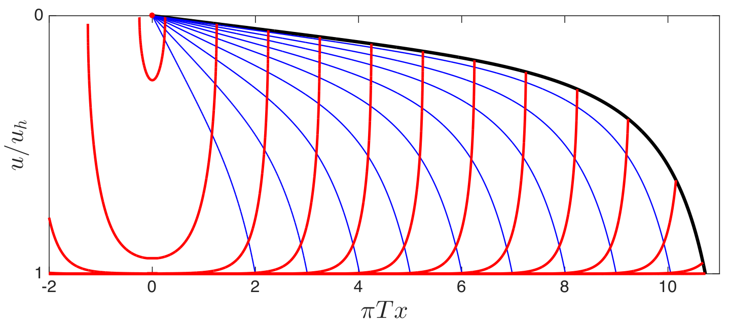
In Fig. 5 we plot a null string generated by a congruence of geodesics with . The string profile, denoted by the red curves, is shown at several values of coordinate time . The string starts off at a point on the boundary and expands at the speed of light while falling towards the horizon. The blue curves represent the null geodesics followed by bits of the string and the black curve is the endpoint trajectory. Every geodesic that makes up the string eventually falls into the horizon at some . Clearly, geodesics with smaller angle go farther, with the endpoint geodesic going the farthest and reaching the horizon after traveling a distance . Indeed, by setting , or equivalently , and expanding (43) about , we obtain the stopping distance
| (45) |
The leading order result for the thermalization distance is then given simply by
| (46) |
a result obtained previously in Ref. [30], and can be made arbitrarily large by taking the angle . We therefore see that the limit is synonymous with the limit. In what follows we shall use these two limits interchangeably.
If we denote the value of that labels a geodesic that travels a total distance before plunging into the horizon by , from (45) and (46) we then see that
| (47) |
Recall that we can isolate the SSR of Eq. (1) by taking the limit, which is to say the limit, while keeping fixed at any value between 0 and 1. Noting that above-horizon geodesics are those with , we see from (47) that in this limit, all above-horizon geodesics have .
What is the above-horizon shape of the string shown in Fig. 5? The solution to the geodesic equation (43) can also be written
| (48) |
where satisfies
| (49) |
Consider the limit of (49). When we have and the solution to (49) can be expressed in terms of hypergeometric functions. When we can approximate and , so the solution to (49) reads
| (50) |
which is simply the trailing string profile of Refs. [9, 12]. Therefore, when the string is in the SSR, everywhere except very close to its endpoint, its profile illustrated in Fig. 5, is simply the trailing string profile, suitably truncated to reflect the falling endpoint, and translating at the speed of light.
We turn now to the first order correction defined in (36). At leading order in the bookkeeping parameter , the worldsheet energy density and flux read
| (51) |
Hence, at leading order in the string equations of motion (31) simply read , meaning . In other words, energy is transported on the congruence of geodesics which make up the null string. This is a consequence of causality: in the limit where the string expands asymptotically close to the speed of light, different points on the string are causally disconnected from each other and the energy of each bit of string must be transported along the null rays that describe how the string expands.
Because is time independent, it is only necessary to compute it at one time, which for convenience we take to be an early time when the entire string is near the AdS boundary. Near the AdS boundary, where and the geodesics are given by (40), the string equation of motion leads to the equation of motion for
| (52) |
which has the solution
| (53) |
for arbitrary functions and . Upon substituting the string solution (53) and the geodesic congruence (40) and (41) into (51), we obtain
| (54) |
We now turn to enforcing the open string boundary conditions. At first order in and near the AdS boundary, where , the open string boundary conditions (32) require
| (55) |
How does vanish as ? We see from the expression (54) for the density of energy along the string per unit that finiteness of the string energy requires with . Moreover, note that in general contains a term proportional to . Finiteness of and finiteness of the total string energy therefore require to have a near-endpoint asymptotic expansion of the form
| (56) |
In the SSR, where geodesics with make up the string, we may employ the expansion (56), keeping only the leading term. Expanding (54), we then obtain the above-horizon world sheet energy density
| (57) |
We therefore see that up to an overall constant specified by , the world sheet energy density is uniquely determined in the SSR. Simply put, the large information contained in and falls into the horizon promptly after the string is created, before the string enters the SSR.
At leading order in , the string stress tensor which sources the linearized Einstein field equations is given by
| (58) |
where
| (59) |
is just the stress for a single null particle moving on a geodesic labeled by with energy .
3.2 The evolution of the jet envelope and opening angle
We wish to solve the gravitational bulk to boundary problem in the SSR. This requires focusing on , or equivalently, when . Before proceeding with the gravitational bulk to boundary problem, let us analyze the congruence of geodesics which make up the above-horizon segment of string. As discussed above, these geodesics have with given in (47). However, in the SSR it turns out that only geodesics with parametrically close to are close to the horizon. Geodesics with not close to are close to the boundary with
| (60) |
To verify these statements we employ the rescaled variables and defined in Eq. (42) and the geodesic solution (43). From (42) and (47) we have
| (61) |
Moreover, as , Eq. (43) implies that diverges like
| (62) |
It therefore follows that and, correspondingly, until becomes parametrically close to . In particular, upon substituting (61) into (62) we see that only geodesics with have and, correspondingly, . Since the string’s energy density is simply transported along the geodesics which make up the null string, and since is greatest near the endpoint, we conclude that in the limit a parametrically large fraction of the string’s above-horizon energy is located asymptotically close to the AdS boundary.
Via the gravitational bulk to boundary problem, the near-endpoint gravitational field of the string induces a highly peaked and localized stress on the boundary. The localized stress induced by the near-endpoint segment of the string must determine the jet opening angle and energy. Since the vast majority of the string’s above-horizon energy is located asymptotically close to the AdS boundary, the scale of localization of the jet must be . It follows that in the region of space where the jet is localized, one can employ zero temperature Green functions (which can be computed analytically) to solve the linearized Einstein equations and compute the near-jet boundary stress tensor. That is, close to the AdS boundary the geometry is approximately that of AdS5 and the gravitational bulk to boundary propagators take their zero temperature form. However, the source for the linearized Einstein equations — the string stress tensor — incorporates finite temperature effects that cannot be neglected. In particular, the congruence of geodesics that make up the near-endpoint segment of the string are pulled towards the horizon by the gravitational field of the black hole and this effect accumulates as the string traverses the SSR and cannot be neglected. As we shall see below, in the boundary theory the bending and falling of geodesics towards the horizon encodes the broadening of the jet opening angle.
In characterizing the bending of a geodesic towards the horizon it is useful to define the angle
| (63) |
which is simply the angle a geodesic labeled by makes with the boundary at point . At small we have . If the geodesic were propagating in vacuum, we would have for all time. However, as the geodesic propagates through the plasma it curves downward toward the horizon, meaning that increases. Using the geodesic solution (43) and the definition (63), it can be shown that
| (64) |
with
| (65) |
where is the inverse of the function defined in (44). The expression (64) describes how increases and the geodesic curves downward as it propagates. One can show directly from the geodesic solution (43) that at , where , the geodesic has , meaning that at the point where the geodesic strikes the horizon has increased to a final value , which is to say since is small. This explains why all the blue curves in the SSR in Fig. 5 strike the horizon at the same angle. Although rapidly increases to its final value as the geodesic approaches the horizon, by differentiating (64) we see that at earlier times when the geodesic is in the near-boundary domain (60), is slowly varying with . Because of this, locally near any point we may approximate the near-boundary geodesics with their tangent lines
| (66) |
where , and all depend on and . In other words, locally the geodesics take their zero temperature form (40) with accumulative finite temperature effects encoded in and and .
A consequence of the above analysis is that the near-boundary segment of string, where nearly all the above-horizon string energy is located, is just a sum of null point particles moving on trajectories which locally take the zero temperature form (66) and which have energy As we noted above, in this near-boundary region it is appropriate to use the zero temperature gravitational bulk to boundary propagators. The boundary stress tensor induced by a single null particle of energy falling in the zero temperature AdS5 geometry along a geodesic (66) was computed in Ref. [39]. Their result reads
| (67) |
where , , , and . By linearity, the full expression for the stress induced by the near-endpoint segment of the string reads
| (68) |
The integrated flux through a surface of constant , Eq. (13), therefore reads
| (69) |
As we shall see below, in the limit has a parametrically high amplitude with a parametrically small width . This justifies neglecting all other contributions to the flux except those coming from the near-endpoint segment of the string.
To proceed further it is useful to expand (69) in powers of . To do so we assume so and that . At small and in the near-boundary region (60), where , we may approximate (64) as
| (70) |
Likewise, in the small limit we may use (61) to approximate
| (71) |
Turning next to and , it follows from the geodesic equation (39) that in the near-boundary region (60). This means . Likewise, it follows from the solution (43) to the geodesic equation that in the small limit we have
| (72) |
Upon substituting Eqs. (70) and (72) and the world sheet energy density (57) into (69) and expanding in powers of , we secure the leading order result
| (73) |
again with given by (71).
Before proceeding further, several comments are in order:
- 1.
We see from (47) and (71) that the integral in (73) only depends on via the ratio . This means that upon making the rescalings and and keeping fixed, the integral in (73) is given by multiplying an expression that has a finite limit. Hence, as advertised above, as we find that has a peak value at that grows like and has a parametrically small width in that scales like .
- 2.
The integrand in (73) vanishes as where, according to Eqs. (61) and (62), grows unboundedly large. More precisely, the integrand at is suppressed in value since at the horizon and we took the limit to derive (73). This means that contributions to from the near-horizon segment of the string are suppressed in the limit relative to those from the near-endpoint segment of the string.

Figure 6: The color at a point in this plot depicts , the integrated flux of energy in the -direction that passes through a point on the planar surface at a given value of that is a given transverse distance from the center of the jet. At each value of , we normalize relative to its maximum value at that , namely . We have normalized by a factor of in order to obtain a figure that is unchanging as the limit is taken. This figure should be compared to the cartoon in Fig. 3. We shall take as our quantitative definition of the yellow region in that cartoon the region of the present figure in which is more than half its maximum value ; we could equally well have chosen a definition in which “half” was replaced, for example, by 10%. - 3.
- 4.
As , when the string endpoint falls towards the horizon and we exit the SSR, the approximations used to derive (73) and obtain Fig. 6 all break down. For example, when , the near-endpoint geodesics curve downwards rapidly and are not well approximated by the tangents (66). Furthermore, as the string endpoint falls closer and closer to the horizon, the gravitational bulk to boundary problem cannot be solved using zero temperature Green functions. For any fixed small value of , meaning for any fixed large value of , (73) and Fig. 6 are only good approximations as long as . In the limit, and the regime where they break down shrinks as a fraction of , and Fig. 6 is obtained in its entirety.
- 5.
In describing how the shape of the jet evolves as it propagates, we have focused entirely on its expansion in the directions, transverse to its direction of motion , as this transverse expansion defines the opening angle of the jet. That is, we have focused on the expansion of the vertical dimension of the red oval in the cartoons in Figs. 2 and 3. In our calculation, where we have worked to leading order in the limit, the red oval has zero longitudinal thickness. This can be seen by substituting the small limits for and given in (72) into the expressions (67) and (68) for the near-jet stress-energy. The delta function in (67) becomes which means that the longitudinal profile of the energy density depicted in the cartoons in Figs. 2 and 3 is a delta function. Of course, (72) is only valid in the SSR and to leading order in the limit. We leave the calculation of the higher order corrections which smear out the delta function to future work.
With in hand, we can now follow the prescription set out in Section 2 to define the opening angle of the jet and follow its evolution as the jet propagates through the strongly coupled plasma. In the left panel of Fig. 7, we plot the transverse envelope function , defined in Eq. (14) as the half width at half maximum of .22 2 With the explicit result (73) for available to us, we can now see why in Section 2 we chose to define the opening angle of the jet via rather than via a moment of , say . Explicit evaluation shows that the leading order contribution to in the limit, i.e. in the small opening angle limit, is divergent. The divergence reflects the fact that falls off so slowly at large that is parametrically larger than . In fact, as and the jet opening angle defined from the half width at half maximum scales to zero proportionally, the moment instead stays nonzero. As in Fig. 6, in making the plot we have normalized by a factor of so that we can plot a quantity that is fixed in the limit. The envelope function plotted in Fig. 7 is of course a constant-color contour of Fig. 6. At first grows linearly in with rate
| (74) |
However, by the rate of growth of has begun to increase. Since diverges as à la Eqs. (61) and (62), it follows that as as long as the jet is within the SSR we must have the divergence
| (75) |
However, when and the jet leaves the SSR, we see from (75) that the transverse size of the jet has grown to .
In the right panel of Fig. 7 we plot . As is evident from the figure, the transverse envelope of the jet can be approximated by33 3 Note that if we had chosen to define as the half width at 10% of maximum of instead of the half width at half maximum, which is to say if we had chosen a constant-color contour of Fig. 6 in the deep-blue rather than in the mid-green, we would have obtained in (74) and would have concluded here that to within 2.5% accuracy.
| (76) |
to within 1.5% accuracy. In other words, up to an normalization factor whose value depends on an arbitrary choice of the definition of the width of the jet, the radial coordinate of the string endpoint gives the transverse width of the jet. Indeed, using the small limit of (42) we see that the integrand in (73) is
| (77) |
The width of the integrand is just weighted by the world sheet energy (57), which diverges at the string endpoint. Therefore, it is natural that is approximately proportional to .
In the small angle limit, the opening angle of the jet that we defined in Eq. (12) is given by
| (78) |
In the left panel of Fig. 8 we plot as a function of . From (74) it follows that at small the opening angle is almost constant, hardly changing from its initial value
| (79) |
Upon solving for and plugging this result into the expression (46) for the thermalization distance, we obtain Eq. (4) in the Introduction, namely
| (80) |
with
| (81) |
We now see that the total distance that a jet can travel through plasma before thermalizing is entirely determined by the temperature and the initial opening angle alone. The initial energy of the jet need not be known, although as we shall see in Section 3.3 it must be greater than some minimal value that depends on the initial opening angle.
Mirroring the behavior of , after initially increasing only very slowly, by the rate of growth of has begun to increase. As increases further, as long as the jet is in the SSR we can see from (78), (75) and (80) that increases like
| (82) |
When , the jet exits the SSR, our analysis breaks down, and the jet is no longer crisply defined. This occurs when has increased to the point that . We therefore conclude that the jet thermalizes when its opening angle is of order 1 and its transverse size is of order .
In the right panel of Fig. 8 we plot the jet angle normalized by . Again, we see that
| (83) |
to within 1.5% accuracy. This simply follows from (76) and the small angle limit of the definition of in (63). Via Eqs. (70), (71), and (47), we therefore obtain
| (84) |
stated in the Introduction in Eq. (5). The expansion (7) is then obtained by expanding this result in powers of . Equivalently, we can start by expanding the RHS of (43) in powers of , since is small when is small, obtaining
| (85) |
then invert this series obtaining the small expansion of , and then substitute the resulting series into (70) and expand again, obtaining the small expansion of which, using (42), takes the form
| (86) |
Using (83) and (46) and defining as in (8), we obtain (7), as stated in the Introduction.
We close this Section by comparing the exact result for , given in (64), to the small-angle approximation of given (70). This comparison is useful because it gives one an estimate of the domain of utility of our approximations for finite . How big is the SSR for some given ? In Fig. 9 we show the comparison between Eqs. (64) and (70) at various values of . We see from the figure that the small angle approximation works very well where is almost constant and for the portion of its upward rise up until . The range of where the colored curve peels away from its dashed approximation therefore corresponds to the range of where the string leaves the SSR and our analysis of the energy loss rate and opening angle evolution breaks down. Simply put, beyond this point, the instantaneous energy loss rate and opening angle are not crisply defined as the jet blurs as it thermalizes.
3.3 Rate of energy loss
We now perform the holographic computation of the rate at which the jet loses energy to hydrodynamic modes of the plasma, which is to say the rate at which energy flows through the yellow sphere in Fig. 2. As we discussed in Section 2, in order to compute the rate of energy loss of the jet in the boundary gauge theory , we need the transverse traceless mode of the stress tensor of the boundary gauge theory. From the relationship between the SYM stress and the metric perturbation , Eq. (29), it is clear that the transverse traceless mode of the SYM stress is encoded in the transverse traceless mode of , which in turn is sourced by the string stress tensor that we obtained in Eq. (58). We now develop these relationships explicitly.
Let
| (87) |
be the Fourier transform of and define the transverse traceless gravitational mode
| (88) |
It is then straightforward to show from the linearized Einstein field equations (27) that obeys the ordinary differential equation [16]
| (89) |
where and
| (90) |
with the Fourier transform of the string stress tensor and . With the boundary condition , the ODE (89) implies that has the near-boundary asymptotic behavior
| (91) |
with
| (92) |
From the definition of the transverse traceless mode of the SYM stress in Eq. (23), and the relationship between and in Eq. (29), we therefore conclude that the transverse traceless mode of the boundary gauge theory stress tensor, defined in (23), is given by
| (93) |
Therefore, computing the long wavelength limit of is tantamount to solving (89) in the long wavelength limit.
To solve (89) we construct a Green’s function out of homogeneous solutions and ,
| (94) |
where is the Wronskian of and . The appropriate homogeneous solutions are dictated by boundary conditions. The differential operator in (89) has singular points at and . At the indicial exponents are and while at they are . Vanishing of at the boundary requires as , while the requirement that the black hole not radiate requires as . We choose normalization so that . With this choice, the coefficient reads
| (95) |
The integrand has two pieces, one coming from the homogeneous solutions and one coming from the string stress tensor. We take them in turn.
In the long wavelength limit , the homogeneous solutions to Eq. (89) can be computed analytically and read and We therefore secure the long wavelength asymptotic behavior
| (96) |
that is the first ingredient needed in order to evaluate (95) and hence (89) at long wavelengths.
Next, we need . We choose polarization vectors
| (97) |
with and . Fourier transforming the string stress (58), we obtain
| (98) |
where is given by the solution to and is given by Eq. (43). Using Eqs. (98), (97) and (90), the source reads
| (99a) | ||||
| (99b) | ||||
We now have all the pieces needed to evaluate (95). Using the long wavelength solution (96) and the source (99), we conclude from (95) that the long wavelength limit of the coefficient is given by
| (100a) | ||||
| (100b) | ||||
We wish to evaluate the radial integral in (100a) in the limit with and fixed. The integral is dominated by . In the region the geodesic equations (39) imply . Furthermore, we see from the geodesic equations (39) that . This means the radial integrand in (100a) reads
| (101) |
Therefore, in the IR the radial integral in (100a) evaluates to
| (102) |
where we have used .
Using (102), (100a) and (93), we therefore conclude that the long wavelength limit of the transverse traceless mode of the gauge theory stress tensor reads
| (103) |
We have achieved our goal; what remains is interpreting (103) and understanding its consequences.
Eq. (103), should be compared to the expected form in Eq. (24). Substituting both and the polarization vectors (97) into (24), and comparing to (103), we see that the jet energy must be given by
| (104) |
Fourier transforming back to real space, the leading order derivative expansion of the jet energy reads
| (105) |
The first term in (105) just corresponds to the energy added when the jet is created while the second encodes the energy loss of the jet while it propagates through the plasma. Using the fact that the jet moves at nearly the speed of light, the energy lost per unit distance traveled reads
| (106) |
where is given in (47). In the dual gravitational picture, the energy loss rate (106) is nothing more than the rate at which the string’s energy flows into the horizon. This was introduced as a definition in Ref. [30]. We now see that this is indeed the natural definition, as it is equivalent to defining the energy loss rate in the field theory as the rate at which energy flows into hydrodynamic modes, which is to say the rate at which energy flows through the yellow sphere in Fig. 2.
Using Eqs. (57), (47) and (46), it is a straightforward exercise to show that (106) yields
| (107) |
our result for the rate of energy loss, given in the Introduction as Eq. (10), discussed there extensively, and derived previously in Ref. [30], with the initial energy given by
| (108) |
As in our calculation of the evolution of the opening angle of the jet in Section 3.2, these expressions are valid only in the SSR. In the limit, the SSR extends to arbitrarily close to 1, meaning that (107) can be used until is arbitrarily close to 0. For jets with a large but finite , meaning a small but nonzero initial opening angle, (107) breaks down where and the jet leaves the SSR. is the energy of the jet when it enters the SSR. It is impossible to define the jet energy from the distribution of energy along the string before the string enters the SSR because at the moment of its creation the string describes gluon fields around its creation event as well as the jet, and we need to wait for the jet to separate from extraneous, transient, gluonic excitations which are not comoving with the jet and which therefore fall into the horizon within a time of order before defining . In the limit, the jet enters the SSR at a value of that is arbitrarily close to 0, and the result (107) can be applied for and describes the evolution of from to 0.
Upon solving (108) for and substituting into (46) and (79), we obtain the relationship between the initial energy and both the thermalization distance and the initial opening angle:
| (109) |
both results that we gave in the Introduction, namely Eqs. (3) and (2), now with an explicit expression for the energy scale :
| (110) |
The preparation of the initial state of the string enters , and hence our results (2) and (3), only through the constant defined in (56). We see from (2) and (110) that is fully specified by and . Through (4) we see that and specify meaning that (through (10) or (11) and (5) or (7)) , and fully specify the rate of energy loss and the evolution of the jet opening angle as the jet propagates through the plasma.
What is the gravitational origin of the divergence in as that is apparent in (107)? The opening string boundary conditions require that the string endpoint moves at the speed of light. This in turn means that must diverge at the endpoint, as Eq. (57) demonstrates, since the string has finite tension. As , the flux of energy into the horizon must increase because more and more of the near-endpoint geodesics fall into the horizon. Simply put, the dramatic increase in the energy loss rate as encodes the fact that the string endpoint energy density is divergent and the last to fall into the horizon.
The relationship between the initial opening angle and the initial energy of the jet depends on the details of how the state is prepared, details that are encoded in the value of . We can now see why must have a minimum value. From (110) we see that decreasing corresponds to increasing . However, this cannot be done without bound, since the geometric optics expansion (35) will eventually break down. Equating derivatives of the zeroth and first order terms in the geometric expansion, , via Eqs. (42), (43), (51) and (57) we estimate that the geometric optics expansion breaks down when , which means . Equivalently, this means that the dimensionless constant introduced in the Introduction via has a maximum value which is of order 1. Indeed, both analytical arguments and numerical solutions to the string equation of motion suggest that the maximum value of ranges between 0.5 and 1 [19, 27]. The fact that has a minimum possible value corresponds to the statement that jets with a given can have any initial energy above some minimum possible value, or to the statement that jets with a given must have initial opening angles greater than some minimum possible value. Knowing the initial energy of a jet requires knowing both its initial opening angle and the details of how it was prepared that are encoded in and hence . Therefore, the relationship between the initial energy of the jet and its thermalization distance also depends on these details. But, the relationship between the initial opening angle of the jet and its thermalization distance is independent of any details concerning how the state is prepared; it is fully specified by (4). This is one of the central lessons we learn from our calculation.
While we have obtained the energy loss rate from the rate that energy flows into IR modes, we note that we could have equally well obtained the energy loss rate from the rate that energy leaves UV modes. Specifically, it must be that
| (111) |
with given in (68). Indeed, a straightforward calculation shows this to be the case.
4 Qualitative lessons for jets in heavy ion collisions
We have provided a complete summary of all of our central results, in their own context, in the Introduction. That is, we described the conclusions that we draw from our results and their many consequences and implications for the behavior of the jets in SYM theory that we have analyzed. We shall not repeat these conclusions and observations here. Our purpose in this Section is to speculate as to how one may draw qualitative lessons for jets in QCD, as produced and subsequently quenched in heavy ion conclusions, from our results.
As we already noted in Section 1, there are two broad paths possible here. The more conservative approach is to observe that perturbative QCD does a fine job of describing the high-momentum-transfer physics of jet production and jet fragmentation, and conclude that we should use insights gleaned from calculations in strongly coupled SYM theory only to guide how we treat the low-momentum-transfer interactions between the individual partons within a QCD jet shower and the strongly coupled quark-gluon plasma in which they find themselves. The first steps down this path have been taken in Refs. [31, 33], with the construction of a hybrid model that utilizes the form of the expressions (10) and (3) that we have rederived for the rate of energy loss of SYM jets to describe the rate of energy loss of partons in a shower that is otherwise as described by perturbative QCD. Our work supports this approach via rederiving (10) and (3) without assuming a slab of plasma and with defined entirely within the gauge theory. It is interesting to ask how our results concerning the opening angle of the SYM theory jets that we have analyzed can inform future extensions of the hybrid model of Refs. [31, 33]. Its simplest incarnation which has been used to this point relies upon (3) with a single, in effect average, value of that has been obtained for jets in quark-gluon plasma via a fit to heavy ion collision data. From (2) we now see that for a given the constant is different for jets with different initial opening angles. So, possible extensions to the hybrid model could either introduce a probability distribution for reflecting the distribution of initial opening angles or could directly relate to the initial energy and initial opening angle of each jet in a Monte Carlo sample according to (2), in effect introducing an initial-opening-angle-dependent rather than fitting a single average value in units of . After extending the model in this way one could then use (4) to fix for each jet after which the energy lost by each parton in that jet could be described by (10) as in Refs. [31, 33]. In implementing this procedure, the value of the constant in (2) and (4) could be allowed to float, fitting it to data in order to incorporate the differences between quark-gluon plasma and SYM plasma. Another possible extension would be to somehow encode our result (7) for how the opening angle of the SYM jets increases as they propagate in a probability distribution for the transverse kicks that the partons in a perturbative QCD shower receive as they propagate through strongly coupled quark-gluon plasma, adding the effects of such kicks to the hybrid model of Refs. [31, 33].
The more ambitious approach is to try to use insights gleaned from our results for SYM jets to obtain qualitative insights into the behavior of QCD jets in their entirety, without relying on a perturbative QCD parton-by-parton description of the jets at all. In the remainder of this Section, we look toward a variety of possible comparisons between the behavior of SYM jets and the behavior of jets in heavy ion collisions, as described perturbatively or as measured in experiments:
- •
It is interesting that, as we explain in full in Appendix A, we find that the ratio of the initial jet mass to the initial jet energy is not a good proxy for the jet opening angle , because it is sensitive to the contribution of the “tails” of the jets at angles that are substantially greater than . This supports the use of measures of the jet opening angle that, like the half width at half maximum definition of that we have employed, are defined from the jet shape, a quantity which has been measured in heavy ion collisions [40]. Via suitable modelling in a Monte Carlo study, it may also be possible to relate such measures to the ratios of the inclusive cross-sections for the production of jets reconstructed from experimental data using different values of the radius parameter in the anti- reconstruction algorithm as in Refs. [41, 42].
- •
Perhaps our most interesting result is the relationship (4) between and . Together with (10), this tells us that jets with a smaller (larger) initial opening angle lose less (more) energy. At a qualitative level, this is also certainly the case for jets in perturbative QCD, for the simple reason that in perturbative QCD a jet with a larger initial opening angle is a jet that has fragmented into more partons and in particular into more resolved subjet structures, each of which loses energy as it passes through the plasma, meaning that a large-angle jet loses more energy in sum than a narrow jet containing fewer partons does [43]. It is in fact very important to keep this feature in mind in analyzing jet data. If we compare two samples of jets in heavy ion collisions that have, on average, lost different amounts of energy — for example a sample of leading jets (those that are the most energetic jets in their event) and a sample of jets that are the lower-energy jets in a dijet pair — then the leading jets will on average be those which had a smaller initial opening angle. The importance of this effect has recently been emphasized [44, 33]. (The leading jets will also on average be those which have travelled through a shorter length of plasma, but Monte Carlo studies suggest that this may be the less important effect [44].)
- •
Although narrow jets lose less energy than wide jets both in SYM theory and in perturbative QCD, there can certainly be qualitative differences. For example, it is striking that, as we discussed in Section 1 via our results (4) and (10), the initial opening angle of the SYM jets controls their fractional energy loss . It would be interesting to investigate whether this qualitative regularity applies also to jets in perturbative QCD, but this is not expected since in perturbative calculations of parton energy loss one obtains a for each parton (more precisely, each resolved subjet) that is independent of its initial energy or depends on it only logarithmically [45, 46, 47, 48, 49].
- •
Our results make it clear that it would be exceedingly interesting to tag jets in heavy ion collisions according to what their opening angle would have been if they were produced in vacuum. Unfortunately, we know of no way to do this. One can to some degree tag jets by what their energy would have been if they were produced in vacuum by looking at jets produced back-to-back with a photon or Z-boson whose energy is measured. But, we do not know of any way to know what the opening angle of a particular jet seen in a heavy ion collision would have been if it had not interacted with any quark-gluon plasma, i.e. if it had instead been produced in an elementary collision in vacuum. This makes it particularly important to attempt a comparison between the qualitative features of the relationship between and energy loss in (4) and (10) to that same relationship in Monte Carlo implementations of jet quenching in perturbative QCD, like for example JEWEL [44, 50].
- •
In any future comparison between (4) and (10) on the one hand and information about the relationship between jet angle and jet energy loss in QCD, either from Monte Carlo studies or from experiment, it will be important to treat the purely numerical prefactor in (4) as a free parameter. If the relationship (4) turns out to be a good description of the behavior of jets in QCD, the value of the purely numerical prefactor must be different in QCD than in SYM theory because the plasmas of the two theories have different degrees of freedom.
- •
The difficulty in identifying what the opening angle of a particular jet seen in a heavy ion collision would have been in vacuum makes it hard to compare the most striking qualitative features of our results to experimental data in a direct fashion. It should nevertheless be possible to make such a comparison, albeit slightly more indirectly. One path to a comparison with experimental data is to (i) create an ensemble of SYM jets with varying and , perhaps choosing the distribution of for jets with a given following results from perturbative QCD; (ii) then define for each of the jets in the ensemble from according to (4), treating as a free parameter to be varied; and (iii) then send this ensemble of jets through a length of plasma that is small compared to all of their ’s. With this setup, the decrease in the energy of each jet can be obtained from (11) and the increase in the opening angle of each jet can be obtained from (7). Because the expansion (7) starts at a higher power of than the expansion (11), we expect that in a regime in which the fractional energy loss is small the growth in the jet opening angle will be even smaller. Nevertheless, because the probability distribution for is steeply falling and that for is nontrivial, the effects of passing the ensemble of jets through the plasma on these distributions could be nontrivial. It would be very interesting to see how the final double-distribution, as a function of and , compares to the initial double-distribution, to ask under what circumstances the final distribution looks like a scaled version of the initial distribution, and to compare (suitable integrals of) the final double-distribution to data.
- •
Although perhaps less relevant to data, since what experimentalists typically see are jets that emerge from a heavy ion collision as jets not jets that have thermalized, it is also interesting to look at the qualitative behavior of SYM jets as they thermalize. They lose a large fraction of their energy over the last small fraction of their lifetime, reminiscent of a Bragg peak [19, 30]. And, at the end of their lifetime as they thermalize their opening angle grows rapidly, until it is of order 1, and their transverse size also grows rapidly, until it is of order . The question of whether analogous behavior is seen in jets in perturbative QCD could be investigated in Monte Carlo studies. Although challenging, it may also be possible to investigate such behavior via measuring jets as correlated energy flow over regions of large jet radius in events selected by triggering on a photon or Z boson.
At present it is too soon to tell how the many interesting qualitative features of our results for the behavior of the energy and opening angle of SYM jets compare to experimental data or to calculations based upon perturbative QCD. Such comparisons will ultimately determine how valuable it is to compare SYM jets to QCD jets, which is to say how many qualitative lessons from the former apply to the latter. Even if such comparisons remain as challenging as they are at present or turn out unsuccessfully, though, the use of our results in (future generalizations of) the hybrid strong/weak coupling model of Refs. [31, 33] will remain important, given how successfully the simplest one-parameter version of this model has been able to describe so much jet data to date.
Note Added:
Since v1 of this paper was posted, in Ref. [51] Milhano and Zapp have completed the work that we have cited as a private communication [44]. They conclude from their analysis using the JEWEL event generator [50] that the dijet asymmetry seen in LHC heavy ion collisions depends largely on the asymmetry between the initial opening angles of the two jets and only to a subleading degree on the asymmetry between the lengths of plasma which the two jets traverse. As they note, their results — obtained in a calculation done entirely upon assuming weak coupling — are in qualitative agreement with our result — obtained in a calculation done entirely upon assuming strong coupling — that the fractional jet energy loss is controlled by the initial jet opening angle.
Also since v1 of this paper was posted, in Ref. [52] Casalderrey-Solana and Ficnar have presented beautiful results from a holographic calculation of three-jet events in strongly coupled SYM plasma. They analyze classical string configurations with non-trivial transverse dynamics in the initial state. They find that their initial wave on the string develops into a kink-like structure which can correspond in the gauge theory to a three-jet event, with the string endpoints corresponding to quark jets and the kink corresponding to a gluon jet. Their study is the first analysis of proxies for three-jet events in a holographic context. One of their central results can be described in terms of results that we have obtained by observing that their quark and gluon jets propagate through the plasma as two separate jets if and only if the angular separation between them is greater than the initial opening angle of each jet separately. They find that if their angular separation is less than this, the string endpoint and the kink in the gravitational theory describe a single jet with substructure, not two jets. In particular, Casalderrey-Solana and Ficnar focus on identifying the smallest possible angular separation between two resolved jets for a quark jet and a gluon jet with a particular summed energy. Since resolving the two jets requires them to be separated by more than their individual initial opening angles, minimizing their separation means minimizing their individual opening angles in (2). This means that the jets must be prepared with the minimum possible value of or, equivalently from (110), the maximum possible value of . Noting that the minimum possible value of is proportional to , the parametric dependence of in (2) reproduces the parametric dependence of the smallest possible angular separation between two resolved jets identified in the calculations reported in Ref. [52].
Acknowledgements.
We acknowledge helpful discussions with Jorge Casalderrey-Solana, Doga Gulhan, Peter Jacobs, Kristan Jensen, Yen-Jie Lee, Guilherme Milhano, Daniel Pablos, Andrey Sadofyev, Konrad Tywoniuk, Wilke van der Schee and Korinna Zapp, and in particular thank Guilherme Milhano and Korinna Zapp for a discussion of their work in progress. KR is grateful to the CERN Theory Division for hospitality as this research was being done. The work of PC was supported by the Fundamental Laws Initiative at Harvard. The work of KR was supported by the U.S. Department of Energy under Contract Number DE-SC0011090.Appendix A The jet mass
We define the initial jet mass via the initial energy and momentum of the jet:
| (112) |
where the jet energy and momentum are
| (113) |
where both integrals are to be evaluated at a time that is and . Writing and assuming , the jet mass reads
| (114) |
How does the initial jet mass scale with the opening angle in the limit ? From (79) we see that this question is equivalent to asking how the initial jet mass scales with the angle in the limit. To this end, let us now express (114) in terms of the dual string variables. From the zero temperature results for the stress in Eqs. (67) and (68) and the definitions of the jet energy and momentum in (113), it is easy to see that
| (115) |
from which we can write
| (116) |
where in the last line we have used (41).
From (116) and the near-endpoint behavior of in (57), we see that is finite in the limit. In contrast, the initial jet energy in (108) diverges like . We therefore conclude , or equivalently from (79),
| (117) |
a result that we quoted in Eq. (21).
The origin of the peculiar scaling (117) is that there is energy flowing at large angles, or more precisely at angles that are large compared to in the limit, and although this energy is not significant enough to have much of an affect on as we have defined it via , the half width at half maximum of illustrated in Figs. 6 and 7, it does increase sufficiently to yield the scaling (117). This is the reason why throughout this paper we have used the definition of the opening angle that we have used, a definition that is analogous to defining it from the half width at half maximum of the jet shape, rather than attempting to define an opening angle via the jet mass. Of course, using a definition based upon, say, the half width at 10% maximum of would be just as good. But, as we noted in Section 3.2, moments of like for example are controlled by the large- tails of the distribution , and so cannot be used.
References
- [1] J. M. Maldacena, The Large N limit of superconformal field theories and supergravity, Int. J. Theor. Phys. 38 (1999) 1113–1133, [hep-th/9711200]. [Adv. Theor. Math. Phys.2,231(1998)].
- [2] E. Witten, Anti-de Sitter space and holography, Adv. Theor. Math. Phys. 2 (1998) 253–291, [hep-th/9802150].
- [3] S. S. Gubser, I. R. Klebanov, and A. M. Polyakov, Gauge theory correlators from noncritical string theory, Phys. Lett. B428 (1998) 105–114, [hep-th/9802109].
- [4] S. S. Gubser and A. Karch, From gauge-string duality to strong interactions: A Pedestrian’s Guide, Ann. Rev. Nucl. Part. Sci. 59 (2009) 145–168, [arXiv:0901.0935].
- [5] J. Casalderrey-Solana, H. Liu, D. Mateos, K. Rajagopal, and U. A. Wiedemann, Gauge/String Duality, Hot QCD and Heavy Ion Collisions, Cambridge University Press, 2014; also, arXiv:1101.0618.
- [6] M. Chernicoff, J. A. Garcia, A. Guijosa, and J. F. Pedraza, Holographic Lessons for Quark Dynamics, J. Phys. G39 (2012) 054002, [arXiv:1111.0872].
- [7] O. DeWolfe, S. S. Gubser, C. Rosen, and D. Teaney, Heavy ions and string theory, Prog.Part.Nucl.Phys. 75 (2014) 86–132, [arXiv:1304.7794].
- [8] P. M. Chesler and W. van der Schee, Early thermalization, hydrodynamics and energy loss in AdS/CFT, Int. J. Mod. Phys. E24 (2015) 1530011, [arXiv:1501.0495].
- [9] C. P. Herzog, A. Karch, P. Kovtun, C. Kozcaz, and L. G. Yaffe, Energy loss of a heavy quark moving through N=4 supersymmetric Yang-Mills plasma, JHEP 07 (2006) 013, [hep-th/0605158].
- [10] J. Casalderrey-Solana and D. Teaney, Heavy quark diffusion in strongly coupled N=4 Yang-Mills, Phys. Rev. D74 (2006) 085012, [hep-ph/0605199].
- [11] H. Liu, K. Rajagopal, and U. A. Wiedemann, Calculating the jet quenching parameter from AdS/CFT, Phys. Rev. Lett. 97 (2006) 182301, [hep-ph/0605178].
- [12] S. S. Gubser, Drag force in AdS/CFT, Phys. Rev. D74 (2006) 126005, [hep-th/0605182].
- [13] M. Chernicoff, J. A. Garcia, and A. Guijosa, The Energy of a Moving Quark-Antiquark Pair in an N=4 SYM Plasma, JHEP 09 (2006) 068, [hep-th/0607089].
- [14] P. M. Chesler and L. G. Yaffe, The Wake of a quark moving through a strongly-coupled plasma, Phys. Rev. Lett. 99 (2007) 152001, [arXiv:0706.0368].
- [15] S. S. Gubser, S. S. Pufu, and A. Yarom, Sonic booms and diffusion wakes generated by a heavy quark in thermal AdS/CFT, Phys. Rev. Lett. 100 (2008) 012301, [arXiv:0706.4307].
- [16] P. M. Chesler and L. G. Yaffe, The Stress-energy tensor of a quark moving through a strongly-coupled N=4 supersymmetric Yang-Mills plasma: Comparing hydrodynamics and AdS/CFT, Phys. Rev. D78 (2008) 045013, [arXiv:0712.0050].
- [17] S. S. Gubser, D. R. Gulotta, S. S. Pufu, and F. D. Rocha, Gluon energy loss in the gauge-string duality, JHEP 10 (2008) 052, [arXiv:0803.1470].
- [18] M. Chernicoff and A. Guijosa, Acceleration, Energy Loss and Screening in Strongly-Coupled Gauge Theories, JHEP 06 (2008) 005, [arXiv:0803.3070].
- [19] P. M. Chesler, K. Jensen, A. Karch, and L. G. Yaffe, Light quark energy loss in strongly-coupled N = 4 supersymmetric Yang-Mills plasma, Phys. Rev. D79 (2009) 125015, [arXiv:0810.1985].
- [20] P. Arnold and D. Vaman, Jet quenching in hot strongly coupled gauge theories revisited: 3-point correlators with gauge-gravity duality, JHEP 10 (2010) 099, [arXiv:1008.4023].
- [21] P. Arnold and D. Vaman, Jet quenching in hot strongly coupled gauge theories simplified, JHEP 04 (2011) 027, [arXiv:1101.2689].
- [22] P. Arnold and D. Vaman, Some new results for ’jet’ stopping in AdS/CFT: long version, J. Phys. G38 (2011) 124175, [arXiv:1106.1680].
- [23] P. M. Chesler, Y.-Y. Ho, and K. Rajagopal, Shining a Gluon Beam Through Quark-Gluon Plasma, Phys. Rev. D85 (2012) 126006, [arXiv:1111.1691].
- [24] A. Ficnar, AdS/CFT Energy Loss in Time-Dependent String Configurations, Phys. Rev. D86 (2012) 046010, [arXiv:1201.1780].
- [25] P. Arnold, P. Szepietowski, and D. Vaman, Coupling dependence of jet quenching in hot strongly-coupled gauge theories, JHEP 07 (2012) 024, [arXiv:1203.6658].
- [26] P. Arnold, P. Szepietowski, D. Vaman, and G. Wong, Tidal stretching of gravitons into classical strings: application to jet quenching with AdS/CFT, JHEP 02 (2013) 130, [arXiv:1212.3321].
- [27] A. Ficnar and S. S. Gubser, Finite momentum at string endpoints, Phys.Rev. D89 (2014), no. 2 026002, [arXiv:1306.6648].
- [28] A. Ficnar, S. S. Gubser, and M. Gyulassy, Shooting String Holography of Jet Quenching at RHIC and LHC, Phys. Lett. B738 (2014) 464–471, [arXiv:1311.6160].
- [29] P. M. Chesler, M. Lekaveckas, and K. Rajagopal, Heavy quark energy loss far from equilibrium in a strongly coupled collision, JHEP 1310 (2013) 013, [arXiv:1306.0564].
- [30] P. M. Chesler and K. Rajagopal, Jet quenching in strongly coupled plasma, Phys. Rev. D90 (2014), no. 2 025033, [arXiv:1402.6756].
- [31] J. Casalderrey-Solana, D. C. Gulhan, J. G. Milhano, D. Pablos, and K. Rajagopal, A Hybrid Strong/Weak Coupling Approach to Jet Quenching, JHEP 10 (2014) 19, [arXiv:1405.3864].
- [32] R. Rougemont, A. Ficnar, S. Finazzo, and J. Noronha, Energy loss, equilibration, and thermodynamics of a baryon rich strongly coupled quark-gluon plasma, arXiv:1507.0655.
- [33] J. Casalderrey-Solana, D. C. Gulhan, J. G. Milhano, D. Pablos, and K. Rajagopal, Predictions for Boson-Jet Observables and Fragmentation Function Ratios from a Hybrid Strong/Weak Coupling Model for Jet Quenching, arXiv:1508.0081.
- [34] Y. Hatta, E. Iancu, and A. H. Mueller, Jet evolution in the N=4 SYM plasma at strong coupling, JHEP 05 (2008) 037, [arXiv:0803.2481].
- [35] D. M. Hofman and J. Maldacena, Conformal collider physics: Energy and charge correlations, JHEP 05 (2008) 012, [arXiv:0803.1467].
- [36] P. M. Chesler, K. Jensen, and A. Karch, Jets in strongly-coupled N = 4 super Yang-Mills theory, Phys. Rev. D79 (2009) 025021, [arXiv:0804.3110].
- [37] A. Karch and E. Katz, Adding flavor to AdS / CFT, JHEP 06 (2002) 043, [hep-th/0205236].
- [38] S. de Haro, S. N. Solodukhin, and K. Skenderis, Holographic reconstruction of space-time and renormalization in the AdS / CFT correspondence, Commun. Math. Phys. 217 (2001) 595–622, [hep-th/0002230].
- [39] Y. Hatta, E. Iancu, A. H. Mueller, and D. N. Triantafyllopoulos, Aspects of the UV/IR correspondence : energy broadening and string fluctuations, JHEP 02 (2011) 065, [arXiv:1011.3763].
- [40] CMS Collaboration, S. Chatrchyan et al., Modification of jet shapes in PbPb collisions at TeV, Phys. Lett. B730 (2014) 243–263, [arXiv:1310.0878].
- [41] ALICE Collaboration, J. Adam et al., Measurement of jet quenching with semi-inclusive hadron-jet distributions in central Pb-Pb collisions at TeV, JHEP 09 (2015) 170, [arXiv:1506.0398].
- [42] STAR Collaboration, P. M. Jacobs and A. Schmah, Measurements of jet quenching with semi-inclusive charged jet distributions in collisions at =200 GeV, 2015. arXiv:1512.0878.
- [43] J. Casalderrey-Solana, Y. Mehtar-Tani, C. A. Salgado, and K. Tywoniuk, New picture of jet quenching dictated by color coherence, Phys. Lett. B725 (2013) 357–360, [arXiv:1210.7765].
- [44] G. Milhano and K. C. Zapp. Private communication.
- [45] R. Baier, Y. L. Dokshitzer, A. H. Mueller, S. Peigne, and D. Schiff, Radiative energy loss of high-energy quarks and gluons in a finite volume quark - gluon plasma, Nucl. Phys. B483 (1997) 291–320, [hep-ph/9607355].
- [46] R. Baier, Y. L. Dokshitzer, A. H. Mueller, S. Peigne, and D. Schiff, Radiative energy loss and p(T) broadening of high-energy partons in nuclei, Nucl. Phys. B484 (1997) 265–282, [hep-ph/9608322].
- [47] M. Gyulassy, P. Levai, and I. Vitev, NonAbelian energy loss at finite opacity, Phys. Rev. Lett. 85 (2000) 5535–5538, [nucl-th/0005032].
- [48] M. Gyulassy, P. Levai, and I. Vitev, Reaction operator approach to nonAbelian energy loss, Nucl. Phys. B594 (2001) 371–419, [nucl-th/0006010].
- [49] Y. Mehtar-Tani, J. G. Milhano, and K. Tywoniuk, Jet physics in heavy-ion collisions, Int. J. Mod. Phys. A28 (2013) 1340013, [arXiv:1302.2579].
- [50] K. C. Zapp, JEWEL 2.0.0: directions for use, Eur. Phys. J. C74 (2014), no. 2 2762, [arXiv:1311.0048].
- [51] J. G. Milhano and K. C. Zapp, Origins of the di-jet asymmetry in heavy ion collisions, arXiv:1512.0810.
- [52] J. Casalderrey-Solana and A. Ficnar, Holographic Three-Jet Events in Strongly Coupled N=4 Yang-Mills Plasma, arXiv:1512.0037.